
Analysis of Numerical Instability Factors and Geometric Reconstruction in 3D SIMP-Based Topology Optimization Towards Enhanced Manufacturability


Abstract
1. Introduction
2. Topology Optimization of the Mathematical Model Based on SIMP
2.1. Density Filter Method
2.2. Objective Function and Constraints
2.3. Method of Moving Asymptotes (MMA)
3. Analysis of the Influencing Factors in Topology Optimization
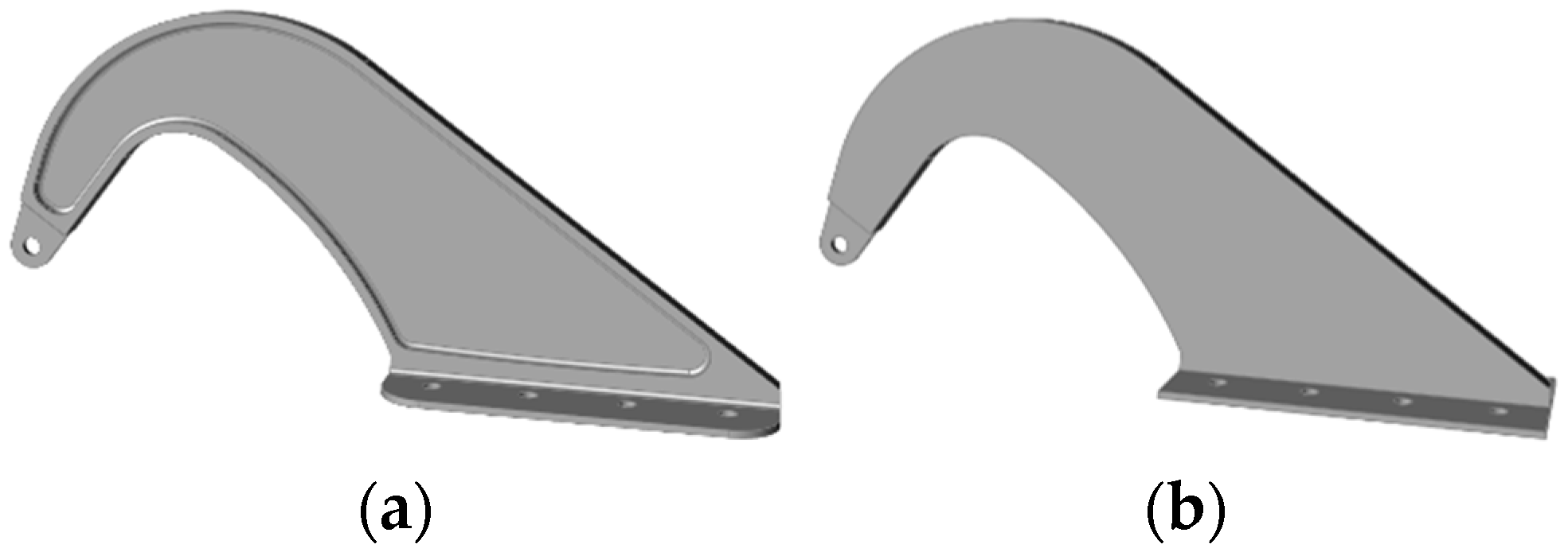
3.1. Geometric Model Simplification
3.2. Default Settings
3.3. Volume Fraction
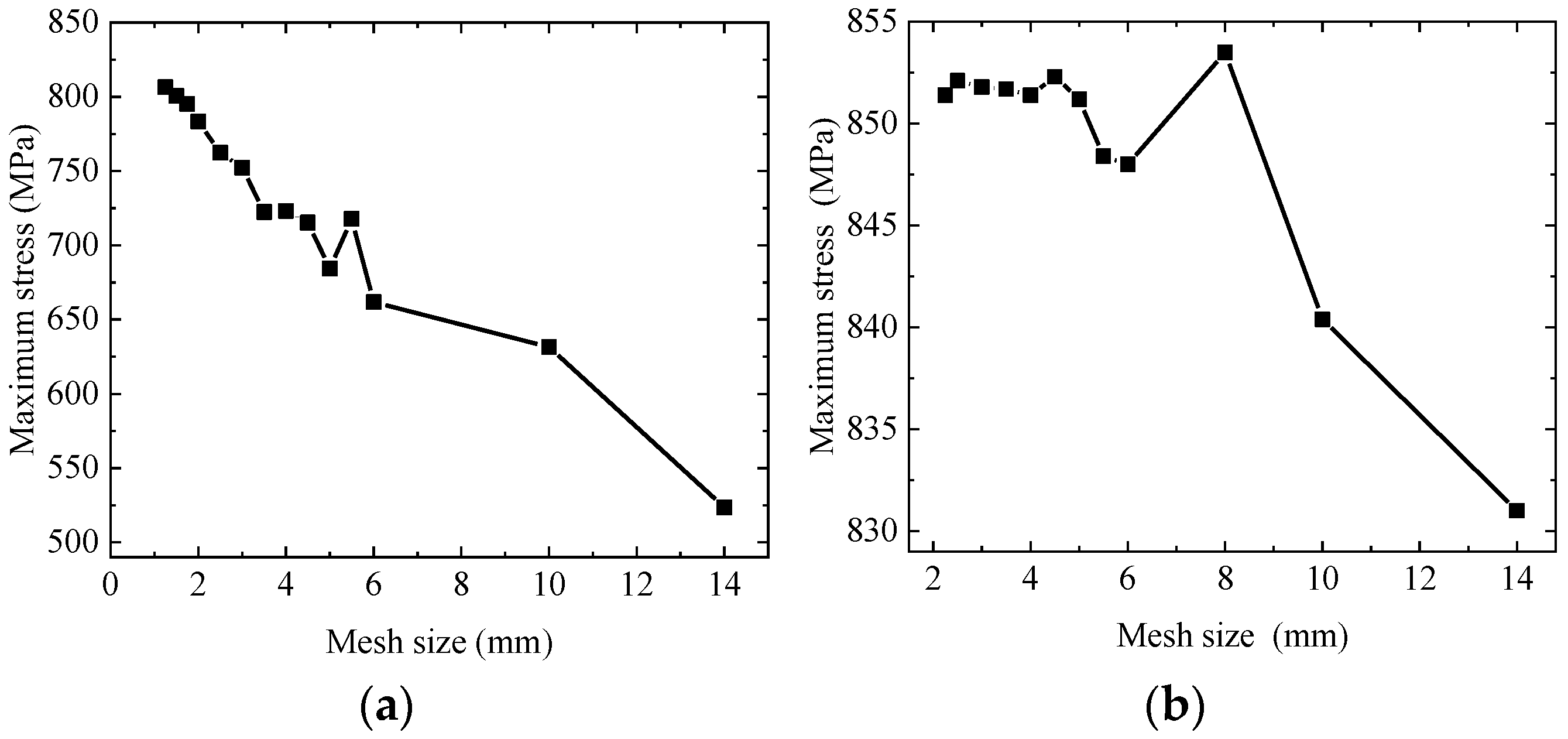
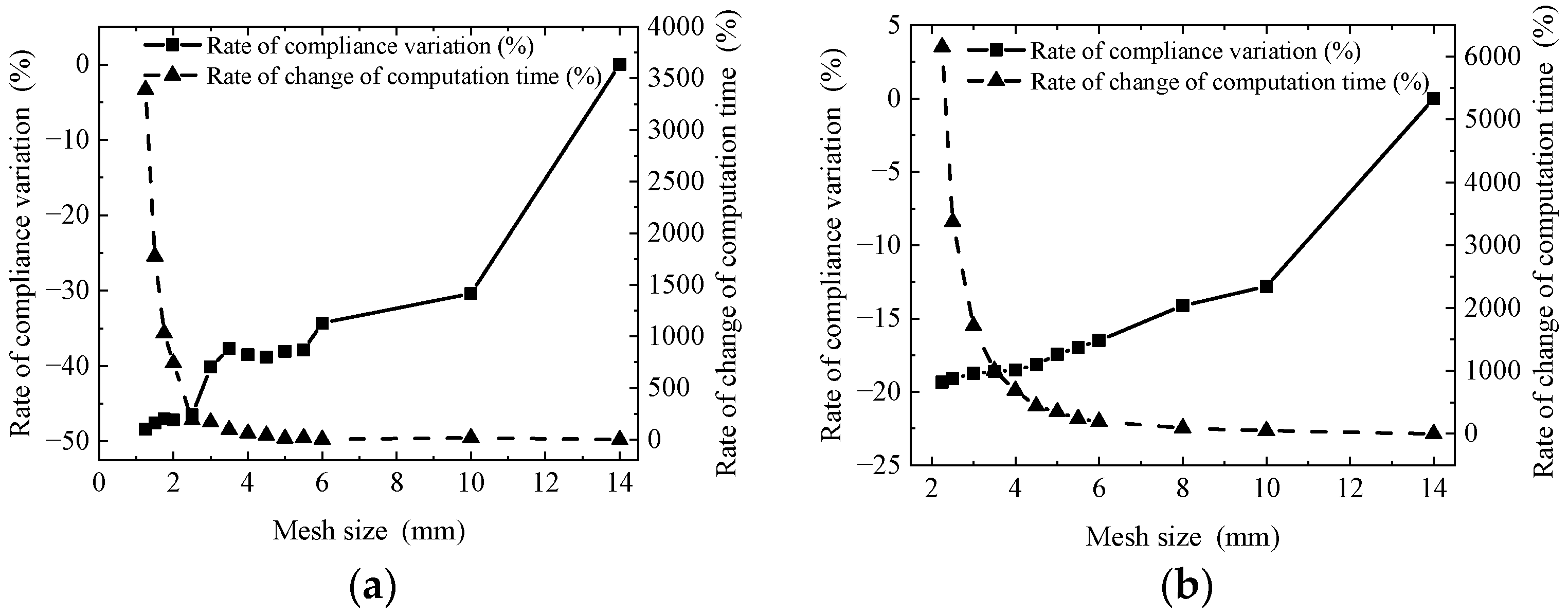
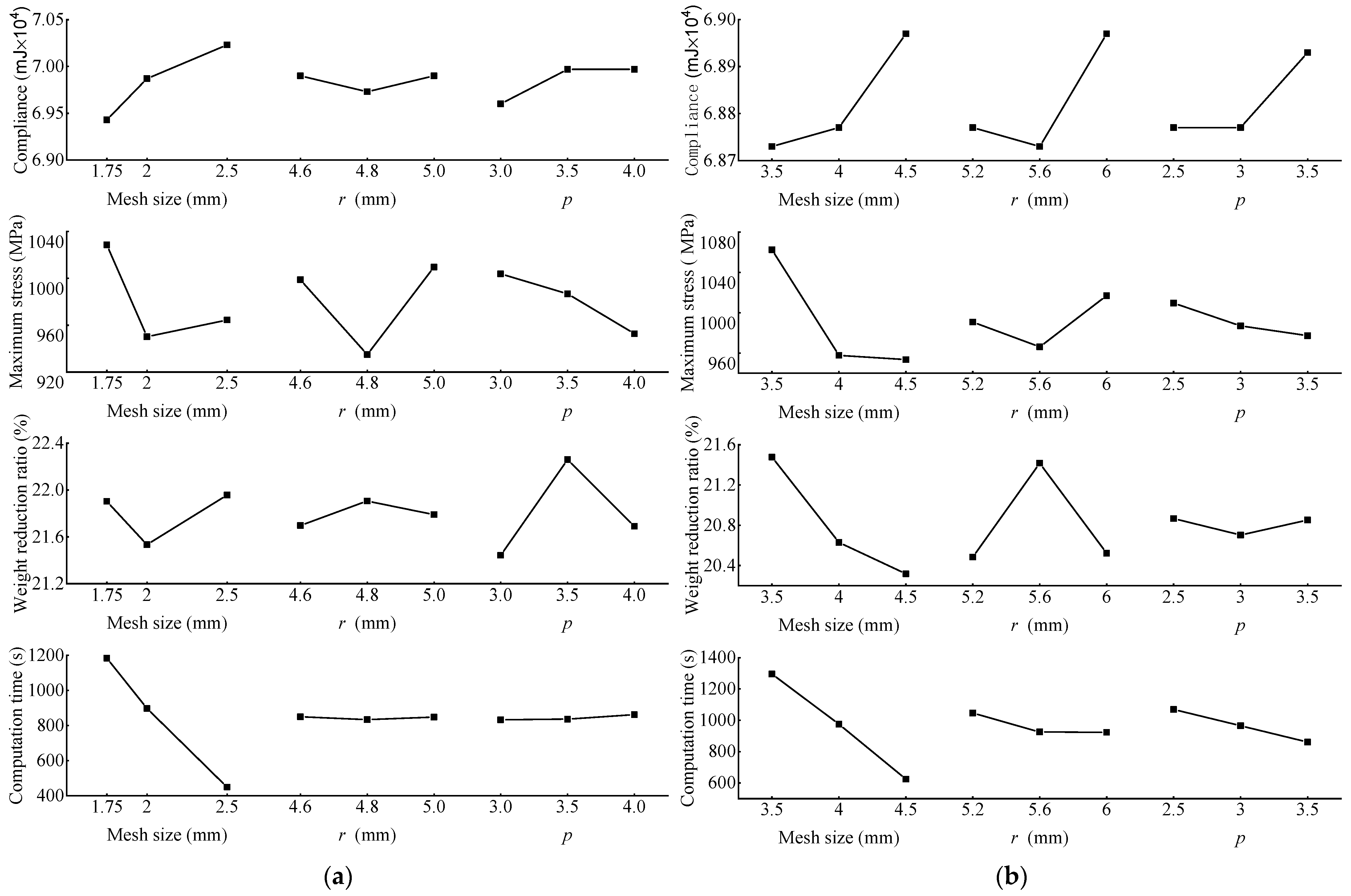
3.4. Mesh Size
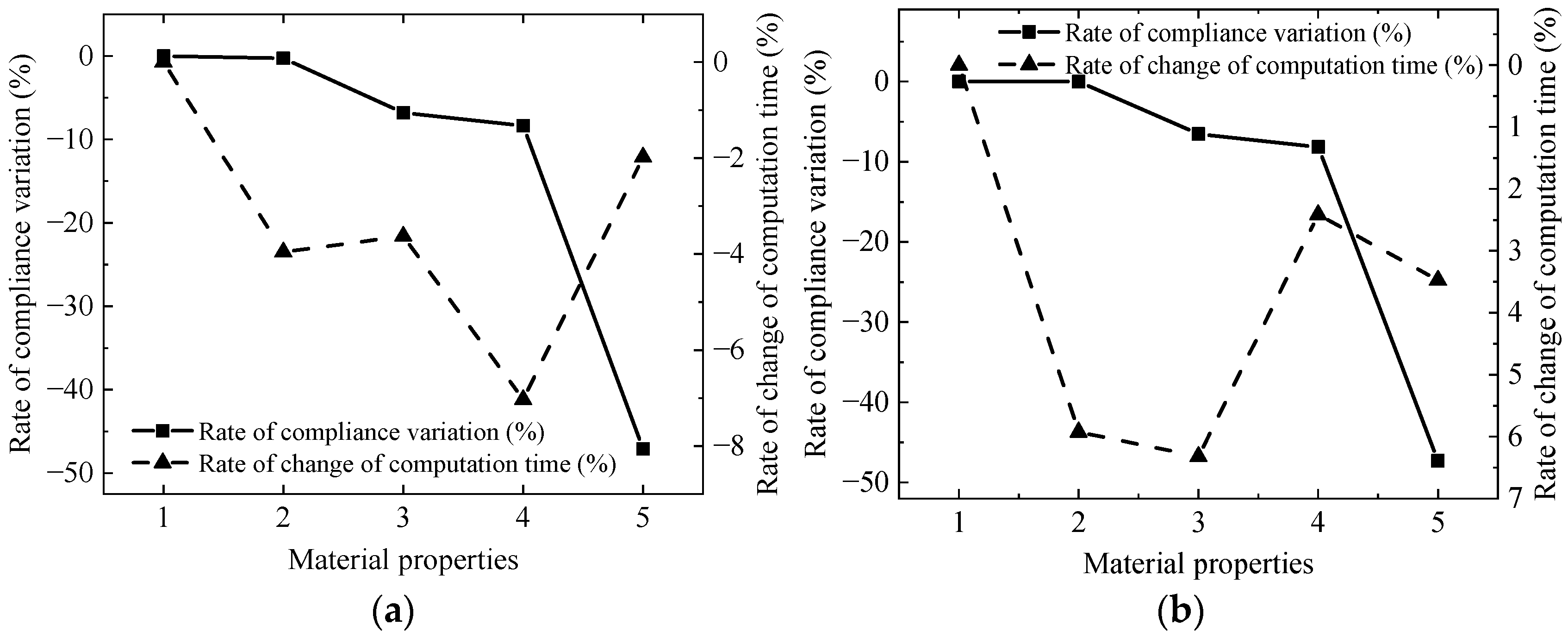
3.5. Material Properties
3.6. Initial Density
3.7. Filter Radius
3.8. Penalty Factor
4. Geometric Reconstruction of Topology Optimization Results
4.1. Geometric Reconstruction Criteria
- (1)
- Removal of isolated body features: Isolated body features are primarily caused by intermediate-density units generated by the variable density method of TO. These features do not contribute to structural performance improvements, but they can lead to mesh failure in the FEA and thereby an increase in ineffective branches during AM; hence, they must be eliminated.
- (2)
- Material removal from thin branches: Thin branches can be considered thin-walled features. Unless the structure design specifically requires thin-walled features, such a feature generally increases the need for a support material and could damage the surface quality during support material removal; thus, such features should be eliminated.
- (3)
- Material removal and connection of disconnected branches: The presence of disconnected branches suggests that they may become part of the optimal load transfer path. These disconnected branches should be extended and connected to ensure that the structural performance meets the loading requirements. If additional weight reduction is feasible, the elimination of this feature should be validated to see whether the loading requirements can still be met, thereby maximizing the benefits of weight reduction.
- (4)
- Transition treatment of sharp corner features: Metal-based AM technologies typically use lasers as energy sources, and their laser spots are approximately circular with a minimum focal diameter. For instance, EOS devices have laser spot diameters ranging from 40 to 100 µm, and the SLM solution devices range from 70 to 115 µm. Therefore, unless fine sharp corner features must be retained, sharp corners should undergo transition treatment to accommodate the physical characteristics of the laser spot and improve manufacturing quality.
- (5)
- Removal of closed internal hole features: During TO, intermediate-density units may lead to the creation of closed internal holes. Metal AM technologies using powder spreading or powder delivery methodologies are ineffective at removing powder particles inside internal holes, thus requiring secondary processing to eliminate them. This post-processing reduces structural performance and damages the surface quality. Therefore, the generation of closed internal hole features should be avoided as much as possible.
- (6)
- Ensuring machining allowance: Although SLM technology offers higher manufacturing precision than other metal AM technologies, regions requiring higher precision than the SLM capability (e.g., mating surfaces or fixed connection areas) must be reserved with a machining allowance to allow for subsequent surface finishing to improve surface smoothness.
- (7)
- Shape optimization of stress concentration regions: TO is conducted based on the existing geometric model, and its optimization results are constrained by geometric boundary conditions. For stress concentration areas placed at geometric boundaries, shape optimization should be performed during post-processing to lessen stress concentrations and enhance mechanical performance.
4.2. Geometric Reconstruction Approach
- Step 1:
- Adjust the MC algorithm’s isosurface threshold: By adjusting the isosurface threshold of the MC algorithm, the lower bound of the density value for intermediate-density units to be retained is controlled. The intermediate-density units above this lower bound are taken as the solid material, whereas those below it are considered the void material. This process lessens or eliminates the undesirable features resulting from TO under a given volume constraint that impacts structural performance.
- Step 2:
- Use PolyNURBS for solid fitting: The PolyNURBS method is commonly utilized to perform solid fitting on the TO structural configuration. During such a process, the pre-established geometric reconstruction criteria should be fully taken into account to ensure that the fitted structure meets the design requirements and optimizes performance.
- Step 3:
- Use SolidWorks for parametric modeling: In SolidWorks, parametric modeling is performed for non-design regions (such as ear flanges and bolt connection holes) to complement the structure generated by TO and complete the engineering design.
5. Simulation Experimental Results and Discussions
5.1. Simulation Protocol Based on the Orthogonal Experiment
5.2. Structural Configurations of Topology Optimization and Results of Geometric Reconstruction
5.3. Range and Variance Analyses
5.4. Comprehensive Balance Method Analysis
5.4.1. Hexahedral Mesh
5.4.2. Tetrahedral Mesh
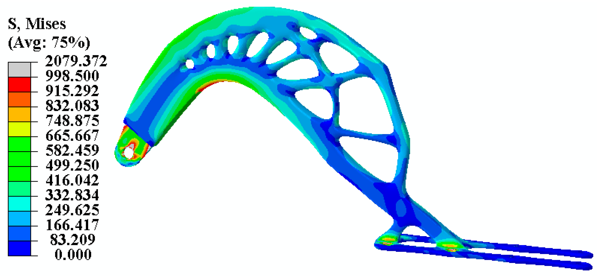
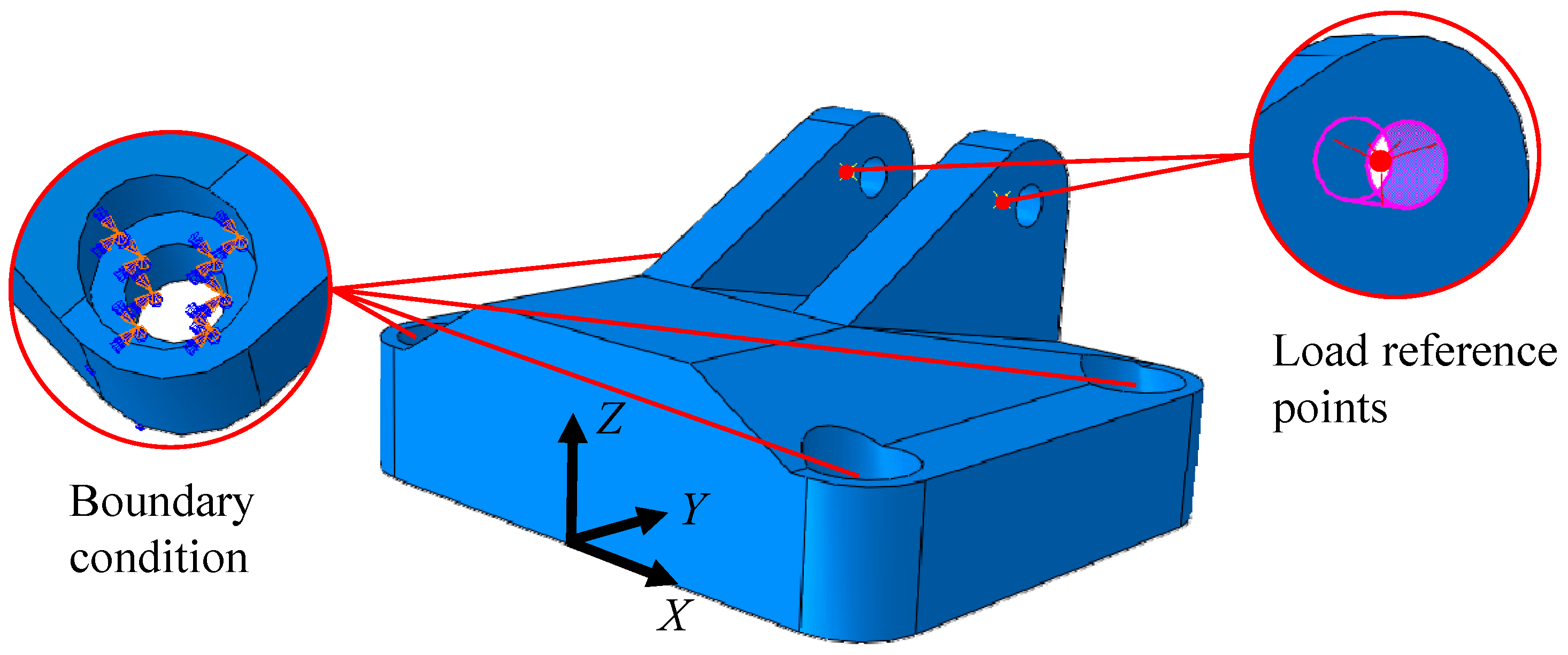
5.5. Validation of Recommended Criterias of TO: A Case Study of an Aircraft Bracket
6. Conclusions
Author Contributions
Funding
Institutional Review Board Statement
Informed Consent Statement
Data Availability Statement
Conflicts of Interest
References
- Ibhadode, O.; Zhang, Z.D.; Sixt, J.; Nsiempba, K.M.; Orakwe, J.; Martinez-Marchese, A.; Ero, O.; Shahabad, S.I.; Bonakdar, A.; Toyserkani, E. Topology optimization for metal additive manufacturing: Current trends, challenges, and future outlook. Virtual Phys. Prototyp. 2023, 18, e2181192. [Google Scholar] [CrossRef]
- Zhu, J.H.; Zhou, H.; Wang, C.; Zhou, L.; Yuan, S.Q.; Zhang, W.H. A review of topology optimization for additive manufacturing: Status and challenges. Chin. J. Aeronaut. 2021, 34, 91–110. [Google Scholar] [CrossRef]
- Bendsøe, M.P.; Ben-Tal, A.; Zowe, J. Optimization methods for truss geometry and topology design. Struct. Optim. 1994, 7, 141–159. [Google Scholar] [CrossRef]
- Bendsoe, M.P.; Kikuchi, N. Generating optimal topologies in structural design using a homogenization method. Comput. Methods Appl. Mech. Eng. 1988, 71, 197–224. [Google Scholar] [CrossRef]
- Tenek, L.H.; Hagiwara, I. Optimal rectangular plate and shallow shell topologies using thickness distribution or homogenization. Comput. Methods Appl. Mech. Eng. 1994, 115, 111–124. [Google Scholar] [CrossRef]
- Bendsøe, M.P.; Sigmund, O. Material interpolation schemes in topology optimization. Arch. Appl. Mech. 1999, 69, 635–654. [Google Scholar] [CrossRef]
- Xie, Y.M.; Steven, G.P. A simple evolutionary procedure for structural optimization. Comput. Struct. 1993, 49, 885–896. [Google Scholar] [CrossRef]
- Yang, X.Y.; Xie, Y.M.; Steven, G.P.; Querin, O.M. Bidirectional evolutionary method for stiffness optimization. AIAA J. 1999, 37, 1483–1488. [Google Scholar] [CrossRef]
- Guo, X.; Zhang, W.S.; Zhong, W.L. Doing topology optimization explicitly and geometrically-a new moving morphable components based framework. J. Appl. Mech.-Trans. ASME 2014, 81, 081009. [Google Scholar] [CrossRef]
- Wang, M.Y.; Wang, X.; Guo, D. A level set method for structural topology optimization. Comput. Methods Appl. Mech. Eng. 2003, 192, 227–246. [Google Scholar] [CrossRef]
- Huang, X. On smooth or 0/1 designs of the fixed-mesh element-based topology optimization. Adv. Eng. Softw. 2021, 151, 102942. [Google Scholar] [CrossRef]
- Huang, X. Smooth topological design of structures using the floating projection. Eng. Struct. 2020, 208, 110330. [Google Scholar] [CrossRef]
- Huang, X.D.; Li, W.B. Three-field floating projection topology optimization of continuum structures. Comput. Methods Appl. Mech. Eng. 2022, 399, 115444. [Google Scholar] [CrossRef]
- Fu, Y.F.; Rolfe, B.; Chiu, L.N.S.; Wang, Y.N.; Huang, X.D.; Ghabraie, K. SEMDOT: Smooth-edged material distribution for optimizing topology algorithm. Adv. Eng. Softw. 2020, 150, 102921. [Google Scholar] [CrossRef]
- Sui, Y.K.; Du, J.Z.; Guo, Y.Q. Independent continuous mapping for topological optimization of frame structures. ACTA Mech. Sin. 2006, 22, 611–619. [Google Scholar] [CrossRef]
- Rozvany, G.I.N. A critical review of established methods of structural topology optimization. Struct. Multidiscip. Optim. 2009, 37, 217–237. [Google Scholar] [CrossRef]
- Diaz, A.; Sigmund, O. Checkerboard patterns in layout optimization. Struct. Optim. 1995, 10, 40–45. [Google Scholar] [CrossRef]
- Haber, R.B.; Jog, C.S.; Bendsoe, M.P. A new approach to variable-topology shape design using a constraint on perimeter. Struct. Optim. 1996, 11, 1–12. [Google Scholar] [CrossRef]
- Sigmund, O. Design of Material Structures Using Topology Optimization. Ph.D. Thesis, Technical University of Denmark Lyngby, Kongens Lyngby, Denmark, 1994. [Google Scholar]
- Bendsøe, M.P. Optimization of Structural Topology, Shape, and Material; Springer: Berlin/Heidelberg, Germany, 1995; Volume 414. [Google Scholar]
- Svanberg, K. The method of moving asymptotes—A new method for structural optimization. Int. J. Numer. Methods Eng. 1987, 24, 359–373. [Google Scholar] [CrossRef]
- Wang, Q.L.; Han, H.T.; Wang, C.; Liu, Z.Y. Topological control for 2D minimum compliance topology optimization using SIMP method. Struct. Multidiscip. Optim. 2022, 65, 38. [Google Scholar] [CrossRef]
- Da Silveira, O.A.A.; Palma, L.F. Some considerations on multi-material topology optimization using ordered SIMP. Struct. Multidiscip. Optim. 2022, 65, 261. [Google Scholar] [CrossRef]
- Chen, Y.L. Metal Additive-Manufactured Joints for Spatial Structures: Topology Optimization. Master’s Thesis, Zhejiang University, Hangzhou, China, 2020. [Google Scholar]
- Ramos, A.; Angel, V.G.; Siqueiros, M.; Sahagun, T.; Gonzalez, L.; Ballesteros, R. Reviewing additive manufacturing techniques: Material trends and weight optimization possibilities through innovative printing patterns. Materials 2025, 18, 1377. [Google Scholar] [CrossRef] [PubMed]
- Moura, B.; Monteiro, H. Current development of the metal additive manufacturing sustainability—A systematic review. Environ. Impact Assess. Rev. 2025, 112, 107778. [Google Scholar] [CrossRef]
- Chuang, C.-H.; Chen, S.; Yang, R.-J.; Vogiatzis, P. Topology optimization with additive manufacturing consideration for vehicle load path development. Int. J. Numer. Methods Eng. 2018, 113, 1434–1445. [Google Scholar] [CrossRef]
- Zou, J.; Zhang, Y.C.; Feng, Z.Y. Topology optimization for additive manufacturing with self-supporting constraint. Struct. Multidiscip. Optim. 2021, 63, 2341–2353. [Google Scholar] [CrossRef]
- Azevedo, A.S.D.; Li, H.; Ishida, N.; Siqueira, L.O.; Cortez, R.L.; Silva, E.C.N.; Nishiwaki, S.; Picelli, R. Body-fitted topology optimization via integer linear programming using surface capturing techniques. Int. J. Numer. Methods Eng. 2024, 125, e7480. [Google Scholar] [CrossRef]
- Wu, X.C.; Shen, H.P.; Zhang, T.Y.; Li, H.Y.; Liu, B.G.; Yan, S.D. Research on a boundary regularization geometric reconstruction method of topology optimization structure based on the Freeman code. Adv. Mech. Eng. 2023, 15. [Google Scholar] [CrossRef]
- Zirak, N.; Shirinbayan, M.; Deligant, M.; Tcharkhtchi, A. Toward polymeric and polymer composites impeller fabrication. Polymers 2022, 14, 97. [Google Scholar] [CrossRef]
- Shakeria, Z.; Benfriha, K.; Zirak, N.; Shirinbayan, M. Optimization of FFF processing parameters to improve geometrical accuracy and mechanical behavior of polyamide 6 using grey relational analysis (GRA). Preprint 2021. [Google Scholar] [CrossRef]
- Ahmadifar, M.; Benfriha, K.; Shirinbayan, M. Thermal, tensile and fatigue behaviors of the PA6, short carbon fiber-reinforced PA6, and continuous glass fiber-reinforced PA6 materials in fused filament fabrication (FFF). Polymers 2023, 15, 507. [Google Scholar] [CrossRef]
- Dong, Z.; Han, C.J.; Liu, G.Q.; Zhang, J.; Li, Q.L.; Zhao, Y.Z.; Wu, H.; Yang, Y.Q.; Wang, J.H. Revealing anisotropic mechanisms in mechanical and degradation properties of zinc fabricated by laser powder bed fusion additive manufacturing. J. Mater. Sci. Technol. 2025, 214, 87–104. [Google Scholar] [CrossRef]
- Xiao, Z.F.; Yang, Y.Q.; Wang, D.; Song, C.H.; Bai, Y.C. Structural optimization design for antenna bracket manufactured by selective laser melting. Rapid Prototyp. J. 2018, 24, 539–547. [Google Scholar] [CrossRef]
- Seabra, M.; Azevedo, J.; Araújo, A.; Reis, L.; Pinto, E.; Alves, N.; Santos, R.; Mortágua, J.P. Selective laser melting (SLM) and topology optimization for lighter aerospace componentes. In Proceedings of the XV Portuguese Conference on Fracture, PCF 2016, Paco de Arcos, Portugal, 10–12 February 2016; pp. 289–296. [Google Scholar]
- Shi, G.H.; Guan, C.Q.; Quan, D.L.; Wu, D.T.; Tang, L.; Gao, T. An aerospace bracket designed by thermo-elastic topology optimization and manufactured by additive manufacturing. Chin. J. Aeronaut. 2020, 33, 1252–1259. [Google Scholar] [CrossRef]
- Bendsøe, M.P. Optimal shape design as a material distribution problem. Struct. Optim. 1989, 1, 193–202. [Google Scholar] [CrossRef]
- Zhou, M.; Rozvany, G.I.N. The COC algorithm, Part II: Topological, geometrical and generalized shape optimization. Comput. Methods Appl. Mech. Eng. 1991, 89, 309–336. [Google Scholar] [CrossRef]
- Stolpe, M.; Svanberg, K. An alternative interpolation scheme for minimum compliance topology optimization. Struct. Multidiscip. Optim. 2001, 22, 116–124. [Google Scholar] [CrossRef]
- Bruns, T.E.; Tortorelli, D.A. Topology optimization of non-linear elastic structures and compliant mechanisms. Comput. Methods Appl. Mech. Eng. 2001, 190, 3443–3459. [Google Scholar] [CrossRef]
- Svanberg, K. A class of globally convergent optimization methods based on conservative convex separable approximations. SIAM J. Optim. 2002, 12, 555–573. [Google Scholar] [CrossRef]
- Song, X.; Chen, L.B.; Shan, L.; Liu, Q.; Hu, Z.D. Design and implementation of static verification tests for additively manufactured civil aircraft components. J. Harbin Univ. Sci. Technol. 2022, 27, 70–78. [Google Scholar] [CrossRef]
- Bendsoe, M.P.; Sigmund, O. Topology Optimization: Theory, Methods, and Applications; Springer Science & Business Media: Berlin, Germany, 2013. [Google Scholar]
- Yamada, T.; Noguchi, Y. Topology optimization with a closed cavity exclusion constraint for additive manufacturing based on the fictitious physical model approach. Addit. Manuf. 2022, 52, 102630. [Google Scholar] [CrossRef]
- Biedermann, M.; Beutler, P.; Meboldt, M. Automated design of additive manufactured flow components with consideration of overhang constraint. Addit. Manuf. 2021, 46, 102119. [Google Scholar] [CrossRef]
- Newman, T.S.; Yi, H. A survey of the marching cubes algorithm. Comput. Graph. 2006, 30, 854–879. [Google Scholar] [CrossRef]
- Lorensen, W.E.; Cline, H.E. Marching cubes: A high resolution 3D surface construction algorithm. In Proceedings of the 14th Annual Conference on Computer Graphics and Interactive Techniques, Anaheim, CA, USA, 27–31 July 1987; Association for Computing Machinery: New York, NY, USA, 1987; pp. 163–169. [Google Scholar]
- Plackett, R.L.; Burman, J.P. The design of optimum multifactorial experiments. Biometrika 1946, 33, 305–325. [Google Scholar] [CrossRef]
- Box, G.E.P.; Wilson, K.B. On the experimental attainment of optimum conditions. J. R. Stat. Soc. Ser. B-Stat. Methodol. 1951, 13, 1–45. [Google Scholar] [CrossRef]
- Lewis, R.W.; Zheng, Y. Coarse optimization for complex systems: An application of orthogonal experiments. Comput. Methods Appl. Mech. Eng. 1992, 94, 63–92. [Google Scholar] [CrossRef]
- Yin, W.; Zhou, G.; Liu, D.; Meng, Q.; Zhang, Q.; Jiang, T. Numerical simulation and application of entrainment dust collector for fully mechanized mining support based on orthogonal test method. Powder Technol. 2021, 380, 553–566. [Google Scholar] [CrossRef]
- Sun, G.Y.; Li, G.Y.; Gong, Z.H.; Cui, X.Y.; Yang, X.J.; Li, Q. Multiobjective robust optimization method for drawbead design in sheet metal forming. Mater. Des. 2010, 31, 1917–1929. [Google Scholar] [CrossRef]
- Murphy, C.; Meisel, N.; Simpson, T.; McComb, C. Using autoencoded voxel patterns to predict part mass, required support material, and build time. In Proceedings of the 29th Annual International Solid Freeform Fabrication Symposium—An Additive Manufacturing Conference, SFF 2018, Austin, TX, USA, 13–15 August 2018; pp. 1660–1674. [Google Scholar]


| (%) | Hexahedral Mesh | Tetrahedral Mesh | (%) | Hexahedral Mesh | Tetrahedral Mesh |
|---|---|---|---|---|---|
| 10 |  |  | 60 |  |  |
| 20 |  |  | 70 |  |  |
| 30 |  |  | 80 |  |  |
| 40 |  |  | 90 |  |  |
| 50 |  |  | 100 |  |  |
| Mesh Size (mm) | Hexahedral Mesh | Mesh Size (mm) | Hexahedral Mesh | Mesh Size (mm) | Tetrahedral Mesh | Mesh Size (mm) | Tetrahedral Mesh |
|---|---|---|---|---|---|---|---|
| 14 |  | 3.5 |  | 14 |  | 4.5 |  |
| 10 |  | 3 |  | 10 |  | 4 |  |
| 6 |  | 2.5 |  | 8 |  | 3.5 |  |
| 5.5 |  | 2 |  | 6 |  | 3 |  |
| 5 |  | 1.75 |  | 5.5 |  | 2.5 |  |
| 4.5 |  | 1.5 |  | 5 |  | 2.25 |  |
| 4 |  | 1.25 |  |
| No. | Material Properties | Hexahedral Mesh | Tetrahedral Mesh |
|---|---|---|---|
| 1 | E = 110.3 GPa; = 0.31 |  |  |
| 2 | E = 110.3 GPa; = 0.33 |  |  |
| 3 | E = 118 GPa; = 0.33 |  |  |
| 4 | E = 120 GPa; = 0.342 |  |  |
| 5 | E = 209 GPa; = 0.269 |  |  |
| xinitial | Hexahedral | Tetrahedral | xinitial | Hexahedral | Tetrahedral |
|---|---|---|---|---|---|
| 0.1 |  |  | 0.6 |  |  |
| 0.2 |  |  | 0.7 |  |  |
| 0.3 |  |  | 0.8 |  |  |
| 0.4 |  |  | 0.9 |  |  |
| 0.5 |  |  | 1.0 |  |  |
| r (mm) | Hexahedral Mesh | r (mm) | Hexahedral Mesh | r (mm) | Tetrahedral Mesh | r (mm) | Tetrahedral Mesh |
|---|---|---|---|---|---|---|---|
| 0.5 |  | 3.4 |  | 0.25 |  | 6.4 |  |
| 1.0 |  | 3.6 |  | 0.5 |  | 6.8 |  |
| 2.0 |  | 3.8 |  | 1.0 |  | 7.2 |  |
| 2.2 |  | 4.0 |  | 2.0 |  | 7.6 |  |
| 2.4 |  | 4.2 |  | 4.0 |  | 8.0 |  |
| 2.6 |  | 4.4 |  | 4.4 |  | 8.4 | 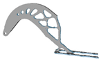 |
| 2.8 |  | 4.6 |  | 4.8 |  | 8.8 | 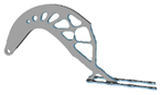 |
| 3.0 |  | 4.8 |  | 5.2 |  | 9.2 |  |
| 3.2 |  | 5.0 |  | 5.6 |  | 9.6 |  |
| 6.0 |  | 10 | 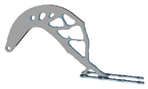 |
| p | Hexahedral Mesh | Tetrahedral Mesh | p | Hexahedral Mesh | Tetrahedral Mesh |
|---|---|---|---|---|---|
| 1.0 |  |  | 4.0 | 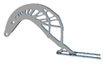 |  |
| 2.0 |  |  | 5.0 |  |  |
| 2.5 |  |  | 6.0 |  |  |
| 3.0 |  |  | 9.0 |  | - |
| 3.5 |  |  | 10 |  | - |
| Mesh Type | Level No. | Factor Level | ||
|---|---|---|---|---|
| C | D | E | ||
| Hexahedral | 1 | 1.75 | 4.6 | 3 |
| 2 | 2 | 4.8 | 3.5 | |
| 3 | 2.5 | 5 | 4 | |
| Tetrahedral | 1 | 3.5 | 5.2 | 2.5 |
| 2 | 4 | 5.6 | 3 | |
| 3 | 4.5 | 6 | 3.5 | |
| No. | Hexahedral | Tetrahedral | ||||
|---|---|---|---|---|---|---|
| C | D | E | C | D | E | |
| 1 | 1.75 | 4.80 | 4.00 | 3.5 | 6.0 | 3.0 |
| 2 | 1.75 | 5.00 | 3.50 | 3.5 | 5.2 | 2.5 |
| 3 | 1.75 | 4.60 | 3.00 | 3.5 | 5.6 | 3.5 |
| 4 | 2.00 | 5.00 | 4.00 | 4.0 | 5.2 | 3.0 |
| 5 | 2.00 | 4.80 | 3.00 | 4.0 | 6.0 | 3.5 |
| 6 | 2.00 | 4.60 | 3.50 | 4.0 | 5.6 | 2.5 |
| 7 | 2.50 | 5.00 | 3.00 | 4.5 | 5.2 | 3.5 |
| 8 | 2.50 | 4.60 | 4.00 | 4.5 | 6.0 | 2.5 |
| 9 | 2.50 | 4.80 | 3.50 | 4.5 | 5.6 | 3.0 |
| No. | Hexahedral Mesh | Tetrahedral Mesh | ||
|---|---|---|---|---|
| Structural Configuration | Geometric Configuration | Structural Configuration | Geometric Configuration | |
| 1 |  |  |  |  |
| 2 |  |  |  |  |
| 3 |  |  |  |  |
| 4 |  |  |  |  |
| 5 |  |  |  |  |
| 6 |  |  |  |  |
| 7 |  |  |  |  |
| 8 |  |  |  |  |
| 9 |  |  |  |  |
| Mesh Type | No. | Factor Level | Compliance (mJ × 104) | Maximum Stress (MPa) | Number of Iterations | Computation Time (s) | Weight Reduction Ratio (%) | ||
|---|---|---|---|---|---|---|---|---|---|
| C | D | E | |||||||
| Hexahedral | 1 | 1.75 | 4.80 | 4.00 | 6.94 | 896.2 | 36 | 1166 | 20.95 |
| 2 | 1.75 | 5.00 | 3.50 | 6.95 | 1095.7 | 37 | 1195 | 22.38 | |
| 3 | 1.75 | 4.60 | 3.00 | 6.94 | 1055.3 | 37 | 1189 | 22.38 | |
| 4 | 2.00 | 5.00 | 4.00 | 7.02 | 975.2 | 35 | 931 | 22.35 | |
| 5 | 2.00 | 4.80 | 3.00 | 6.94 | 959.6 | 38 | 900 | 21.31 | |
| 6 | 2.00 | 4.60 | 3.50 | 7.00 | 915.7 | 36 | 862 | 20.94 | |
| 7 | 2.50 | 5.00 | 3.00 | 7.00 | 957.7 | 38 | 460 | 20.64 | |
| 8 | 2.50 | 4.60 | 4.00 | 7.03 | 986.7 | 35 | 447 | 21.77 | |
| 9 | 2.50 | 4.80 | 3.50 | 7.04 | 948.8 | 36 | 442 | 23.46 | |
| Tetrahedral | 1 | 3.5 | 6.0 | 3.0 | 6.88 | 1108.4 | 40 | 1232 | 21.03 |
| 2 | 3.5 | 5.2 | 2.5 | 6.87 | 1080.9 | 49 | 1490 | 21.18 | |
| 3 | 3.5 | 5.6 | 3.5 | 6.87 | 998.5 | 38 | 1164 | 22.22 | |
| 4 | 4.0 | 5.2 | 3.0 | 6.86 | 928.0 | 40 | 1070 | 20.29 | |
| 5 | 4.0 | 6.0 | 3.5 | 6.91 | 969.8 | 37 | 837 | 20.36 | |
| 6 | 4.0 | 5.6 | 2.5 | 6.86 | 975.1 | 46 | 1017 | 21.24 | |
| 7 | 4.5 | 5.2 | 3.5 | 6.90 | 963.1 | 38 | 580 | 19.98 | |
| 8 | 4.5 | 6.0 | 2.5 | 6.90 | 972.7 | 46 | 699 | 20.18 | |
| 9 | 4.5 | 5.6 | 3.0 | 6.89 | 924.5 | 39 | 595 | 20.79 | |
| Indicator | Hexahedral Mesh | Tetrahedral Mesh | ||||||
|---|---|---|---|---|---|---|---|---|
| C | D | E | C | D | E | |||
| Compliance (mJ × 104) | km | k1 | 6.943 | 6.990 | 6.960 | 6.873 | 6.877 | 6.877 |
| k2 | 6.987 | 6.973 | 6.997 | 6.877 | 6.873 | 6.877 | ||
| k3 | 7.023 | 6.990 | 6.997 | 6.897 | 6.897 | 6.893 | ||
| R | 0.08 | 0.017 | 0.037 | 0.024 | 0.024 | 0.016 | ||
| SST | 0.010 | 0.001 | 0.003 | 0.001 | 0.001 | 0.001 | ||
| p | 0.107 | 0.675 | 0.301 | 0.232 | 0.232 | 0.342 | ||
| Optimal level | C1 | D2 | E1 | C1 | D2 | E1(E2) | ||
| Primary and secondary factors | C > E > D | C = D > E | ||||||
| Optimal solutions | C1E1D2 | C1D2E1(C1D2E2) | ||||||
| Maximum stress (MPa) | km | k1 | 1028.667 | 998.833 | 1003.800 | 1062.600 | 990.667 | 1009.567 |
| k2 | 950.167 | 934.867 | 986.733 | 957.633 | 966.033 | 986.967 | ||
| k3 | 964.400 | 1009.533 | 952.700 | 953.433 | 1016.967 | 977.133 | ||
| R | 78.5 | 74.666 | 51.1 | 109.167 | 50.934 | 32.434 | ||
| SST | 10,495.042 | 9781.336 | 4060.749 | 22,953.002 | 3892.696 | 1659.376 | ||
| p | 0.591 | 0.608 | 0.789 | 0.136 | 0.482 | 0.686 | ||
| Optimal level | C2 | D2 | E3 | C3 | D2 | E3 | ||
| Primary and secondary factors | C > D > E | C > D > E | ||||||
| Optimal solutions | C2D2E3 | C3D2E3 | ||||||
| Weight reduction ratio (%) | km | k1 | 21.903 | 21.697 | 21.443 | 21.477 | 20.483 | 20.867 |
| k2 | 21.533 | 21.907 | 22.260 | 20.630 | 21.417 | 20.703 | ||
| k3 | 21.957 | 21.790 | 21.690 | 20.317 | 20.523 | 20.853 | ||
| R | 0.424 | 0.21 | 0.817 | 1.16 | 0.934 | 0.164 | ||
| SST | 0.319 | 0.066 | 1.053 | 2.161 | 1.671 | 0.049 | ||
| p | 0.944 | 0.988 | 0.835 | 0.017 | 0.021 | 0.426 | ||
| Optimal level | C3 | D2 | E2 | C1 | D2 | E1 | ||
| Primary and secondary factors | E > C > D | C > D > E | ||||||
| Optimal solutions | E2C3D2 | C1D2E1 | ||||||
| Computation time (s) | km | k1 | 1183.333 | 849.667 | 832.667 | 1295.333 | 1046.667 | 1068.667 |
| k2 | 897.667 | 833.000 | 836.000 | 974.667 | 925.333 | 965.667 | ||
| k3 | 449.667 | 848.000 | 862.000 | 624.667 | 922.667 | 860.333 | ||
| R | 733.666 | 16.667 | 29.333 | 670.666 | 124 | 208.334 | ||
| SST | 820,576.222 | 505.556 | 1547.556 | 675,120.889 | 30,104.889 | 65,106.889 | ||
| p | 0.001 | 0.387 | 0.659 | 0.003 | 0.067 | 0.032 | ||
| Optimal level | C3 | D2 | E1 | C3 | D3 | E3 | ||
| Primary and secondary factors | C > E > D | C > E > D | ||||||
| Optimal solutions | C3E1D2 | C3E3D3 | ||||||
| Parameter | Original Model | Model in Ref. [43] | The Best Overall Solution | |
|---|---|---|---|---|
| Hexahedral Test 9 | Tetrahedral Test 3 | |||
| Volume (mm3) | 281,544 | 226,899 | 215,427 | 218,913 |
| Weight reduction ratio (%) | 0 | 19.38 | 23.46 | 22.22 |
| Maximum stress (MPa) | 1332.3 | 1094.9 | 948.8 | 998.5 |
Disclaimer/Publisher’s Note: The statements, opinions and data contained in all publications are solely those of the individual author(s) and contributor(s) and not of MDPI and/or the editor(s). MDPI and/or the editor(s) disclaim responsibility for any injury to people or property resulting from any ideas, methods, instructions or products referred to in the content. |
© 2025 by the authors. Licensee MDPI, Basel, Switzerland. This article is an open access article distributed under the terms and conditions of the Creative Commons Attribution (CC BY) license (https://creativecommons.org/licenses/by/4.0/).
Share and Cite
Chen, L.; Zhou, D. Analysis of Numerical Instability Factors and Geometric Reconstruction in 3D SIMP-Based Topology Optimization Towards Enhanced Manufacturability. Appl. Sci. 2025, 15, 6195. https://doi.org/10.3390/app15116195
Chen L, Zhou D. Analysis of Numerical Instability Factors and Geometric Reconstruction in 3D SIMP-Based Topology Optimization Towards Enhanced Manufacturability. Applied Sciences. 2025; 15(11):6195. https://doi.org/10.3390/app15116195
Chicago/Turabian StyleChen, Longbao, and Ding Zhou. 2025. "Analysis of Numerical Instability Factors and Geometric Reconstruction in 3D SIMP-Based Topology Optimization Towards Enhanced Manufacturability" Applied Sciences 15, no. 11: 6195. https://doi.org/10.3390/app15116195
APA StyleChen, L., & Zhou, D. (2025). Analysis of Numerical Instability Factors and Geometric Reconstruction in 3D SIMP-Based Topology Optimization Towards Enhanced Manufacturability. Applied Sciences, 15(11), 6195. https://doi.org/10.3390/app15116195