Reconstruction of a 3D Real-World Coordinate System and a Vascular Map from Two 2D X-Ray Pixel Images for Operation of Magnetic Medical Robots

Abstract

We propose a method to reconstruct a 3D coordinate system and a vascular map for the operation of magnetic medical robots (MMRs) controlled by a magnetic navigation system (MNS) using two 2D X-ray images and four corners of an MNS. Utilizing the proposed method, we calculated the relative rotation angle of a C-arm considering its rotational precision error. We derived the position information and 3D coordinate system of an MNS workspace in which the magnetic fields are generated and controlled by an MNS. The proposed method can also be utilized to reconstruct vascular maps. Reconstructed vascular maps are in the 3D coordinate system of the C-arm and can be transformed into the 3D coordinate system of an MNS workspace to generate the magnetic flux density with the desired direction and magnitude at the position of the MMR. The proposed method allows us to remotely and precisely control the MMR inserted into the vessel by controlling the external magnetic field. The proposed method was validated through in vitro experiments with an MNS mock-up and a vascular jig. Finally, the proposed method was applied to in vivo experiments where the MMR was inserted into the superficial femoral artery of a mini pig to remotely control the motion of the MMR. This research will enable precise and effective control of MMRs in various medical procedures utilizing an MNS.

1. Introduction

Magnetic medical robots (MMRs) contain permanent magnets and perform medical functions in the human tubular system by controlling an external magnetic field generated by a magnetic navigation system (MNS). MMRs utilize the magnetic characteristics in which the permanent magnet tends to be aligned along the direction of the external magnetic field and propelled along its gradient. Many researchers have developed various MMRs that can perform medical treatments and diagnoses through diverse designs and control mechanisms [1,2,3,4]. The MNS generates a magnetic field through permanent magnets, coils, and electromagnets which are placed around the target lesion [5,6,7]. The workspace of an MNS can be defined as a certain volume in which the magnetic field can be controlled to perform the medical functions of an MMR. To precisely control an MMR using an MNS, the 3D coordinate system of an MNS workspace has to be defined and the 3D position of an MMR in this coordinate system has to be identified to precisely generate the magnetic field, ensuring precise control of an MMR and increasing the success rate of medical functions. In many studies on robotic endovascular intervention using MMRs and MNSs, the 3D coordinate system of an MNS workspace was predefined utilizing multiple cameras fixed to MNSs or jigs [8,9,10,11]. However, in real clinical operation, medical doctors utilize a C-arm X-ray device to identify the blood vessel and endovascular devices such as guide wires and catheters along the blood vessel. X-ray images are 2D images and they cannot be directly applied to robotic endovascular intervention, which requires 3D real-world coordinates of both the location of an MMR and the blood vessel map in order to accurately apply magnetic field. To control an MMR using a C-arm X-ray device and an MNS, it is necessary to estimate a 3D vascular map from 2D X-ray images and to ensure compatibility between the commercial C-arm and the MNS. While Nguyen et al. extracted 3D positions of blood vessels using a dual C-arm embedded in an MNS [12], the studies to estimate the 3D positions of blood vessels by ensuring the compatibility between commercial C-arm X-ray devices and MNSs are limited.

Several researchers have reconstructed a 3D coordinate in X-ray imaging devices [13,14,15,16,17,18]. They captured two or more images from various views and calibrated intrinsic and extrinsic parameters of the C-arm. They derived intrinsic parameters such as focal length, principal point, and pixel size before the operation to reflect the geometric properties of the images. However, the extrinsic parameters, such as the rotation angle displayed on the control program of C-arm, may not be as accurate as expected, which can cause errors in the reconstruction of the vascular map. Many researchers have developed various methods to calibrate the extrinsic parameters of a C-arm. Movassaghi et al. [13] conducted a calibration procedure that utilizes calibration templates prior to the coronary modeling. However, it cannot consider the changes in extrinsic parameters during operation, requires a point matching process across multiple X-ray images, and shows a significant increase in error when the angular difference between the two images is less than 35° or greater than 145°. However, when using a commercial C-arm X-ray device and an MNS, the maximum angular difference between the two X-ray images is approximately 15°, making this method inapplicable. Other researchers proposed a method to derive the transformation between two uncalibrated X-ray images using the Levenberg–Marquardt (LM) algorithm [14]. However, it assumes that the C-arm images are acquired at orthogonal angles, converges slowly, and is sometimes trapped by local optima. To reduce convergence time, Fu et al. [15] proposed a two-stage LM algorithm. Nevertheless, the convergence speed of the LM algorithm still needs to be improved, and it is also vulnerable to geometric errors such as inaccuracies in the actual rotation angles of the C-arm. Meanwhile, many studies estimated extrinsic parameters using some specific landmark points in vessels such as bifurcations or end points [16,17]. These methods require additional steps to identify the landmark points and determine the correspondence between them in each image. Also, three or more images are still required to determine the unique correspondence of each landmark point [18].

Also, various methods have been developed to reconstruct a 3D vascular map that represents the centerline of the blood vessel in a 3D coordinate [14,15,17,19]. The LM algorithm used for the calibration of the external parameters was also used for the reconstruction of the centerlines of vessels [14,15]. However, the limitations of the LM algorithm of slow convergence and trapping in local optima also exist in the reconstruction process of a vascular map. Some researchers proposed a point cloud method to reconstruct a 3D vascular map [17]. This method utilizes multiple images and conducts iterative fitting of B-spline curve. Liao et al. [19] defined an energy function as the objective function which represents the difference between the data displayed in the images and the 3D coordinate, and reconstructed a 3D vascular map by minimizing the energy function through an α-expansion method. It has low computation cost and fast convergence time. However, the accuracy and computation cost of the α-expansion method are significantly affected by the initial Z coordinate at the beginning of computation because it iteratively searches for the optimal Z coordinate from the initial Z coordinate to minimize the energy function.

In this study, we propose a method to reconstruct a 3D coordinate system and a vascular map for the operation of an MMR controlled by an MNS using two X-ray images with restricted angles and four corners of an MNS. In Section 2.1, we outline the relationship between the 2D coordinates within the coordinate system of an X-ray image and the 3D coordinates within the coordinate system of a C-arm. In Section 2.2, we suggest a different viewpoint to describe the translation and rotation of a focal spot of a C-arm as the rotation of an object in a fixed coordinate system using the motion characteristic of a C-arm. In Section 2.3, we propose a transformation method from two 2D X-ray pixel images to a 3D real-world coordinate (TMPR) to obtain the coordinates of an object in a 3D coordinate system of a C-arm without the point matching process across multiple images. In Section 2.4, we propose a method to estimate the relative rotation angle between two views with four corners of an MNS using the TMPR, thereby compensating for rotational angle errors of a C-arm. In Section 2.5, we suggest a technique to calculate the centerline path of the blood vessel utilizing the TMPR. In Section 3, we validate the TMPR and propose reconstruction methods in an in vitro experiment using an MNS mock-up and a vascular jig. Finally, the effectiveness of the proposed methods is verified through in vivo experiments in the superficial femoral artery (SFA) of a mini pig, where an MMR is remotely operated by an MNS. This confirms that the TMPR can enhance the compatibility between a commercial C-arm X-ray device and an MNS in a constrained environment where the maximum angular difference between the two X-ray images is approximately 15°.

2. Concepts and Applications of TMPR

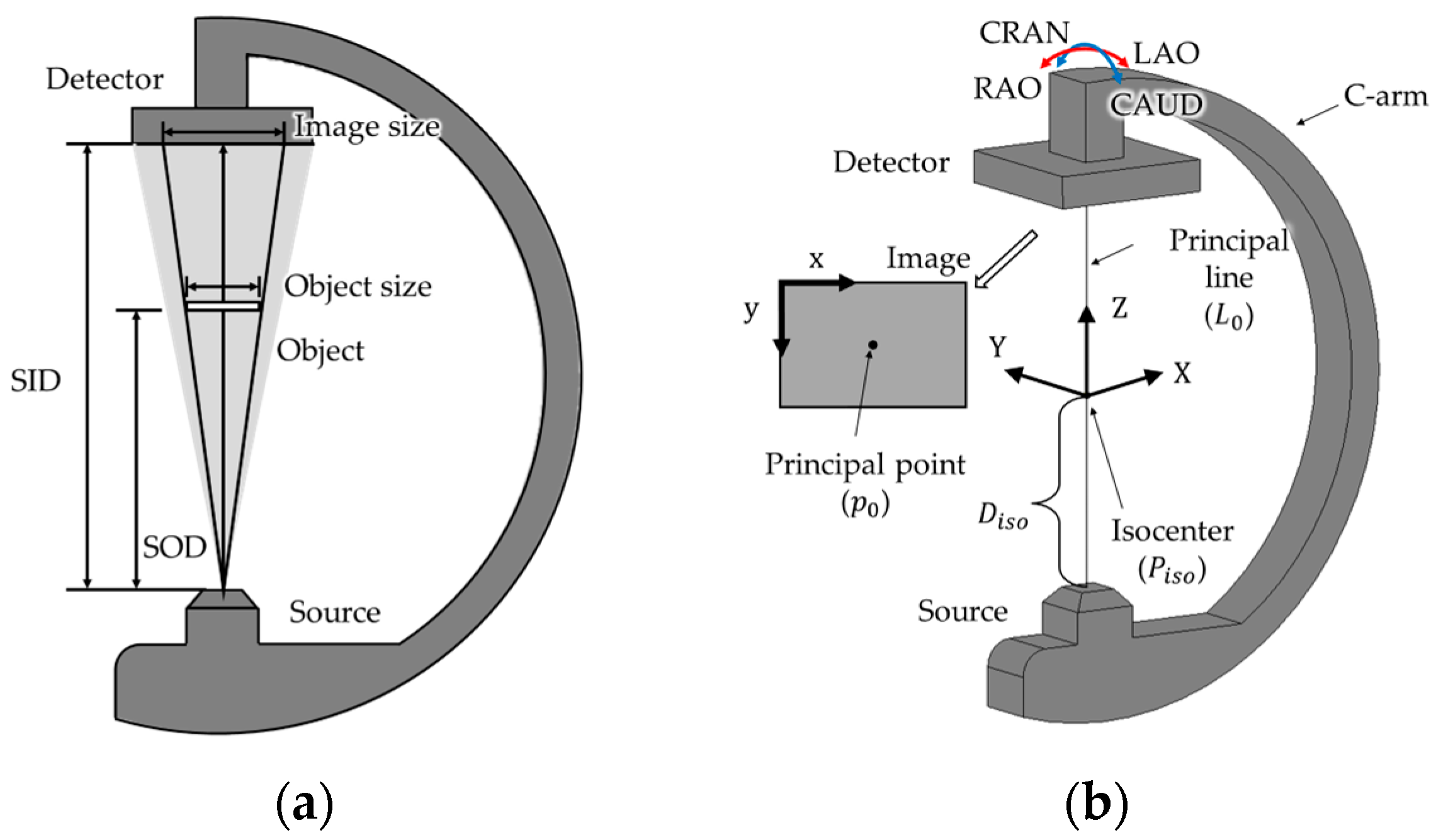
2.1. Magnification Characteristic of X-Ray Images

In this section, we formulate the projection between 2D coordinates on an X-ray image and 3D coordinates within a C-arm’s coordinate system, utilizing the magnification characteristic of X-ray images. A 2D coordinate of the X-ray image in Figure 1b is a 2D coordinate in the unit of pixels, with the origin located at the top-left corner of the image. A 3D coordinate of a C-arm is a 3D coordinate with a unit of length and defined by the X, Y, and Z axes, as illustrated in Figure 1b. As shown in Figure 1a,b, the source and detector are aligned parallel to each other at the opposite ends of a C-arm [20]. In this study, symbols for the points and lines are written in italic type, while symbols for the coordinates of points and lines are written in italic and bold type. The perpendicular line from the source to the detector is referred to as the principal line (L₀), and its foot of the perpendicular on the image is called the principal point (p₀). The isocenter (P_iso) is a point on the principal line and serves as the rotation center of the C-arm. The 3D coordinate system of the C-arm can be defined by setting P_iso as the origin, L₀ as the Z axis, the rotation axis in the RAO/LAO (right/left anterior oblique) direction as the Y axis, and the rotation axis in the CAUD/CRAN (caudal/cranial) direction as the X axis. An object captured by X-rays is magnified on the image. The magnification factor (MF) is the ratio between the image size and object size or between the SID (source to image distance) and SOD (source to object distance), as shown in Figure 1a and Equation (1) [21].

$$\mathrm{M}\mathrm{F}={\displaystyle \frac{\mathrm{I}\mathrm{m}\mathrm{a}\mathrm{g}\mathrm{e} \mathrm{s}\mathrm{i}\mathrm{z}\mathrm{e}}{\mathrm{O}\mathrm{b}\mathrm{j}\mathrm{e}\mathrm{c}\mathrm{t} \mathrm{s}\mathrm{i}\mathrm{z}\mathrm{e}}}={\displaystyle \frac{\mathrm{S}\mathrm{I}\mathrm{D}}{\mathrm{S}\mathrm{O}\mathrm{D}}}$$

(1)

The image size, object size, SID, and SOD in (1) have length units. If an object is represented by n_pixel pixels in the image and each pixel has a length of d_pixel, then the object size can be expressed as (2) in terms of n_pixel, d_pixel, Z, D_iso, SID, and SOD, which can be seen as follows:

$$\mathrm{O}\mathrm{b}\mathrm{j}\mathrm{e}\mathrm{c}\mathrm{t} \mathrm{s}\mathrm{i}\mathrm{z}\mathrm{e}={\displaystyle \frac{\mathrm{I}\mathrm{m}\mathrm{a}\mathrm{g}\mathrm{e} \mathrm{s}\mathrm{i}\mathrm{z}\mathrm{e}}{\mathrm{M}\mathrm{F}}}=n_{pixel}\times d_{pixel}\times {\displaystyle \frac{\mathrm{S}\mathrm{O}\mathrm{D}}{\mathrm{S}\mathrm{I}\mathrm{D}}}=n_{pixel}\times d_{pixel}\times {\displaystyle \frac{Z+D_{iso}}{\mathrm{S}\mathrm{I}\mathrm{D}}}$$

(2)

where D_iso represents the distance from the source to the P_iso, and Z is the difference between SOD and D_iso. We can obtain f(Z) in (3) after dividing (2) by n_pixel, which is the object size per pixel with a unit of mm/pixel. This shows the ratio between pixel units in the X-ray image and the length unit according to the Z coordinate in the 3D coordinate system of the C-arm.

$$f\left(Z\right)=d_{pixel}\times {\displaystyle \frac{Z+D_{iso}}{\mathrm{S}\mathrm{I}\mathrm{D}}}$$

(3)

For a point P located in 3D space, the relationship between the position of P in the 3D coordinate system of the C-arm and the position of p in the 2D coordinate system of the X-ray image is shown in (4) and (5). The p is the 2D point where the 3D point P is projected onto the X-ray image. Equations (4) and (5) are as follows:

$$\mathit{P}=\left[\begin{array}{c}X\\ Y\\ Z\end{array}\right]=\left[\begin{array}{c}\left(x-x_0\right)\times f\left(Z\right)\\ \left(y-y_0\right)\times f\left(Z\right)\\ Z\end{array}\right]$$

(4)

$$\mathit{p}=\left[\begin{array}{c}x\\ y\end{array}\right]={\displaystyle \frac{1}{f\left(Z\right)}}\left[\begin{array}{c}X\\ Y\end{array}\right]+\left[\begin{array}{c}{x}_0\\ y_0\end{array}\right]$$

(5)

where x₀ and y₀ represent the respective x and y coordinates of the principal point (p₀) in the 2D coordinate system of the X-ray image. Equation (4) shows that P in the 3D coordinate system of the C-arm corresponding to p in the 2D coordinate system of the X-ray image can be expressed as a function of Z when p is given. Currently, the feasible range of Z is −D_iso ≤ Z ≤ SID −D_iso. Equation (5) shows that when P is given the p that is a projected point of P onto the X-ray image can be calculated.

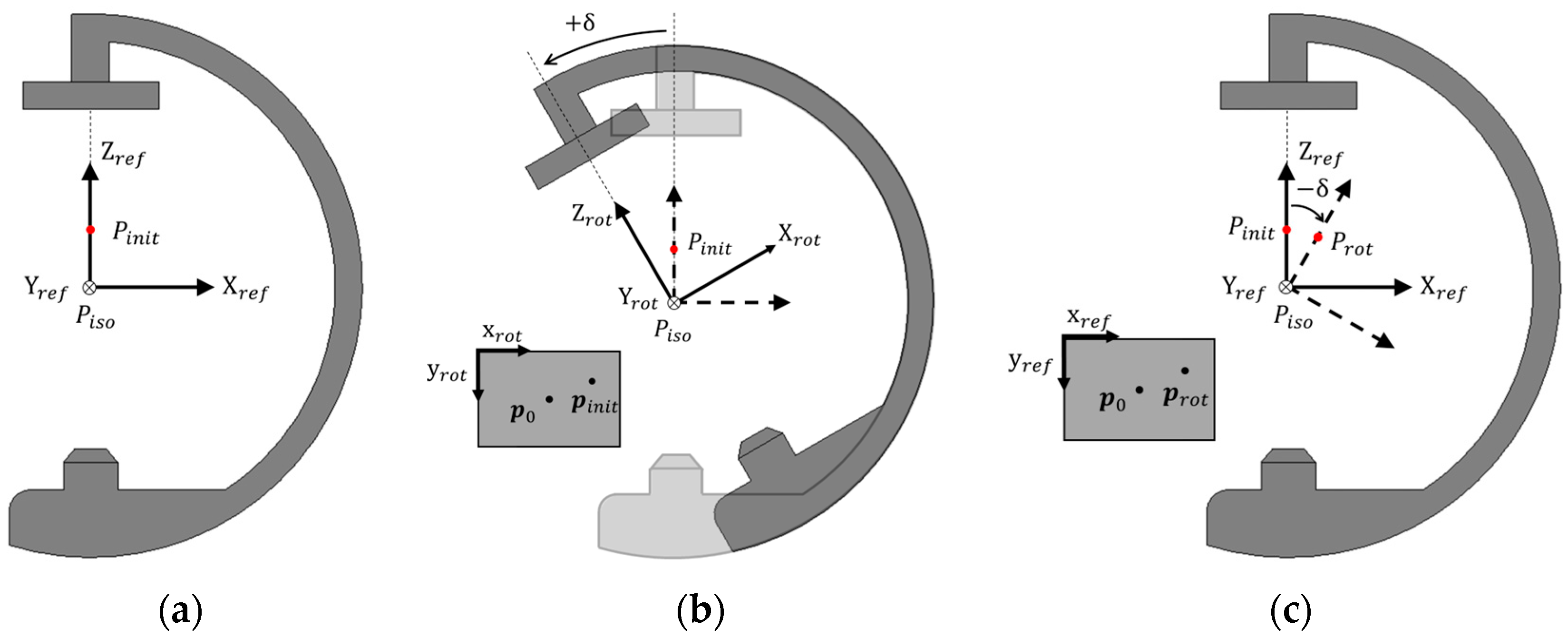
2.2. Motion Characteristic of the C-Arm

In previous studies, the origin of the 3D coordinate system of the C-arm is located at the focal spot. Therefore, the rotation of the C-arm is equivalent to the translation and rotation of the focal spot. As shown in Figure 2a, the initial 3D coordinate system of the C-arm with a rotation angle of 0, where the isocenter (P_iso) is the origin and the Z-axis is parallel to the principal line (L₀), is defined as C_ref. We assume that a point P_init exists in the C-arm workspace. When the C-arm rotates by δ about P_iso, as shown in Figure 2b, the rotated 3D coordinate system of the C-arm is defined by C_rot, of which the origin is also located at the P_iso and the position of P_init can be calculated with respect to C_rot. On the other hand, if the C_ref is fixed and P_init rotates by -δ about the P_iso, as shown in Figure 2c, we can define this rotated point as P_rot. The position of P_rot can be calculated with respect to C_ref. The position of P_init and P_rot in C_rot and C_ref are same, as shown in Figure 2b,c. Therefore, the images captured from each view should be identical. Consequently, the translation and rotation of the focal spots can be described solely by the rotation of an object about the P_iso in the fixed coordinate system by defining the P_iso as an origin of the 3D coordinate system of the C-arm. At this point, we do not consider the translation of the imaging equipment.

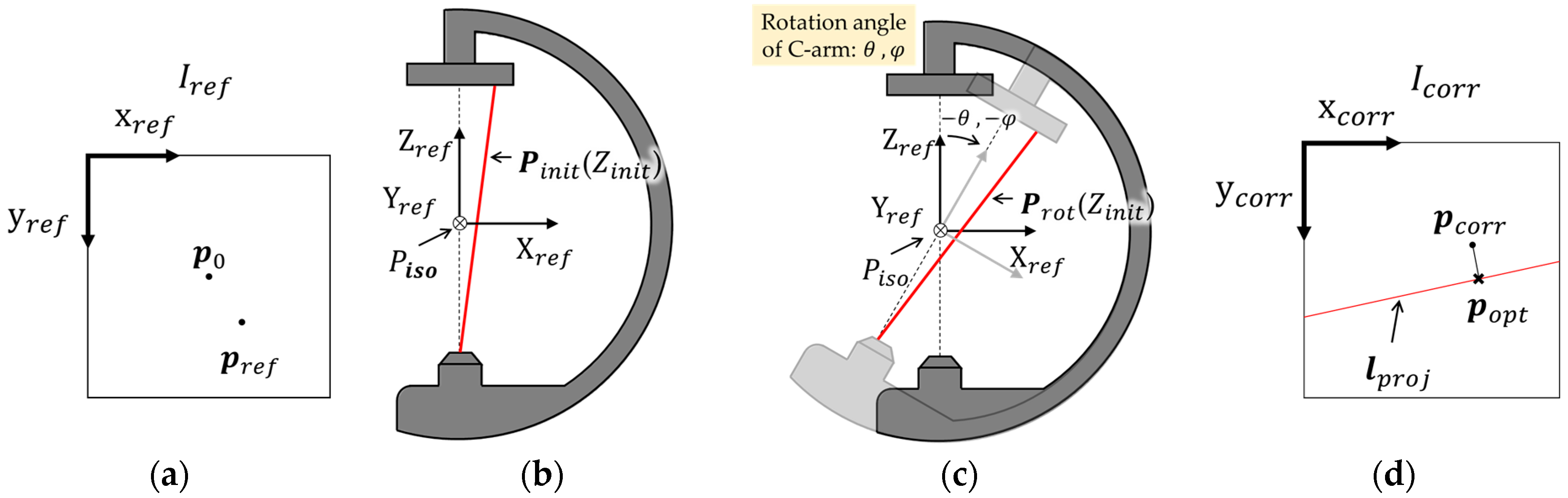
2.3. Transformation Method from Two 2D X-Ray Pixel Images to 3D Real-World Coordinates (TMPR)

In this section, we explain the detailed method to reconstruct the 3D coordinates from the two X-ray images. When two X-ray images are captured from different views, V_ref is the reference view obtained without rotating the C-arm and V_corr is the corresponding view obtained with rotating the C-arm. The 3D coordinates of V_ref are described with respect to C_ref. The 2D X-ray images captured from each view are I_ref and I_corr, and are depicted in Figure 3a,d. The projected pixel points of P in 3D space onto I_ref and I_corr are denoted as p_ref and p_corr. The coordinates of the principal points in I_ref and I_corr are defined as p₀. Figure 3a shows p_ref and p₀ in I_ref. The 3D coordinates of P_init = [X_init Y_init Z_init]^T in C_ref corresponding to p_ref can be derived utilizing (4), as shown in Figure 3a,b.

When the C-arm is rotated from V_ref to V_corr in the order of RAO/LAO by θ and in CAUD/CRAN by φ, we can calculate the coordinates P_rot = [X_rot Y_rot Z_rot]^T in C_ref by rotating P_init with respect to the P_iso by −θ and −φ in the same order, as shown in Figure 3b,c. Equation (6) is a rotational transformation matrix to transform P_init into P_rot, which can be calculated from (7) as follows:

$${\mathbf{R}}_{rot}=\left[\begin{array}{ccc}1& 0& 0\\ 0& \cos \phi & \sin \phi \\ 0& -\sin \phi & \cos \phi \end{array}\right]\left[\begin{array}{ccc}\cos \theta & 0& \sin \theta \\ 0& 1& 0\\ -\sin \theta & 0& \cos \theta \end{array}\right]$$

(6)

$${\mathit{P}}_{rot}={\mathbf{R}}_{rot}{\mathit{P}}_{init}=\left[\begin{array}{c}{X}_{rot}\left(Z_{init}\right)\\ Y_{rot}\left(Z_{init}\right)\\ Z_{rot}\left(Z_{init}\right)\end{array}\right]$$

(7)

where X_rot, Y_rot, and Z_rot of P_rot are functions of Z_init. We can calculate p_rot, which is projected onto I_corr, using (5) as follows:

$${\mathit{p}}_{rot}=\left[\begin{array}{c}{x}_{rot}\\ y_{rot}\end{array}\right]={\displaystyle \frac{1}{f\left(Z_{rot}\left(Z_{init}\right)\right)}}\left[\begin{array}{c}{X}_{rot}\left(Z_{init}\right)\\ Y_{rot}\left(Z_{init}\right)\end{array}\right]+\left[\begin{array}{c}{x}_0\\ y_0\end{array}\right]$$

(8)

Similarly to P_rot, each element of p_rot is also represented as a function of Z_init. In (8), both the numerator and denominator of each element of p_rot are the first-order functions of Z_init. After substituting 1/f(Z_rot(Z_init)) with g, as shown in (9), x_rot can be expressed as a function of g, as shown in (10). Finally, a linear relationship between x_rot and y_rot can be derived, as shown in (11):

$$g={\displaystyle \frac{1}{f\left(Z_{rot}\left(Z_{init}\right)\right)}}$$

(9)

$$x_{rot}=Ag+B$$

(10)

$$y_{rot}=Cg+D=E{x}_{rot}+F$$

(11)

where in (10) to (11), A, B, C, D, E, and F are real constants. The line represented by (11) is defined as l_proj, and each point on l_proj corresponds to 3D coordinates in C_ref. The closest point on l_proj to p_corr (foot of the perpendicular line) can be determined to p_opt by applying the soft epipolar line constraint [19]. The Z_init corresponding to p_opt can be calculated by (9) and (10). Z_init is later used as the initial value for the optimization process of the α-expansion method described in Section 2.5. Finally, we can calculate P_init in the 3D coordinates of the C-arm utilizing the calculated Z_init and p_ref in (4). In conclusion, we can determine the 3D coordinates of a point in the coordinate system of the C-arm from two 2D X-ray images captured from different views.

2.4. Calculation of a Relative Rotation Angle of the C-Arm Utilizing TMPR

In this section, we propose a method to estimate the relative rotation angle between two views. When we conduct an operation with an MNS, some corners of the structure can be captured in X-ray images. We can calculate the 3D coordinates of these corners with respect to given relative rotation angle of the C-arm, utilizing the TMPR. If the actual distances between corners are known, these can be utilized as the constraints to estimate the relative rotation angle between the two views.

The specific method is as follows. First, we select the corners of the MNS structure where the distances between them are known. We denote the available four corners on the MNS as ${\mathit{P}}_A^w,{\mathit{P}}_B^w,{\mathit{P}}_C^w$, and ${\mathit{P}}_D^w$, and the set of these four points is denoted as ℙ_w. These four corners must appear in both I_ref and I_corr to utilize them as corresponding points and to calculate the 3D coordinates utilizing TMPR. We define ${\mathbb{A}}_{\theta ,\phi }$ as a pair of θ and φ, where θ is a relative angle in the RAO/LAO direction and φ is a relative angle in the CAUD/CRAN direction. When the relative rotation angle of the C-arm displayed on the control program is ${\mathbb{A}}_{{\theta }_{disp},{\phi }_{disp}}$ and the resolution of the displayed angle is n, the available relative rotation angles and the total error ranges of ±2n in each direction are as shown in (12) because an error tolerance of ±n must be considered for both the anterior–posterior (AP) view and the oblique view. The distance between l_proj and p_corr represented in I_corr can be defined as d(l_proj, p_corr). Within the available range of angles, we can find candidate angles (${\mathbb{A}}_{\theta ,\phi }^{*}$) with the condition that d(l_proj, p_corr) is less than d_const for all four corresponding points, as shown in (13). Then, 3D coordinates of the four corners ${\mathbb{P}}^{\mathit{*}}=\{{\mathit{P}}_A^{*},{\mathit{P}}_B^{*},{\mathit{P}}_C^{*},{\mathit{P}}_D^{*}\}$ are derived depending on ${\mathbb{A}}_{\theta ,\phi }^{*}$, and the distances between each corner (d(${\mathit{P}}_A^w$, ${\mathit{P}}_B^{*}$), d(${\mathit{P}}_A^w$, ${\mathit{P}}_C^{*}$), d(${\mathit{P}}_D^{*}$, ${\mathit{P}}_B^{*}$), and d(${\mathit{P}}_D^{*}$, ${\mathit{P}}_C^{*}$)) are calculated. Subsequently, we can compare the calculated distances with the actual distances between the four corners, as shown in (14). The optimal angles (θ_opt, φ_opt) can be determined with minimal error, as shown in (15). Through this process, the relative rotation angle between two views can be estimated from four corners of the MNS structure.

$$\begin{array}{c}\hfill {\mathbb{A}}_{\theta ,\phi }=\{\left.(\theta ,\phi )\right|{\theta }_{disp}-2n\le \theta \le {\theta }_{disp}+2n,\\ \hfill {\phi }_{disp}-2n\le \phi \le {\phi }_{disp}+2n\}\end{array}$$

(12)

$${\mathbb{A}}_{\theta ,\phi }^{*}=\left\{{\mathbb{A}}_{\theta ,\phi }|\forall P\in {\mathbb{P}}_w,d\left({\mathit{l}}_{proj}^P,{\mathit{p}}_{corr}^P\right)\le d_{const}\right\}$$

(13)

$$Error={\displaystyle \frac{1}{4}}\sum _{i\in A,D}\sum _{j\in B,C}\left|d\left({\mathit{P}}_i^w,{\mathit{P}}_j^w\right)-d\left({\mathit{P}}_i^{*},{\mathit{P}}_j^{*}\right)\right|$$

(14)

$$\mathbf{D}\mathbf{e}\mathbf{t}\mathbf{e}\mathbf{r}\mathbf{m}\mathbf{i}\mathbf{n}\mathbf{e} {\mathbb{A}}_{\theta ,\phi }^{opt}\mathrm{w}\mathrm{i}\mathrm{t}\mathrm{h} \mathrm{t}\mathrm{h}\mathrm{e} \mathrm{m}\mathrm{i}\mathrm{n}\mathrm{i}\mathrm{m}\mathrm{u}\mathrm{m}{\left.Error\right|}_{{\mathbb{A}}_{\theta ,\phi }}$$

(15)

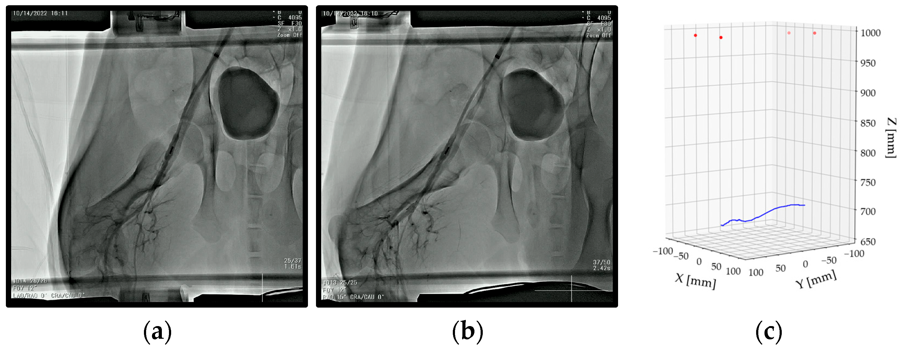
2.5. Three-Dimensional Centerline Reconstruction of a Vascular Map Utilizing TMPR

In Section 2.3 and Section 2.4, we assumed a clear correspondence of points between two images. However, this correspondence is not clear for the path where the pixel points are continuously connected and close to each other. To solve this problem and reconstruct a vascular map, Liao [19] defined an energy function as the objective function which is designed to achieve accurate vessel centerline reconstruction while maintaining a smooth vascular structure. The best 3D coordinates were estimated by minimizing this energy function, as shown in (16), even if the correspondence relationship was not clear:

$$E\left(\mathbb{Z}\right)=\sum _{r\in \mathbb{R}}{\mathcal{D}}_r\left(Z_r\right)+\beta \sum _{r\in \mathbb{R}}\sum _{s\in \mathbb{S}}{V}_{r,s}\left(Z_r,Z_s\right)$$

(16)

where r represents a pixel point on 2D blood vessel centerline extracted from the I_ref, and s denotes a neighborhood point of r. ℝ and 𝕊 denote the set of r and s, respectively. $𝒟$_r(Z_r) is the average pixel distance of each point r, which is a distance between a projected pixel point and the nearest point on the centerline in I_corr. V_r,s(Z_r,Z_s) is the smoothness term representing the difference in Z coordinates from neighborhood points, and β is the coefficient of the sum of smoothness term. ℤ denotes a set of Z coordinates for all r. To find the optimal solution of E(ℤ), Liao utilized the α-expansion method [22] to minimize the energy function by changing the Z coordinate of each r for every equal interval. The accuracy and computation cost of the α-expansion method are affected by the initial Z coordinate because this method iteratively searches the optimal Z coordinate from the initial Z coordinate to minimize the energy function. Liao selected initial Z coordinates of each point randomly or in fixed order. However, we can effectively determine the initial Z coordinate utilizing the proposed TMPR.

Subsequently, the overall process of reconstructing the vascular map using TMPR is described and illustrated in Figure 4. The X-ray images at V_ref and V_corr are denoted as I_ref and I_corr, respectively. The points located along the vascular centerline in I_ref and I_corr are defined as r_ref and r_corr, respectively, with the sets of these points represented as ℝ_ref and ℝ_corr. The points r_ref and r_corr are indexed sequentially along the vascular direction, and the number of points included in ℝ_ref and ℝ_corr may not be equal, depending on the range of the blood vessel captured in each image.

In Figure 4a,b, indices are assigned from the upper-left to the lower-right of I_ref and I_corr, following the vascular direction. Figure 4a,b represents ℝ_ref and ℝ_corr, respectively. After indexing ℝ_ref and ℝ_corr, the line l_proj is calculated for each r_ref using (11) from Section 2.3. Among the points r_ref in Figure 4c, those whose l_proj intersect the line connecting all r_corr points in ℝ_corr at one point, as shown in Figure 4d, are identified. The point r_ref with the smallest index among them is designated as r_ref(k). The point r_corr closest to l_proj of r_ref(k), denoted as r_corr(t), is then assigned as p_opt corresponding to r_ref(k). Once p_opt for r_ref(k) is determined as r_corr(t), the points p_opt corresponding to the remaining points can be assigned using the following algorithm. First, l_proj is calculated for r_ref(k + 1), and the candidate points in ℝ_corr that satisfy the distance constraint are identified. The distance constraint ensures that the distance between l_proj and a given r_corr point does not exceed d_const. Depending on the vessel geometry, there may be one, multiple, or no r_corr points, as illustrated in Figure 4e,f, Figure 4g,h, and Figure 4i,j, respectively.

Figure 4e,f depicts the case where only one point of r_corr meets the distance constraint. If the index of this r_corr point, r_corr(t + 1), is greater than t (the index of the previously assigned p_opt), then r_corr(t + 1) is designated as p_opt for r_ref(k + 1). However, if the index of r_corr(t + 1) is less than or equal to t, p_opt corresponding to r_ref(k + 1) cannot be determined. Figure 4g,h illustrates the case where multiple points of r_corr satisfy the distance constraint. The points of r_corr that satisfy the distance constraint with l_proj of r_ref(k + 2) are r_corr(t + 2), r_corr(t + 3), and r_corr(t + 4). The point with the smallest index greater than the previously assigned indices (t, t + 1) is selected as p_opt, which is r_corr(t + 2). Likewise, if the index of r_corr(t + 2) is less than or equal to t or t + 1, p_opt corresponding to r_ref(k + 2) cannot be determined. Similarly, if no r_corr points satisfy the distance constraint, as shown in Figure 4i,j, p_opt cannot be assigned. After assigning p_opt to all r_ref points, the points r_ref which have p_opt are classified as Group 1 and the points r_ref which do not have p_opt are classified as Group 2. The points p_opt for Group 2 are assigned using the interpolation method. Figure 4i,j illustrates the process for determining p_opt for r_ref(k + 6) of Group 2 due to the absence of r_corr satisfying the distance constraint. r_ref(k + 5) and r_ref(k + 7) belong to Group 1, and if their p_opt are r_corr(t + 6) and r_corr(t + 7), respectively, then p_opt for r_ref(k + 6) is selected from the point lying on the line connecting r_corr(t + 6) and r_corr(t + 7) in such a way that the ratio of the number of pixels between r_ref(k + 5) and r_ref(k + 6) (a₁) to the number of pixels between r_ref(k + 6) and r_ref(k + 7) (a₂) is equal to the ratio of the number of pixels between r_corr(t + 6) and p_opt (a₃) to the number of pixels between r_corr(t + 7) and p_opt (a₄).

After determining the p_opt for every r_ref, initial $Z$ coordinates can be calculated using (9) and (10). Finally, through the α-expansion method that searches the optimal Z with the proposed initial Z coordinates, an energy function can be minimized and the 3D coordinates of a blood vessel centerline can be calculated. In all iterations, TMPR was used to transform between the 3D coordinate system of the C-arm and the 2D coordinate system of the X-ray image.

3. Experimental Results

We developed a program using LabVIEW 2020 (National Instruments, Austin, TX, USA) to realize the proposed TMPR, for the identification of the MNS workspace, and for the 3D reconstruction of a vascular map. We validated the results by performing an in vitro experiment of an MNS mock-up and a vascular jig and an in vivo experiment in which an MMR was remotely operated in the SFA of a mini pig.

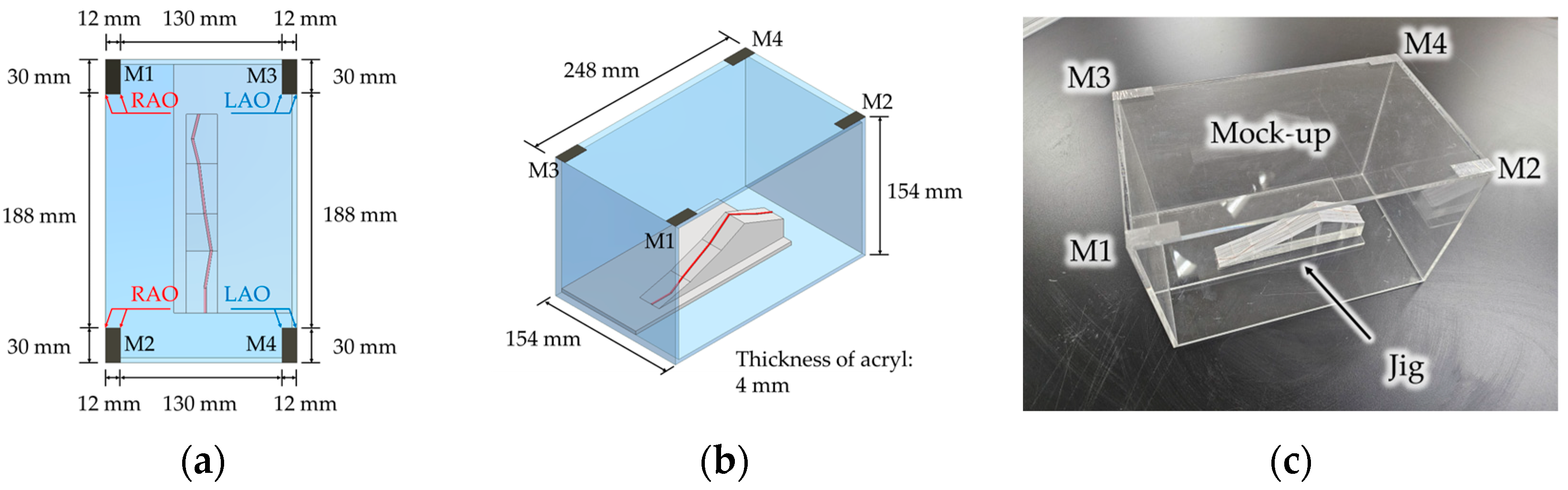
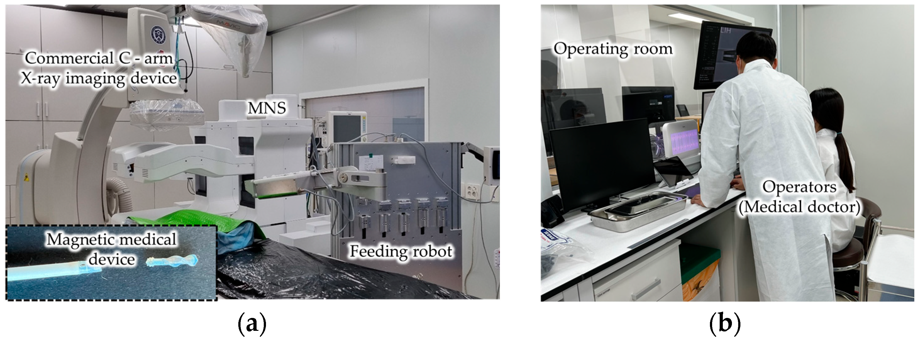
3.1. In Vitro Experiment

Figure 5 shows an in vitro experiment where a mock-up simulating an MNS workspace was designed as a rectangular acrylic box, and a jig simulating a simplified 3D centerline of a blood vessel was designed with a copper wire. At the four corners on the top of the mock-up, we attached four radiopaque tapes (M₁, M₂, M₃, and M₄), whose width and height were 12 mm and 30 mm, respectively. The distance between M₁ and M₃ or M₂ and M₄ was 130 mm, and the distance between M₁ and M₂ or M₃ and M₄ was 188 mm. During the experiments, the inner four corners of two markers (M₁ and M₂ for RAO rotation and M₃ and M₄ for LAO rotation) on one side were utilized as corresponding points, as shown in Figure 5a. Also, the width of each tape (12 mm) and the distance from a marker to the opposite marker (188 mm) were utilized as the distance constraints described in Section 2.4. In the jig, the shape of the 3D centerline was designed as a straight line on the surface of the jig to accurately obtain the actual coordinates. The actual coordinates of the 3D centerline and the four corners in the C_ref were determined from the design values and from measurements using a laser sensor (OD1000, SICK AG, Waldkirch, Germany). The C-arm in this experiment was an Artis Zee Biplane rf-1000-125 (Siemens Healthineers, Forchheim, Germany), a biplane C-arm, of which we utilized only a single C-arm. The resolution of the rotation angle displayed on the control program was 1°. The output image size was 1024 × 1024 pixels, and each pixel had the same height and width. The actual length of 1 pixel in the image was 0.36 mm when the SID was 1200 mm. The sign of the rotation angle was set as positive for the RAO and CAUD directions and negative for the LAO and CRAN directions, considering the signs of the X and Y axes in C_ref. An anterior–posterior (AP) view was captured as a reference view (V_ref), and the other 20 views were captured as corresponding views (V_corr) under the 20 combinations of ±10° and ±15° in the RAO/LAO direction (θ_disp) and 0°, ±5°, and ±10° in the CAUD/CRAN direction (φ_disp).

First, we calculated the relative rotation angle of the C-arm between the two views and the 3D coordinates of the four corners in C_ref, utilizing the proposed method. We placed the mock-up and the jig on the patient bed, and we captured I_ref and I_corr by rotating the C-arm in the order of RAO/LAO(θ) and CAUD/CRAN(φ). The 2D coordinates of the four corners in each image (p_ref, p_corr) were detected using the vision assistant module of LabVIEW. Then, for every relative rotation angle within the range defined by (13), we calculated the d(l_proj, p_corr) of the four corresponding points and the distances between the 3D coordinates of corresponding points by changing the rotation angle by 0.1°. The d_const in (13) was set as two pixels, and the set of ${\mathbb{A}}_{\theta ,\phi }^{*}$ that satisfies (13) was determined. Then, the ${\mathbb{A}}_{\theta ,\phi }^{opt}$ with the minimum error of (14) was determined among the set of ${\mathbb{A}}_{\theta ,\phi }^{*}$. Although there were multiple values of ${\mathbb{A}}_{\theta ,\phi }^{*}$ that satisfy (13), ${\mathbb{A}}_{\theta ,\phi }^{opt}$ can be uniquely determined using the distances between the calculated 3D coordinates of the corresponding points.

After the estimation of the relative rotation angle between two views (V_ref, V_corr), we conducted a 3D centerline reconstruction of the simulated blood vessel (copper wire) in the jig utilizing the proposed method in Section 2.3. And, we analyzed the accuracy of the 3D centerline reconstruction, as shown in

Table 1. The 2D and 3D errors between the calculated and actual coordinates for the centerline of a jig.

${\mathit{\theta }}_{\mathit{d}\mathit{i}\mathit{s}\mathit{p}}$ [°]	${\mathit{\phi }}_{\mathit{d}\mathit{i}\mathit{s}\mathit{p}}$ [°]	2D Errors [mm]			3D Errors
		Max.	Min.	Mean	Max.	Min.	Mean
−15	−10	0.266	0.003	0.101	1.883	0.022	0.669
	−5	0.231	0.001	0.097	1.088	0.004	0.438
	0	0.197	0.001	0.073	0.881	0.000	0.357
	5	0.249	0.001	0.113	0.879	0.007	0.279
	10	0.312	0.003	0.119	1.189	0.010	0.336
−10	−10	0.305	0.001	0.089	1.552	0.012	0.521
	−5	0.250	0.002	0.089	2.079	0.007	0.528
	0	0.181	0.006	0.125	2.479	0.048	0.943
	5	0.240	0.003	0.093	1.516	0.004	0.336
	10	0.308	0.001	0.103	1.162	0.004	0.368
10	−10	0.401	0.003	0.099	1.533	0.007	0.447
	−5	0.341	0.003	0.098	3.203	0.007	0.781
	0	0.190	0.001	0.103	2.442	0.038	0.946
	5	0.456	0.005	0.101	1.589	0.007	0.409
	10	0.782	0.003	0.105	2.617	0.036	1.168
15	−10	0.318	0.001	0.103	1.821	0.016	0.670
	−5	0.292	0.001	0.101	1.826	0.034	0.770
	0	0.193	0.003	0.089	1.642	0.217	0.911
	5	0.263	0.005	0.111	1.707	0.015	0.574
	10	0.311	0.002	0.118	2.133	0.016	0.870

. First, we analyzed the 2D errors of the reconstructed vascular map. The 2D position errors mean the distances between the final p_opt that corresponds to the 596-pixel points of the 2D centerline and the projected pixel points of the actual coordinates of the 3D centerline for each I_corr. Second, we analyzed the 3D position errors of the reconstructed vascular map. The 3D errors mean the distances between the calculated 3D coordinates of every pixel point along the centerline and the actual 3D coordinates of a jig. After calculating the 2D and 3D errors, we calculated the maximum, minimum, and mean of them. According to the results, the 3D coordinates of the centerline pixel points indicated on the jig were calculated with the mean 2D errors between 0.073 mm and 0.125 mm and the mean 3D errors between 0.279 mm and 1.168 mm. The calculated 3D errors were within the diameter range of the femoral artery (8.2–9.8 mm) [23]. In conclusion, the overall pixel points of the centerline were accurately calculated considering the 2D and 3D position errors.

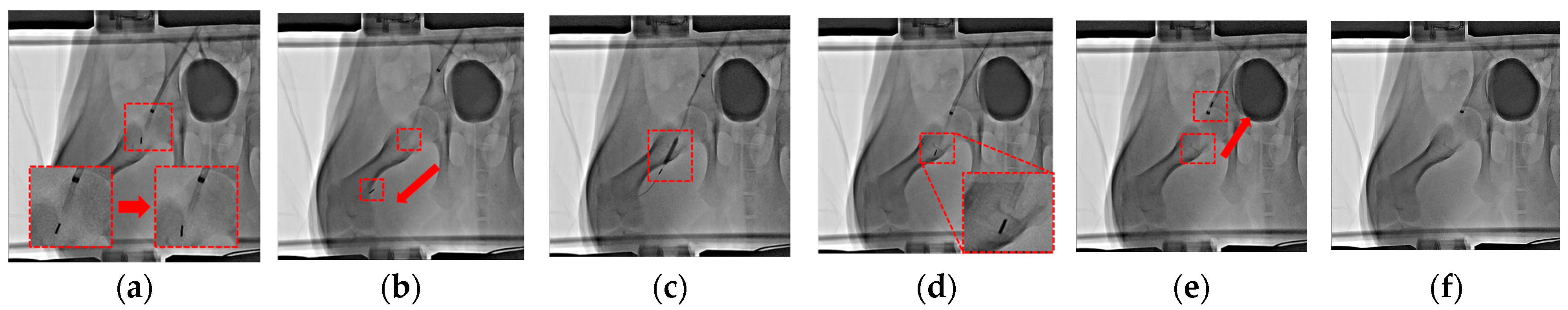
3.2. In Vivo Experiment

This section introduces the result of the reconstruction of a 3D coordinate system of a C-arm and a vascular map of a mini pig’s SFA for the operation of an MMR controlled by an MNS using two X-ray images and four corners of the MNS. We also controlled the magnetic field to operate the MMR along the SFA. This animal experiment was conducted with the approval of the Animal Experiment Ethics Committee of Yonsei University Medical Center (Approval Number: CPEC-IACUC-22-1008) and conformed to the Animal Protection Act (Law No. 16544, enacted on 27 August 2019) and the Laboratory Animal Act (Law No. 15944, enacted on 12 March 2019). Figure 6 shows the experimental setup. The experimental space is divided into an operating room where the procedure is conducted and a control room where a medical doctor can control the procedure remotely to avoid the radiation hazard. The operating room is equipped with a feeding robot, an MNS, and a commercial C-arm. The feeding robot consists of a feeding part to insert a delivery catheter with an untethered micro robot and a guidewire into the vessel, and a syringe part to inject contrast agent and drug into the vessel. The MNS used in this experiment was a RAMAN system (RAMAN-01, Intermag Inc., Seoul, Republic of Korea) [7]. To calculate the relative rotation angle between the two views, we utilized four corners of the RAMAN system’s upper electromagnets as the corresponding points, as shown in Figure 7. For the two electromagnets connected by the same back yoke, the distance between the inner corners is 55.0 mm and the distance between the outer corners is 69.5 mm, as shown in Figure 7a. In addition, the distance between the two electromagnets located on opposite sides was 200.0 mm, as shown in Figure 7b. We set the four corresponding points from the four inner or four outer corners of the two electromagnets, which are more clearly captured in the X-ray image. The selected corresponding points indicate the position of the electromagnet and, therefore, can be used to determine the 3D coordinate system of the MNS workspace.

The commercial C-arm used in the experiment was an INFX-8000V (Canon Medical Systems Corporation, Otawara, Japan). The P_iso was located at a point 696.0 mm away from the source of the C-arm, and the actual length of 1 pixel was 0.262 mm when the SID was at a maximum of 1250 mm. The rotation angle of the C-arm was displayed through the control program at a resolution of 1°. During the procedure, we set the SID to the maximum configuration (1250 mm), and we selected V_ref as the AP view and V_corr as the RAO 15° view (𝔸_15°,0°) for the right SFA and the LAO 15° view (𝔸_−15°,0°) for the left SFA to avoid collision between the C-arm and the RAMAN system. The MMR utilized in this experiment was a separable and recombinable magnetic robot (SRMR) [24] that can be separated and recombined with a delivery catheter, and the mini pig was a Yucatan miniature.

Before the main procedure, the SRMR attached to the delivery catheter was inserted near the target lesion by the feeding device. Then, the C-arm was rotated by RAO 15° (𝔸_15°,0°) or LAO 15 ° (𝔸_−15°,0°), and a contrast agent was injected into the vessels to capture I_corr. The C-arm was then rotated to the AP view, and a contrast agent was injected again to capture I_ref. The pixel coordinates of the four corners were detected using the vision assistant module of LabVIEW from the captured I_ref and I_corr. Then, the relative rotational angles between the two views (${\mathbb{A}}_{\theta ,\phi }^{opt}$) were calculated utilizing the proposed method in Section 2.4, and were ${\mathbb{A}}_{15°,0°}^{opt}=\left(16.3°,-0.7°\right)$ and ${\mathbb{A}}_{-15°,0°}^{opt}=\left(-16.5°,0°\right)$, and the average distance errors between the four corresponding points were 0.341 mm and 0.324 mm, respectively. Also, 3D coordinates of the corresponding points were calculated in C_ref. Subsequently, the contour of the vessel where an SRMR will be operated was manually selected from I_ref and I_corr, and the centerlines of the blood vessel were enhanced by skeletonization in I_ref and I_corr. Finally, the 3D coordinates of a blood vessel’s centerline were calculated in the C_ref using the calculated relative rotation angles and the method proposed in Section 2.5 and were then transformed into the 3D coordinate system of the MNS workspace by considering the calculated coordinates of the four corresponding points. Once two 2D X-ray images are ready, it takes 18.7 s in a computer with an Intel Core i7-11700KF CPU (Intel, Santa Clara, CA, USA), 32 GB DDR4 RAM, and an NVIDIA GeForce GTX 760 GPU (NVIDIA, Santa Clara, CA, USA) to compute the 3D coordinates of 596 points.

Figure 8 shows the X-ray images of right SFA of the mini pig and the 3D plot of corresponding points and the centerline of the SFA calculated using the method proposed in Section 2.5. The C-arm was maintained in the AP view during the rest of the procedure. To control the SRMR inserted into the vessel, the current I_opt needs to be calculated and supplied to the electromagnets of the RAMAN system to generate the required magnetic field (B) and magnetic force (F). The RAMAN system generates a nonuniform magnetic field within the workspace and controls the magnetic field depending on the position P in the 3D coordinate system of MNS workspace. When the SRMR is positioned at a specific location P, the magnetic field and force can be calculated using the following equation [25]:

$$\left[\begin{array}{c}\mathbf{B}\left(\mathbf{P}\right)\\ \mathbf{F}\left(\mathbf{m},\mathbf{P}\right)\end{array}\right]={\mathbf{A}}_{\mathbf{B},\mathbf{F}}{\mathbf{I}}_{\mathrm{o}\mathrm{p}\mathrm{t}}={\mathbf{A}}_{\mathbf{B},\mathbf{F}}\left(\mathbf{m},\mathbf{P}\right)\left({\mathbf{I}}_{\mathbf{B}}+{\mathbf{I}}_{\mathbf{F}}+{\mathrm{C}}_1·{\mathbf{I}}_{\mathrm{n}\mathrm{u}\mathrm{l}\mathrm{l},1}+{\mathrm{C}}_2·{\mathbf{I}}_{\mathrm{n}\mathrm{u}\mathrm{l}\mathrm{l},2}\right)$$

(17)

where m, P, A_B,F, I_B, I_F, I_null,1, I_null,2, C₁, and C₂ represent the magnetic moment of the permanent magnet included in the SRMR, the 3D coordinates of permanent magnet to generate the magnetic field, the actuation matrix of the RAMAN system, the particular solution of currents required to generate the desired magnetic field and forces, the null spaces of the current solutions, and the coefficients of the null space. A_B,F was a 6 × 8 matrix determined by the magnetic moments of the permanent magnet and the position of the SRMR in the 3D coordinate system of the MNS workspace. After the currents needed to generate the required magnetic field at the centerline of the blood vessel are calculated, the position of the SRMR inserted into the blood vessel was recognized from I_ref in real time, and the required magnetic field was generated accordingly.

The procedure was successfully performed, as shown in Figure 9, through the following steps: insertion of the SRMR and delivery catheter into the blood vessel, separation of the SRMR and delivery catheter, forward movement of the SRMR, balloon inflation after the thrombus tunneling, balloon deflation, backward movement of the SRMR, recombination of the SRMR to the delivery catheter, and retrieval of the delivery catheter with the SRMR from the mini pig.

4. Conclusions

We proposed a TMPR that reconstructs 3D coordinates and a vascular map to effectively control an MMR by an MNS. The proposed TMPR transforms two 2D X-ray pixel images into 3D real-world coordinates in the coordinate system of a C-arm. We calculated the relative rotation angle of the C-arm, considering its rotational precision error, by utilizing the TMPR. Also, the TMPR was utilized to reconstruct the vascular map. The reconstructed vascular map is in the 3D coordinate system of the C-arm, and it can be transformed into the 3D coordinate system of the MNS workspace to generate the desired direction and magnitude of the magnetic flux density along the vascular path. The proposed methods were validated through in vitro experiments with a mock-up of an MNS and a vascular jig. Finally, the proposed method was applied to in vivo experiments where the MMR was inserted into the SFA of a mini pig and the motion was precisely controlled remotely by the MNS. This research will enable more precise and effective control of MMRs in various medical procedures utilizing the MNS, and it confirms that the proposed method can enhance the compatibility between commercial C-arm X-ray devices and MNSs in a constrained environment where the maximum angular difference between the two X-ray images is approximately 15°. In future work, it will be necessary to develop a model that reflects vascular changes caused by stenosis or spasm, and to validate the proposed method in complex vascular structures such as cerebral vessels.

References

1. Shamsudhin, N.; Zverev, V.I.; Keller, H.; Pane, S.; Egolf, P.W.; Nelson, B.J.; Tishin, A.M. Magnetically guided capsule endoscopy. Med. Phys. 2017, 44, 91–111. [Google Scholar] [CrossRef] [PubMed]
2. Lee, W.; Nam, J.; Kim, J.; Jung, E.; Kim, N.; Jang, G. Steering, tunneling, and stent delivery of a multifunctional magnetic catheter robot to treat occlusive vascular disease. IEEE Trans. Ind. Electron. 2020, 68, 391–400. [Google Scholar] [CrossRef]
3. Jung, E.; Nam, J.; Lee, W.; Kim, J.; Jang, G. Crawling magnetic robot to perform a biopsy in tubular environments by controlling a magnetic field. Appl. Sci. 2021, 11, 5292. [Google Scholar] [CrossRef]
4. Dodampegama, S.; Mudugamuwa, A.; Konara, M.; Perera, N.; De Silva, D.; Roshan, U.; Tamura, H. A review on the motion of magnetically actuated bio-inspired microrobots. Appl. Sci. 2022, 12, 11542. [Google Scholar] [CrossRef]
5. Jeon, S.; Jang, G.; Choi, H.; Park, S. Magnetic navigation system with gradient and uniform saddle coils for the wireless manipulation of micro-robots in human blood vessels. IEEE Trans. Magn. 2010, 46, 1943–1946. [Google Scholar] [CrossRef]
6. Kummer, M.P.; Abbott, J.J.; Kratochvil, B.E.; Borer, R.; Sengul, A.; Nelson, B.J. OctoMag: An electromagnetic system for 5-DOF wireless micromanipulation. IEEE Trans. Robot. 2010, 26, 1006–1017. [Google Scholar] [CrossRef]
7. Lee, W.; Jung, E.; Kim, N.; Lee, D.; Kim, S.; Lee, Y.; Jang, G. Robotically adjustable magnetic navigation system for medical magnetic milli/microrobots. IEEE/ASME Trans. Mechatron. 2024, 29, 3949–3959. [Google Scholar] [CrossRef]
8. Oulmas, A.; Andreff, N.; Régnier, S. Closed-loop 3d path following of scaled-up helical microswimmers. In Proceedings of the 2016 IEEE International Conference on Robotics and Automation, Stockholm, Sweden, 16–21 May 2016. [Google Scholar]
9. Wu, X.; Liu, J.; Huang, C.; Su, M.; Xu, T. 3-D path following of helical microswimmers with an adaptive orientation compensation model. IEEE Trans. Autom. Sci. Eng. 2019, 17, 823–832. [Google Scholar] [CrossRef]
10. Zhao, H.; Leclerc, J.; Feucht, M.; Bailey, O.; Becker, A.T. 3d path-following using mrac on a millimeter-scale spiral-type magnetic robot. IEEE Robot. Autom. Lett. 2020, 5, 1564–1571. [Google Scholar] [CrossRef]
11. Xu, T.; Guan, Y.; Liu, J.; Wu, X. Image-based visual servoing of helical microswimmers for planar path following. IEEE Trans. Autom. Sci. Eng. 2019, 17, 325–333. [Google Scholar] [CrossRef]
12. Nguyen, P.B.; Park, J.O.; Park, S.; Ko, S.Y. Medical micro-robot navigation using image processing-blood vessel extraction and X-ray calibration. In Proceedings of the 2016 6th IEEE International Conference on Biomedical Robotics and Biomechatronics (BioRob), Singapore, 26–29 June 2016; pp. 365–370. [Google Scholar]
13. Movassaghi, B.; Rasche, V.; Grass, M.; Viergever, M.A.; Niessen, W.J. A quantitative analysis of 3-D coronary modeling from two or more projection images. IEEE Trans. Med. Imaging 2004, 23, 1517–1531. [Google Scholar] [CrossRef] [PubMed]
14. Yang, J.; Wang, Y.; Liu, Y.; Tang, S.; Chen, W. Novel approach for 3-D reconstruction of coronary arteries from two uncalibrated angiographic images. IEEE Trans. Image Process. 2009, 18, 1563–1572. [Google Scholar] [CrossRef] [PubMed]
15. Fu, Z.; Fu, Z.; Gong, Z.; Feng, X.; Gu, H.; Xie, R.; Fei, J. Optimization for 3D reconstruction of coronary artery tree by two-stage Levenberg-Marquardt algorithm. In Proceedings of the 2021 27th International Conference on Mechatronics and Machine Vision in Practice, Shanghai, China, 26–28 November 2021. [Google Scholar]
16. Chen, S.J.; Carroll, J.D. 3-D reconstruction of coronary arterial tree to optimize angiographic visualization. IEEE Trans. Med. Imaging 2000, 19, 318–336. [Google Scholar] [CrossRef]
17. Banerjee, A.; Galassi, F.; Zacur, E.; De Maria, G.L.; Choudhury, R.P.; Grau, V. Point-cloud method for automated 3D coronary tree reconstruction from multiple non-simultaneous angiographic projections. IEEE Trans. Med. Imaging 2019, 39, 1278–1290. [Google Scholar] [CrossRef]
18. Blondel, C.; Malandain, G.; Vaillant, R.; Ayache, N. Reconstruction of coronary arteries from a single rotational X-ray projection sequence. IEEE Trans. Med. Imaging 2006, 25, 653–663. [Google Scholar] [CrossRef] [PubMed]
19. Liao, R.; Luc, D.; Sun, Y.; Kirchberg, K. 3-D reconstruction of the coronary artery tree from multiple views of a rotational X-ray angiography. Int. J. Cardiovasc. Imaging 2010, 26, 733–749. [Google Scholar] [CrossRef]
20. Cesar, A.; Grkman, M.; Medic, M. Magnification error in radiographs of cervical spine in lateral projection. Med. Imaging Radiother. J. 2020, 37, 15–19. [Google Scholar] [CrossRef]
21. Çimen, S.; Gooya, A.; Grass, M.; Frangi, A.F. Reconstruction of coronary arteries from X-ray angiography: A review. Med. Image Anal. 2016, 32, 46–68. [Google Scholar] [CrossRef]
22. Boykov, Y.; Veksler, O.; Zabih, R. Fast approximate energy minimization via graph cuts. IEEE Trans. Pattern Anal. Mach. Intell. 2001, 23, 1222–1239. [Google Scholar] [CrossRef]
23. Sandgren, T.; Sonesson, B.; Ahlgren, Å.R.; Länne, T. The diameter of the common femoral artery in healthy human: Influence of sex, age, and body size. J. Vasc. Surg. 1999, 29, 503–510. [Google Scholar] [CrossRef]
24. Sa, J.; Park, J.; Jung, E.; Kim, N.; Lee, D.; Bae, S.; Jang, G. Separable and recombinable magnetic robot for robotic endovascular intervention. IEEE Robot. Autom. Lett. 2023, 8, 1881–1888. [Google Scholar] [CrossRef]
25. Lee, S.; Kim, N.; Kwon, J.; Jang, G. Identification of the position of a tethered delivery catheter to retrieve an untethered magnetic robot in a vascular environment. Micromachines 2023, 14, 724. [Google Scholar] [CrossRef] [PubMed]
Figure 1. (a) Diagram of the source, detector, SID, SOD, image size, and object size; and (b) coordinate system of the C-arm and X-ray image.
Applsci 15 06089 g001
Figure 2. (a) Initial 3D coordinate system of the C-arm and a point Pinit in the C-arm workspace; (b) rotating the C-arm by δ when a point Pinit is fixed; and (c) rotating Pinit by −δ when the C-arm is fixed.
Applsci 15 06089 g002
Figure 3. (a) pref and p0 in Iref; (b) Cref and Pinit; (c) Crot and Prot; and (d) pcorr, lproj, and popt in Icorr.
Applsci 15 06089 g003
Figure 4. (a) Coordinate axes of Iref, ℝref, rref, and the index of rref; (b) coordinate axes of Icorr, ℝcorr, rcorr, and the index of rcorr; (c) rref(k) in Iref; (d) lproj of rref(k) and rcorr(t) selected as popt of rref(k); (e) rref(k + 1) in Iref; (f) lproj of rref(k + 1) and rcorr(t + 1) selected as popt of rref(k + 1); (g) rref(k + 2) in Iref; (h) lproj of rref(k + 2) and candidate points rcorr(t + 2), rcorr(t + 3), and rcorr(t + 4) for popt selection of rref(k + 2); (i) rref(k + 5), rref(k + 6), and rref(k + 7) in Iref, where a1 represents the number of pixels between rref(k + 5) and rref(k + 6), and a2 represents the number of pixels between rref(k + 6) and rref(k + 7); (j) rcorr(t + 6), rcorr(t + 7), lproj of rref(k + 6), and popt of rref(k + 6) in Icorr, where a3 represents the number of pixels between popt of rref(k + 6) and rcorr(t + 6), and a4 represents the number of pixels between popt of rref(k + 6) and rcorr(t + 7).
Applsci 15 06089 g004
Figure 5. A mock-up and a jig that simulates an MNS workspace and a blood vessel for an in vitro experiment. (a) Top view; (b) side view; and (c) photograph.
Applsci 15 06089 g005
Figure 6. Experimental environments for the in vivo experiment. (a) Operating room; and (b) control room.
Applsci 15 06089 g006
Figure 7. Corners of the upper electromagnets of the RAMAN system utilized as corresponding points: (a) side view; and (b) top view.
Applsci 15 06089 g007
Figure 8. (a) Iref (AP) of the right SFA; (b) Icorr (RAO 15°) of the right SFA; and (c) a 3D plot of corresponding points (red) and the centerline of the right SFA (blue) calculated using the proposed reconstruction method of a vascular map.
Applsci 15 06089 g008
Figure 9. In vitro experiment along the right SFA using the RAMAN system, feeding robot, and SRMR after generating a 3D blood vessel map. (a) Separation; (b) movement forward; (c) balloon inflation; (d) movement backward; (e) recombination; and (f) final retrieval.
Applsci 15 06089 g009