Characterization of Driver Dynamic Visual Perception Under Different Road Linearity Conditions

Abstract

Drivers’ visual characteristics have an important impact on traffic safety, but existing studies are mostly limited to single-scene analyses and lack a systematic study on the dynamic changes in drivers’ eye tracking characteristics on different road sections. In this study, 23 drivers were recruited to wear the aSee Glasses eye tracking device and driving tests were conducted on four typical road sections, namely, straight ahead, turning, climbing, and downhill. The average fixation duration, pupil diameter, and the saccade amplitude of the eye tracking were collected, one-way analysis of variance (ANOVA) was used to explore the differences between the different road sections, and a mathematical model of changes in the visual characteristics over time was constructed, based on the fitting of the data. Computerized fitting models of changes over time were also constructed using the Origin 2021 software. The results show that different road sections had significant effects on drivers’ visual tasks: the longest average fixation duration was found in the straight road section, the largest pupil diameter was found in the curved road section, and the highest saccade amplitude was found in the downhill road section, reflecting the influence of the complexity of the driving task on the cognitive load. The fitted model further reveals the dynamic change law of eye tracking indicators over time, providing a quantitative basis for modeling driving behavior and visual tasks. This study provides a theoretical basis and practical reference for the optimal design of advanced driver assistance systems, traffic safety management, and road planning.

1. Introduction

The visual system, as the main sensory system through which drivers acquire road information during driving, plays a decisive role in ensuring driving safety [1,2,3,4,5]. Especially in complex roadway environments such as turns, climbing and downhill sections, and steep curves, drivers face diverse and challenging visual tasks [6]. Different road features have a profound impact on drivers’ visual perception, attention allocation, information processing, and decision-making abilities [7], which in turn affect drivers’ driving behaviors and the incidence of traffic accidents [8].

On straight roadways, drivers are usually able to acquire road information at longer distances with relative ease, thus enabling them to detect potential traffic risks earlier. However, when a vehicle enters a turning or curved roadway, the driver’s visual distance is significantly shortened and the complexity of the visual task increases [9]. Studies have shown that the design of a turning roadway has a significant impact on the driver’s visual task; especially when the curve is sharp or the traffic density is high, the driver needs to pay more attention to the curvature of the roadway and obstacle identification [10]. This visual compression not only affects drivers’ recognition of traffic obstacles but may also give them a tendency to overdrive or underestimate hazards [9,11]. Climbing and downhill segments are equally important in driver visual tasks. Climbing segments usually result in limited visual range for drivers, and the dynamics of a vehicle traveling on an incline require a high level of reaction speed and judgment. In climbing sections, drivers usually underestimate the traffic obstacles ahead, especially in poor road conditions or large gradients, which increases the risk of traffic accidents [12,13]. In contrast, downhill sections pose a greater challenge to drivers’ visual attention and reaction speed. During downhill driving, due to gravity, drivers need to remain alert to ensure safe speeds and monitor the road surface condition and traffic conditions in real time. It has been pointed out that the steepness of a slope affects the driver’s visual assessment of the road environment [14], especially in terms of significant delays in vehicle braking and obstacle-avoidance responses. With the continuous development of advanced driver assistance systems (ADASs) and autonomous driving technologies [15], the assurance of traffic safety has gradually shifted towards automation [16]. Existing driver assistance technologies, such as automatic emergency braking and adaptive cruise control, alleviate the visual pressure of drivers in complex environments to a certain extent [17]. However, these systems still have certain limitations when facing highly complex roadways [18,19]. It is still difficult for current autonomous driving systems to fully simulate the driver’s visual adaptation and judgment process in specific roadway environments [20], and thus the visual ability of human drivers remains one of the key factors in ensuring traffic safety.

In order to gain a deeper understanding of drivers’ visual characteristics in different roadway environments, this study will combine eye tracking, driving simulation experiments, and real road tests to explore drivers’ visual tasks and decision-making patterns in a variety of roadway environments [21], such as straight ahead, turning, climbing, downhill, and sharp curves and steep slopes [22,23]. This study aims to reveal the influence mechanism of different road conditions on drivers’ visual behavior [24] and then provide theoretical basis and data support for road design, traffic safety management, and further development of intelligent driving technology. Through the systematic analysis of drivers’ visual responses in complex road environments [25], this study helps to promote the optimization of traffic safety and the innovative development of intelligent transportation systems.

2. Experimental Design

2.1. Test Road

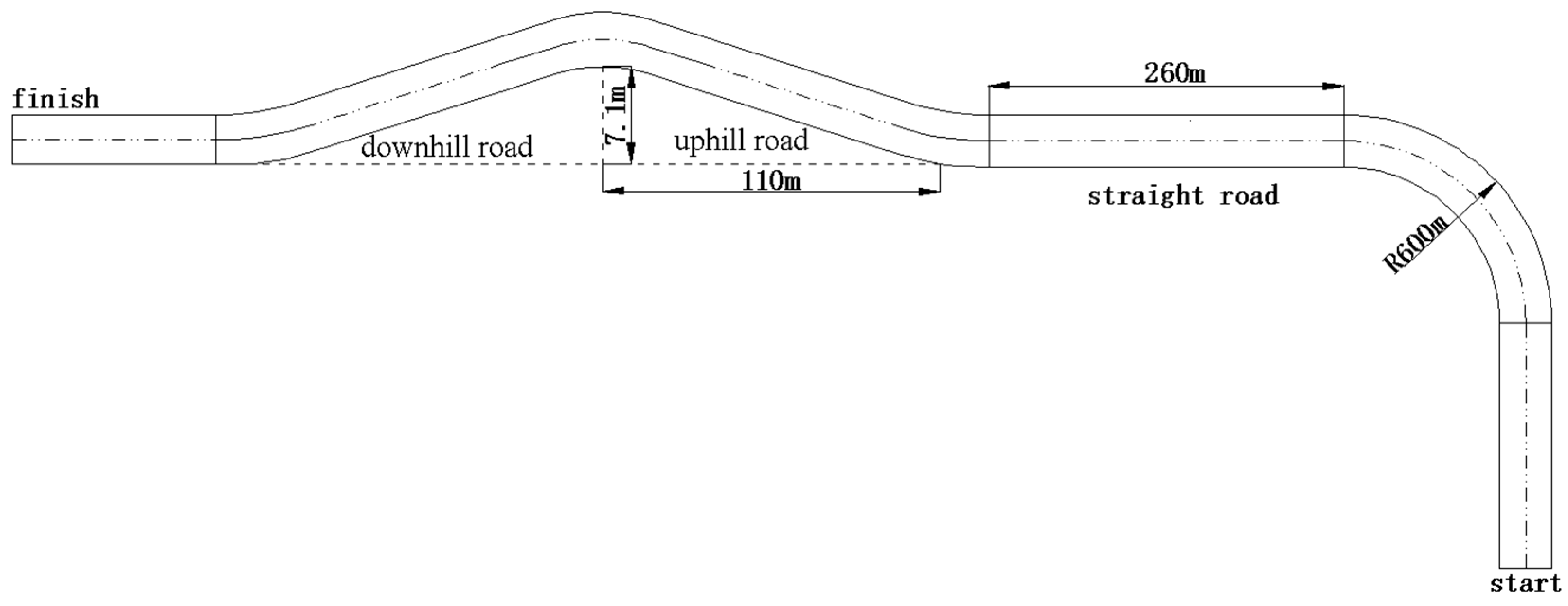
The test road selected was a representative section of a school highway, that is, around the school area, that eases traffic pressure and ensures the traffic safety of students to and from school. In order to comprehensively examine the driver’s visual perception features under different road sections, a circular road was set up, with only the school along the route, which covered the four typical types of roads, a straight line, curves, and an uphill and downhill section. The road section plan is schematically shown in Figure 1. The following factors were considered in the selection of the test roads: the actual traffic conditions of the roads, the complexity of the road sections, the representativeness of the roads, i.e., whether the four typical road types of straight, curved, climbing, and downhill segments were covered, and safety, i.e., this study ensures that the selected roads comply with the traffic safety standards and selected weekends with low traffic flow for the experiments to minimize interference from other vehicles and prevent potential accidents.

The arrangement of the test road was designed according to the following principles: to ensure the typicality and representativeness of different road sections, to minimize traffic interference, and to ensure the safety and controllability of the test process. The length of each road section was controlled to be between two hundred meters and three hundred meters to ensure that drivers could perform driving operations stably and collect sufficient eye tracking data under different road conditions.

2.2. Selection of Test Participants

Since the experiment was conducted in a real road environment and the driving test for each subject needed to include detailed safety and security, equipment installation, and data collection, increasing the sample size would significantly increase the complexity of the experiment and the resources required, thus limiting the sample size. In addition, this experiment was a pilot study to investigate the variability of driver eye movement characteristics under different road conditions and to provide a basis for future extended research. In this paper, 23 drivers were selected as a sample with the aim of collecting sufficient data for preliminary analysis and to provide a basis for a larger study in the future. Twenty-three drivers were selected as experimental subjects for this study, and all subjects met the following criteria: age between 22 to 45, driving experience of no less than 3 years, a valid driver’s license, and no major traffic accidents or violations in the past 3 years. All subjects had normal or corrected visual acuity (≥0.8) and had no eye diseases or diseases that affect vision. The sample consisted of 15 males (65%) and 8 females (35%), with an age distribution of 20–30 years (40%), 31–40 years (43%), and 41–45 years (17%). To control for differences in driving behavior, all subjects’ driving habits conformed to conventional driving patterns and were ensured to be able to perform the experimental tasks successfully through eye tracking operation training and road familiarization prior to the trial.

2.3. Equipment Used in the Test

In this study, an aSee Glasses eye tracking device, a Changan Ford Focus sedan, and an Honor laptop equipped with aSee Studio software v0.3.35.3 were used. aSee Glasses is a spectacle-type eye tracking device developed by “Qixin Yiwei” to record the driver’s eye tracking data and is capable of tracking up to the limit range of human eye rotation and supports tracking of the full field of view angle. With an accuracy of 0.5 degrees and a data acquisition frequency of 120 Hz, it can accurately record a variety of eye movement indicators, such as the number of gazes, gaze duration, pupil diameter, and scanning amplitude with a delay of less than 5 milliseconds and weighs less than 50 g in a dynamic driving scenario [26]. All data were synchronized and stored on a unified platform to ensure the consistency and accuracy of all types of data during analysis, providing comprehensive data support for subsequent eye tracking behavior analysis. However, there are several other commonly used eye tracking software products on the market, such as Tobii Pro Studio, EyeLink Data Viewer, and Pupil Labs. Tobii Pro Studio provides powerful analysis capabilities, but its price is relatively high. EyeLink Data Viewer is suitable for various experimental settings, but the interface is relatively complex; Pupil Labs is an open-source platform with a high degree of customization, but with a steep learning curve. We chose aSee Studio software mainly due to its compatibility with aSee Glasses devices and easy-to-use interface, which was particularly suitable for the needs of this experiment.

2.4. Test Steps

Preparation for the experiment: To ensure the scientific validity and accuracy of the experiment, we checked the weather forecast in advance and chose to conduct the experiment under good weather conditions and suitable light intensity to minimize the effects of weather and time on drivers. All participating vehicles were also thoroughly inspected. First, the mechanical performance of the experimental vehicles was ensured to be in the best condition, including checking the brake system, engine, tire pressure, and so on. Then the aSee Glasses eye tracking device was calibrated at three points—top left, horizontal, and bottom right—with 100% binocular calibration to ensure the accuracy of data collection. All devices were double-checked before testing to avoid any impact on the results due to equipment malfunction. In addition, participants were given a detailed explanation of the experiment, including the purpose, procedure, and points to note, to ensure that they had a full understanding of the experiment, and a short test run was conducted before the start of the experiment to help them familiarize with the roadway and the experimental procedure. In this paper, the experiment was conducted on a weekend with less traffic flow to minimize the interference of external traffic factors, and the subjects were told that they did not need to keep a specific distance from other vehicles and that they should keep their driving speed to 30–50 km/h, i.e., not to exceed the speed limit set by the road.

The process of the experiment: At the starting point of the test section, the subject starts the vehicle to start driving, while the instrumentation collects the data, turning on the data collection 50 m before the driver enters the experimental section, and ending the data collection 50 m after leaving the complex section. The test requires the driver to drive back and forth on the experimental section for two laps, in accordance with his usual driving habits, to ensure the accuracy of the collected data. Before the experiment, we found through the comparison of pre-experimental data that the variability of the data obtained from the collection of different vehicle traveling directions is very small, so it can be stated that the directionality has a low influence on the data.

Data collection: During the experiment, the data collected by the visual tracking device and the camera on the device were transmitted to the connected laptop in real time to ensure the immediacy and accuracy of the data.

End of experiment: At the end of the experiment, all participants underwent a short interview, which was designed to collect subjective feedback from participants on the experimental road conditions and driving experience. Interview questions included the following: (1) Did you find the visual perception task difficult in the different road conditions? (2) Which road sections in the experiment did you find most challenging? (3) Did you experience any discomfort or other factors affecting your driving during the experiment? The summary of the interview content showed that most participants felt more stress in the turning and downhill sections, especially when frequent visual focus adjustments were required, suggesting that their individual variability did not have an impact on the experimental results.

3. Data Analysis

3.1. Delineation of the Fixation Area

Figure 2 illustrates the area of interest (AOI) for driver eye tracking, which is based on the field of view angle to study drivers with a mean horizontal field of view angle of 70° and 10° in the vertical direction [27]. This region represents the driver’s main visual attention area during the experiment, which covers the center of the lane, the far view ahead, and other important road information. Through the division of this region, we were able to analyze the allocation of drivers’ visual attention and further understood the effects of different roadway driving tasks on eye tracking indexes.

3.2. Average Fixation Duration Patterns of Drivers in Different Road Conditions

Average fixation duration is the average of the time the driver’s eyes remain on the target object. This metric is used to assess the ease with which a driver can extract information from the visual environment [28]. Drivers’ average fixation duration on different road sections showed significant differences. As shown in Figure 3, it can be seen that fixation duration was the longest when driving on the straight road section, which was attributed to the fact that the driving task was the simplest, the environment was less dynamic, the driver’s fixation point usually focused on the centerline of the road and the distant road conditions, and the fixation target was stable. In contrast, the task complexity of the turning section was significantly higher, and drivers needed to switch their fixation points quickly to cope with the dynamic environment, so the average fixation duration was the shortest. The task complexity of the climbing section was more complicated than that of the straight road, and drivers mainly focused on the distance to the vehicle in front, the gradient, and the road condition, the fixation targets are relatively concentrated and less changeable, and the fixation duration is between the straight section and the turning section, which was moderately long. The task complexity was highest on the downhill section because the driver needed to switch fixation points frequently to monitor speed, the vehicle in front, and the dynamic road environment, resulting in a fixation duration that was between that of the turn and the climbing section but slightly shorter than that of the climbing section.

To validate the significance of the differences in gaze duration between different road sections, one-way analysis of variance (ANOVA) was used in this study, and the results are shown in

Table 1. One-way ANOVA for Average Fixation Duration.

Source of Difference	SS	df	MS	F	p-Value	F Crit
Between-Group	73.72151	3	24.57384	3.499559	0.019211	2.718785
Between-Group	561.7585	80	7.021982
Sum	635.48	83

. The results of the analysis show that the F-value is 3.499559, which is significantly greater than the critical value F crit = 2.718785, and the p-value is significantly less than 0.05, indicating that the difference in gaze duration between different road sections is statistically significant. This result further confirms the significant effect of different road sections on the average gaze duration of drivers. The statistical analysis using ANOVA in this paper not only verified the differences in gaze duration among straight, turning, climbing, and downhill road sections but also provided a quantitative scientific basis for understanding the allocation of drivers’ visual attention under different road alignments, further supporting the relationship between visual task complexity and cognitive load. Table 2 shows a one-way ANOVA of average pupil diameter.

3.3. Pupil Diameter Patterns of Drivers Under Different Road Conditions

Pupil diameter is the size of the pupil, which is usually used to reflect the physiological and cognitive state of the driver. During driving, changes in pupil diameter can be correlated with the driver’s cognitive load, emotional responses, and the intensity of external stimuli [29]. By graphically analyzing the experimental data from different road sections, the drivers’ pupil diameters showed significant differences in each road section. Figure 4 demonstrates the change of pupil diameter in four kinds of road sections: straight line, turning, climbing, and downhill. From the figure, it can be seen that the driver’s pupil diameter in the turning section was significantly larger than in the other roadway sections, which showed a more obvious dilation trend. This change suggested that the curved roadway had an increased visual burden due to the complexity of the roadway and the driver’s need for higher concentration for visual information processing, thus prompting pupil dilation to improve perceptual ability. In contrast, the pupil diameters of straight sections were relatively small and showed a more stable state. This was due to the fact that straight sections had simple and less changing road morphology, and the driver’s visual task was more homogenous, with a lower need for pupil dilation. The pupil diameters of the climbing and downhill sections increased compared to the straight line, especially in the downhill section, where the driver needed to control the speed and monitor the surrounding dynamic environment more frequently, and the cognitive load was higher, resulting in a more pronounced pupil dilation.

To validate verify the significance of the difference in pupil diameter between different road sections, a one-way analysis of variance (ANOVA) was performed on the pupil diameter data of each road section. The results of the analysis, as shown in Table 2, showed that the differences in pupil diameters between different road sections were statistically significant because F = 3.109245 > F crit = 2.718785, p-value < 0.05. Pupil diameter over time at different road sections was modeled.

Table 2. One-way ANOVA of average pupil diameter.

Source of Difference	SS	df	MS	F	p-Value	F Crit
Between-Group	16.23766	3	5.412553	3.109245	0.030969	2.718785
Between-Group	139.2634	80	1.740793
Sum	155.5011	83

Table 2. One-way ANOVA of average pupil diameter.

Source of Difference	SS	df	MS	F	p-Value	F Crit
Between-Group	16.23766	3	5.412553	3.109245	0.030969	2.718785
Between-Group	139.2634	80	1.740793
Sum	155.5011	83

3.4. Patterns of Saccade Amplitude in Drivers Under Different Road Conditions

Saccadic amplitude refers to the spatial distance traveled by the eye when shifting from one fixation point to the next [29]. This metric was used to measure a driver’s eye tracking amplitude in a visual task and reflected the visual search strategy and task complexity. Saccade amplitude of drivers under different driving conditions was shown in Figure 5. From the figure, it can be observed that the saccade amplitude was the smallest during straight driving. This was primarily due to the simplicity of the driving task and the low environmental dynamics in straight sections. The driver’s fixation point tended to focus on the center of the road or distant targets, resulting in a relatively fixed fixation point and a smaller range of saccadic movement. In contrast, during the turning section, drivers needed to dynamically scan multiple targets, such as the inner and outer edges of the curve as well as road signs. The frequent shifts in fixation, particularly towards distant targets on the outer side of the curve, led to a significant increase in saccade amplitude. In climbing sections, drivers’ fixation was primarily focused on the vehicle ahead and the target at the top of the slope. Due to the relatively static environment and concentrated targets, the range of saccadic movement remains at a moderate level. The downhill section presented the most complex driving task, as drivers need to frequently monitor vehicle speed, obstacles ahead, and distant road targets. The rapid shifts in fixation within a dynamic environment and the broader coverage of visual attention result in the largest saccade amplitude.

The data were further analyzed by using one-way analysis of variance (ANOVA) to analyze the variability of drivers’ average saccade amplitude under different driving sections as shown in

Table 3. One-way ANOVA of mean saccade amplitude.

Source of Difference	SS	df	MS	F	p-Value	F Crit
Between-Group	35147.82	3	11715.94	2.803535	0.04506	2.718785
Between-Group	334319	80	4178.988
Sum	369466.8	83

. According to the results in the table, F = 2.803535 > F crit = 2.718785, p-value < 0.05, and it can be seen that the average saccade amplitude of the drivers under different driving conditions shows significant variability.

4. Model Construction

Based on the results of the variability analysis of the driver’s average fixation duration, pupil diameter, and saccade amplitude under different road conditions in the previous section, it was found that there were significant differences in these indicators under different road conditions. In this section, further in-depth analysis was conducted by segmenting the test data of each tester at 1s intervals and extracting the data of the first 70 s of each tester’s driving on each road section for averaging. Subsequently, the trend of the averaged data was analyzed, and a computer-fitted model of the change of each index over time under different road conditions was established to reveal the dynamic change of drivers’ behavioral characteristics under various road conditions.

For data processing and model construction, the Origin software developed by OriginLab Corporation, version Origin 2021, was used in this study for data analysis and cubic polynomial fitting. The cubic polynomial fitting model was chosen for this study because it fits nonlinear data better and smooths out data fluctuations, which allowed changes in visual features in the time dimension to be accurately described. This method has been widely used in many similar engineering and scientific studies, such as Zhou et al. [30], Tan et al. [31], and Kim et al. [32].

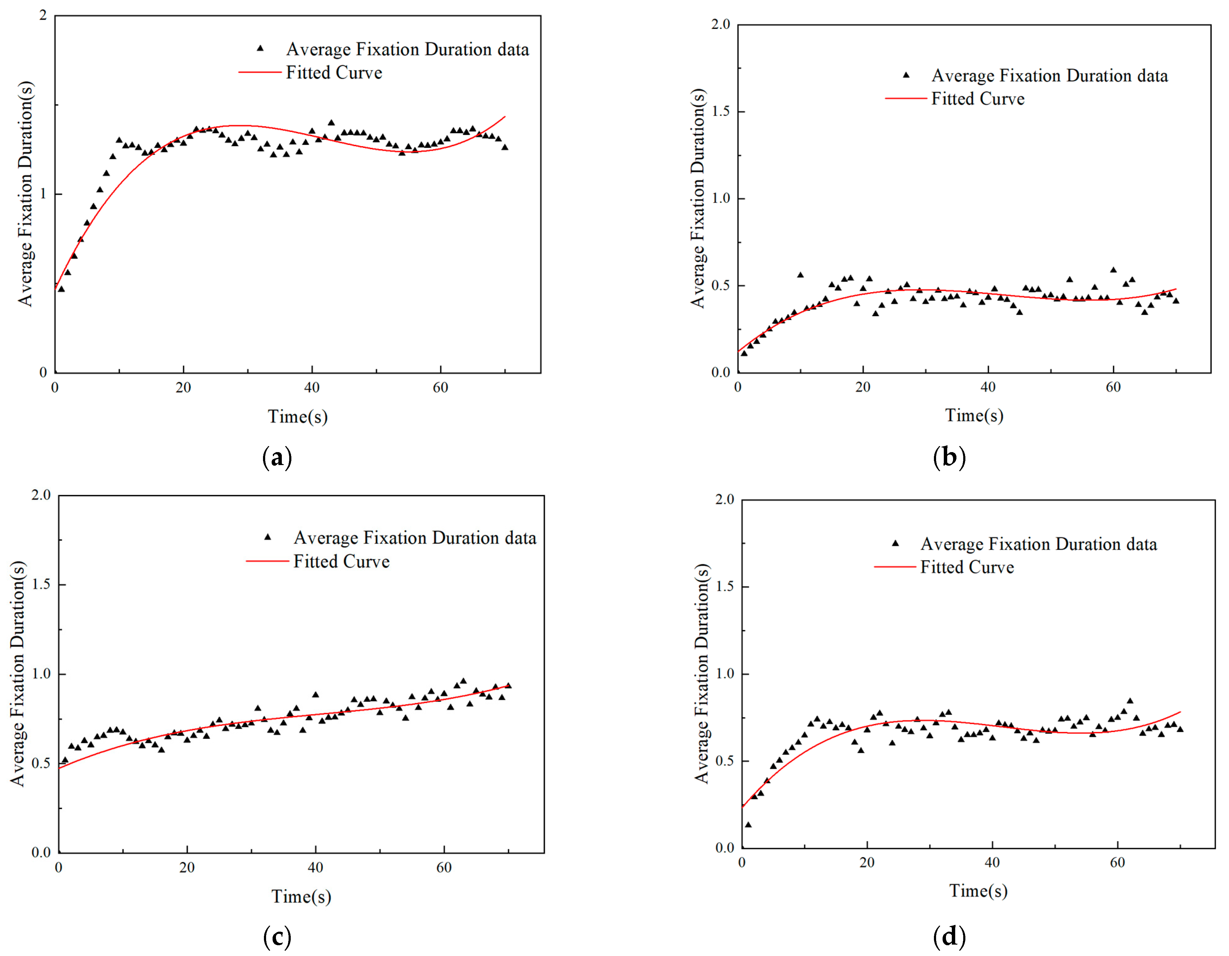
4.1. Modeling of Average Fixation Duration over Time Under Different Road Sections

After importing the processed data into Origin software for cubic polynomial fitting, the trend of average fixation duration over time under different road conditions was calculated and is shown in Figure 6, the fitted model showed excellent fitting effect, and its specific fitting parameters are shown in

Table 4. Model of changes in average fixation duration under different road segments.

Section of Road	Average Fixation Duration Model	${\mathit{R}}^2$
Straight Movement	$y=1.62437{ \times 10}^{-5}{t}^3-0.00204t^2+0.0772t+0.46727$	$0.843$
Turn	$y=6.0543{ \times 10}^{-6}{t}^3-7.72704\times {10}^{-4}{t}^2+0.02957t +0.12151$	$0.701$
Climbing	$y=2.43225{ \times 10}^{-6}{t}^3-2.98094\times {10}^{-4}{t}^2+0.01557t+0.47329$	$0.815$
Downhill	$y=9.01659\times {10}^{-6}{t}^3-0.00112\times {10}^{-4}{t}^2+0.04226t+0.23338$	$0.731$

. The models for average fixation duration under different roadway segments and their fitting results are presented in Table 4. For the straight road section, the fitted model is:

$$\mathrm{y}=1.62437{ \times 10}^{-5}{\mathrm{t}}^3-0.00204{\mathrm{t}}^2+0.0772\mathrm{t}+0.46727$$

(1)

The R² value of this model was 0.843, which indicated that the model can fit the data well, indicating that, in the straight road section, the driver’s cognitive load was low, and the fixation duration showed a smooth increase over time.

For the turning section, the fitted model is

$$\mathrm{y}=6.0543\times {10}^{-6}{\mathrm{t}}^3-7.72704\times {10}^{-4}{\mathrm{t}}^2+0.02957\mathrm{t}+0.12151$$

(2)

The R² value of this model was 0.701, and the relatively low R² value indicates that driver fixation duration fluctuated more in the turning road section, and the fitting effect was not as good as in the straight road section. This is due to the fact that drivers need to adjust their vision frequently when turning and the task complexity was higher, which resulted in increased data volatility.

For the climbing section, the fitting model is:

$$\mathrm{y}=2.43225\times {10}^{-6}{\mathrm{t}}^3-2.98094\times {10}^{-4}{\mathrm{t}}^2+0.01557\mathrm{t}+0.47329$$

(3)

The R² value of this model was 0.815, which indicated that the fitting effect was better for the climbing section, even though there was some data volatility and the driver’s cognitive load was higher at the beginning of the ramp but gradually decreased as he or she adapted to the ramp environment.

For the downhill section, the fitting model is:

$$\mathrm{y}=9.01659\times {10}^{-6}{\mathrm{t}}^3-0.00112\times {10}^{-4}{\mathrm{t}}^2+0.04226\mathrm{t}+0.23338$$

(4)

The model had an R² value of 0.731, and the relatively low R² value indicated that the fixation duration changes were more complicated in the downhill section. Drivers’ cognitive load was higher and fixation duration fluctuates more at the beginning of the downhill section due to the need to control speed and cope with potential hazards, while drivers’ cognitive load gradually decreased as the gradient decreases or the complexity of the environment decreases.

Overall, the model fitted well to the data points under the four road conditions, especially in the straight ahead and climbing segments, showing high prediction accuracy. However, the complexity of the task was greater in the turning and downhill segments, the data points fluctuated more, and the fitted model had some deviations. In addition, the graphs also showed that the average fixation duration gradually increases with the continuation of time for the four road conditions, which may be due to the fatigue caused by the drivers driving for a long time, which reduces the frequency of the fixation behavior and the intensity of the attention allocation.

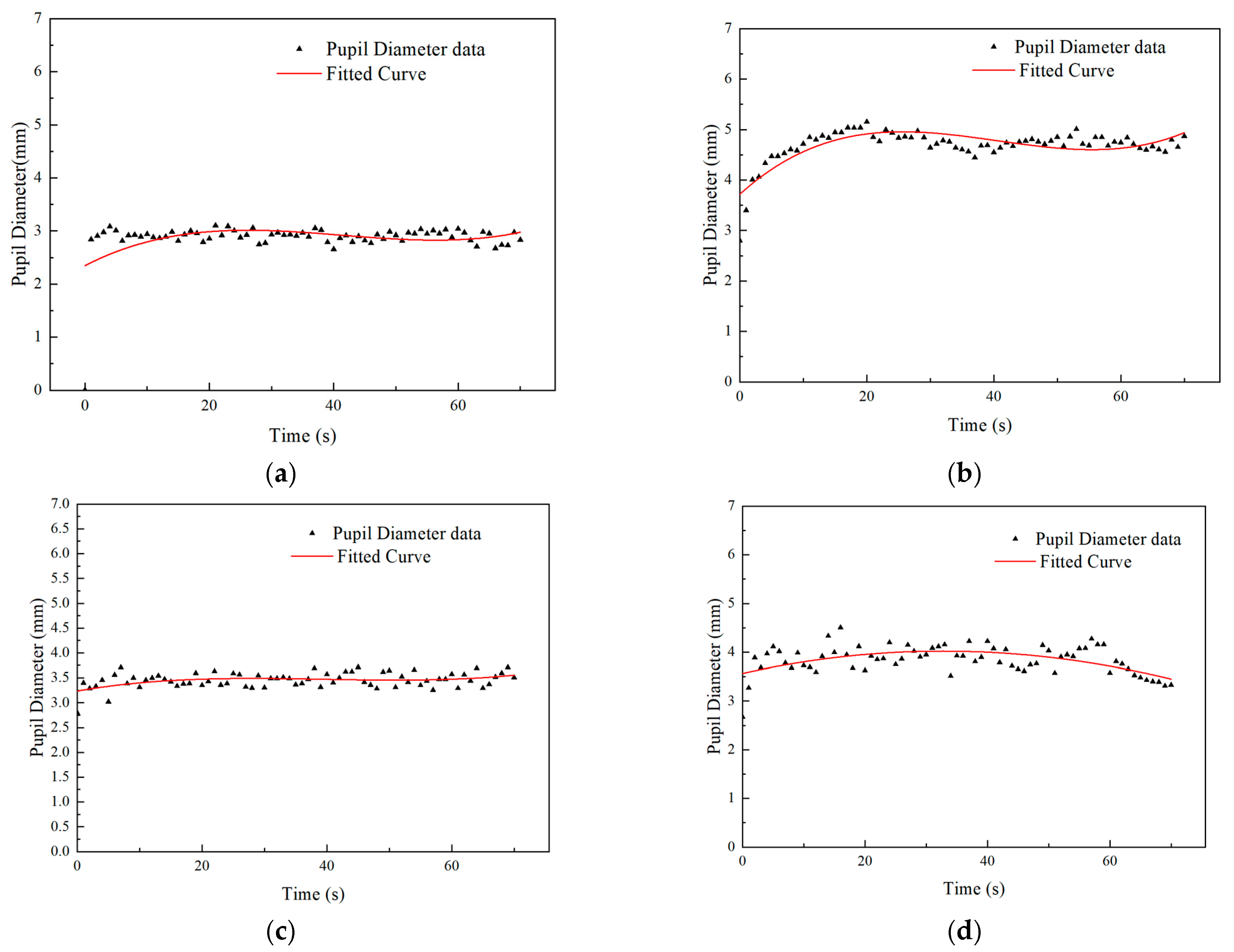
4.2. Modeling of Pupil Diameter over Time at Different Road Sections

The trend of pupil diameter change over time and the fitted curves of drivers in different driving scenarios (straight ahead, turning, climbing, downhill) are shown in Figure 7, which clearly reflect the influence of the complexity of the driving task on the driver’s cognitive load. The fitted model showed better fitting results. The specific fitting parameters are shown in Table 4. The models for the number of fixations under different road sections and their fitting results are listed in Table 4.

For the straight road section, the fitting model is:

$$\mathrm{y}=1.35886\times {10}^{-5}{\mathrm{t}}^3-0.00168{\mathrm{t}}^2+0.06018\mathrm{t}+2.3468$$

(5)

The R² value of this model is 0.813, indicating that the model fitted the data well. The fitted curve for the straight ahead section was smooth, with a smoother change in pupil diameter. This indicated that, in straight driving, the driver’s cognitive load was low, and the driving task was mainly focused on lane keeping, with relatively little attention demand and low environmental complexity. As a result, the pupil diameter changed more slowly and remains in a relatively stable range.

For the turning section, the fitting model is:

$$\mathrm{y}=2.67826\times {10}^{-5}{\mathrm{t}}^3-0.00326{\mathrm{t}}^2+0.11417\mathrm{t}+3.71775$$

(6)

The R² value of this model was 0.772, and the relatively low fitting effect indicated that the pupil diameter fluctuates more in the turning scene and the accuracy of the fitted model was low. At the beginning of the turn, the pupil diameter rose rapidly, which indicated that the driver’s cognitive load increased significantly when facing the tasks of path selection, speed control, and environment judgment. With the completion of the turning task, the cognitive load gradually decreased and the pupil diameter gradually stabilized.

For the climbing section, the fitting model is:

$$\mathrm{y}=5.1995\times {10}^{-6}{\mathrm{t}}^3-6.16309\times {10}^{-4}{\mathrm{t}}^2+0.02224\mathrm{t}+3.235289$$

(7)

The R² value of the model was 0.794, which indicated a better fitting effect for the climbing section. When going uphill, the pupil diameter rose slowly, which reflected the driver’s high demand for power control and speed adjustment at the beginning of the ramp. As the driver gradually adapted to the on-ramp environment, the cognitive load decreased and the pupil diameter stabilizes.

For the downhill section, the fitting model is:

$$\mathrm{y}=1.8722\times {10}^{-7}{\mathrm{t}}^3-4.36681\times {10}^{-4}{\mathrm{t}}^2+0.028\mathrm{t}+3.56532$$

(8)

The R² value of the model was 0.753, and the relatively low fitting effect reflected the high volatility of the data in the downhill section, which lead to the poor accuracy of the model. At the beginning of the downhill section, the pupil diameter rose rapidly, which indicated that the driver faced a cognitive load of controlling speed and responding to potential hazards; however, as the gradient decreases or the environmental complexity decreases, the driver gradually adapted, the cognitive load was reduced, and the pupil diameter decreased.

Overall, the fitted models in

Table 5. Model of the change in pupil diameter for different road sections.

Section of Road	Pupil Diameter Model	${\mathit{R}}^2$
Straight Movement	$y=1.35886{ \times 10}^{-5}{t}^3-0.00168t^2+0.06018t+2.3468$	$0.813$
Turn	$y=2.67826 \times { 10}^{-5}{t}^3-0.00326t^2+0.11417t+3.71775$	$0.772$
Climbing	$y=5.1995\times { 10}^{-6}{t}^3-6.16309\ast {10}^{-4}{t}^2+0.02224t+3.23528$	$0.794$
Downhill	$y=1.8722{ \times 10}^{-7}{t}^3-4.36681\ast {10}^{-4}{t}^2+0.028t+3.56532$	$0.753$

reflected the trends of drivers’ pupil diameters over time in different driving sections, revealing the effect of driving task complexity on cognitive load. In the straight driving section, the lower cognitive load resulted in a smooth change in pupil diameter and a better fit. In contrast, in the complex sections such as turning, climbing, and downhill, the cognitive load of the driver increased, resulting in larger fluctuations in pupil diameter and a poorer fit than that of the straight road section. These results suggested that changes in cognitive load were closely related to roadway complexity, and the cubic polynomial model captured most of the trends better.

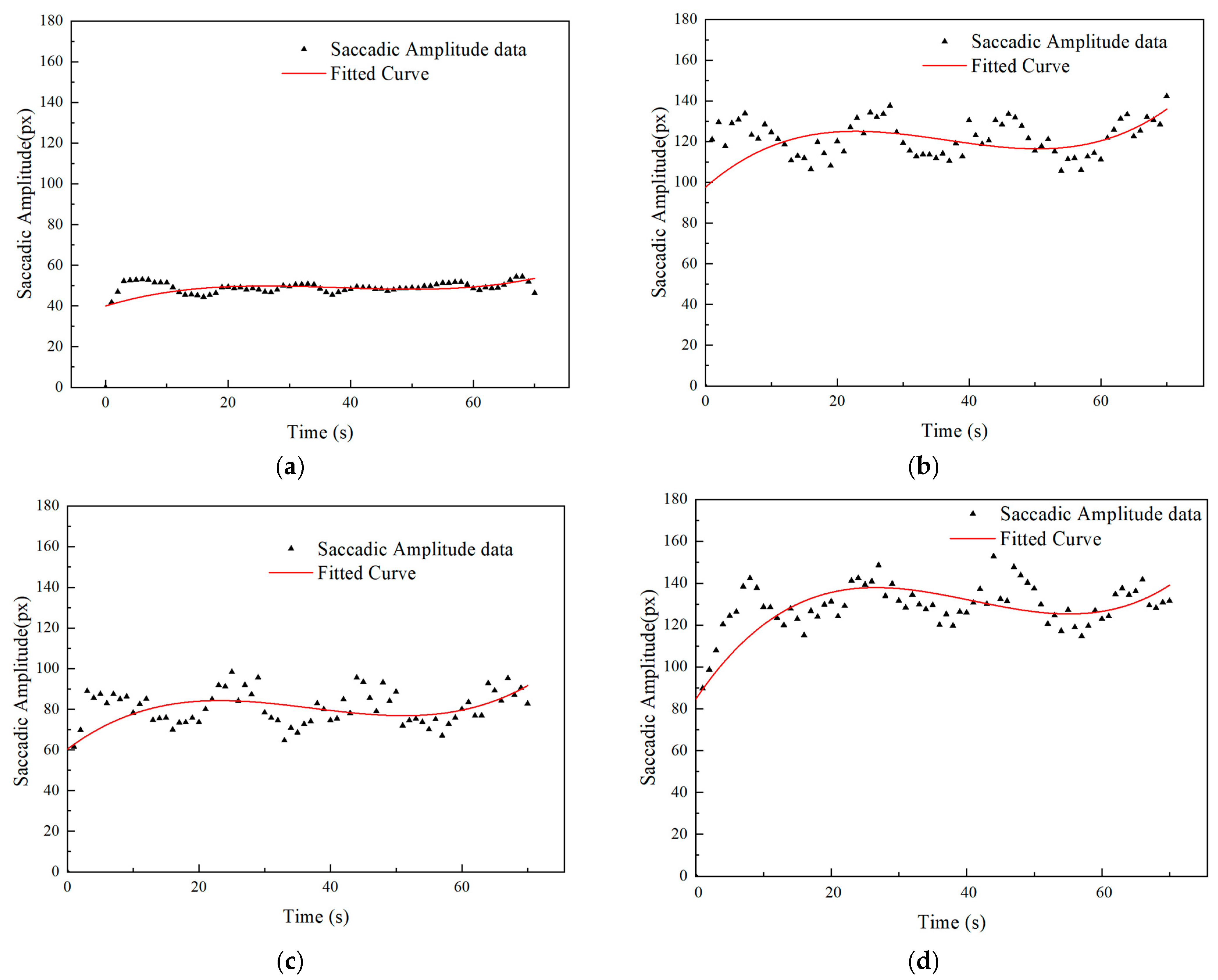
4.3. Modeling of Saccade Amplitude over Time Under Different Road Sections

Figure 8 demonstrated the trend of driver saccade amplitude over time for different roadway conditions. The fitting results are shown in

Table 6. Modeling of saccade amplitude under different road sections.

Section of Road	Saccade Amplitude Model	${\mathit{R}}^2$
Straight Movement	$y=2.35796\times {10}^{-4}{t}^{3 }-0.02682t^2+0.91661t+39.98236$	$0.842$
Turn	$y=8.24778\times {10}^{-4}{t}^3-0.09047t^2+2.83902t+97.6021$	$0.713$
Climbing	$y=6.81582\times {{10}^{-4}t}^3-0.07598t^2+2.42437t+60.45934$	$0.729$
Downhill	$y=0.00108t^3-0.13295t^2+4.77193t+84.71186$	$0.721$

, where the driver saccade amplitude for the three roadway segments, except for the straight roadway segment, exhibited significant volatility.

The fitting model for the straight roadway section is:

$$y=2.35796\times {10}^{-4}{t}^{3 }-0.02682t^2+0.91661t+39.98236$$

(9)

The R² value of this model was 0.842, which indicated a good fitting effect. In the straight road section, the driver’s attention was focused on the centerline of the road ahead, the cognitive load was low, the saccade amplitude was small and stable, and the fitting curve showed a smooth state.

In the turning section, the fitting model is:

$$y=8.24778\times {10}^{-4}{t}^3-0.09047t^2+2.83902t+97.6021$$

(10)

The R² value of the model was 0.713, and the relatively low fitting accuracy indicated that the data were more volatile. During the turning process, drivers needed to frequently shift their eyes to cope with the changing environment and path selection, which resulted in increased saccade amplitude and high volatility.

For the climbing section, the fitted model was:

$$y=6.81582\times {10}^{-4}{t}^3-0.07598t^2+2.42437t+60.45934$$

(11)

The R² value of this model was 0.729, which indicated a relatively poor fitting effect. During the climbing course, the drivers needed to perform power control and speed adjustment, and the saccade amplitude gradually increased with time, but with the adaptation to the ramp, the saccade amplitude gradually stabilized.

For the downhill section, the fitting model is:

$$y=0.00108t^3-0.13295t^2+4.77193t+84.71186$$

(12)

The R² value of the model was 0.721, and the relatively low fitting accuracy indicated that the driver’s saccade amplitude was more volatile during the downhill section, especially in the initial period, when the drivers needed to adjust their vision frequently to cope with the potential speed and hazard control needs, which resulted in a poor model fitting.

Overall, the fitted models in Table 6 showed high prediction accuracy in the straight ahead and climbing segments, while in the turning and downhill segments, the data points fluctuate more, resulting in a poorer fit. This suggested that drivers had increased cognitive loads and greater fluctuations in saccade amplitude in such complex sections of turning and downhill, which affected the model fitting accuracy.

5. Conclusions

In this study, the following main conclusions were drawn from the real-vehicle tests and data analysis of the eye tracking characteristics of 23 drivers on different road sections including straight line, curved road, climbing, and downhill:

(1)

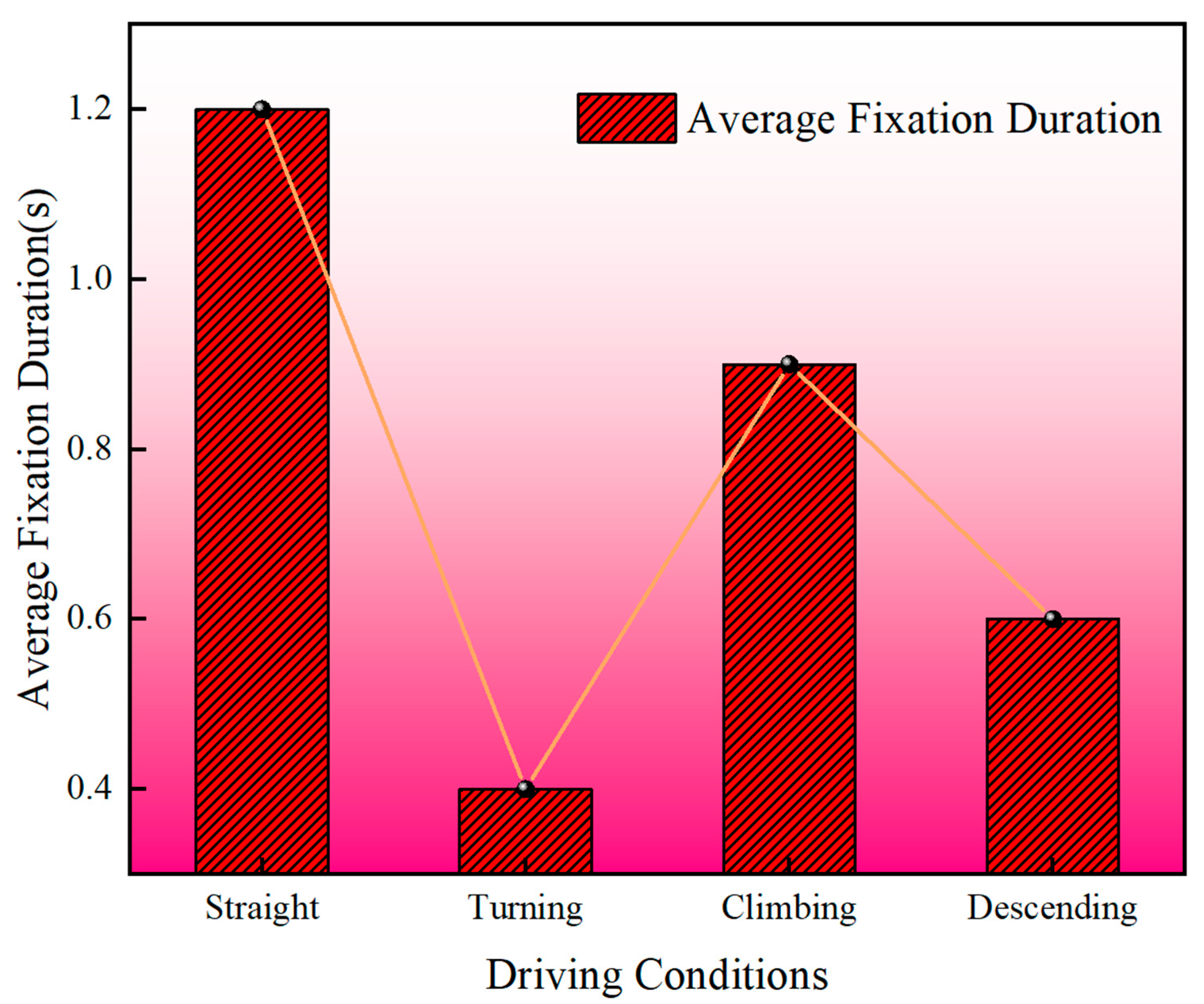
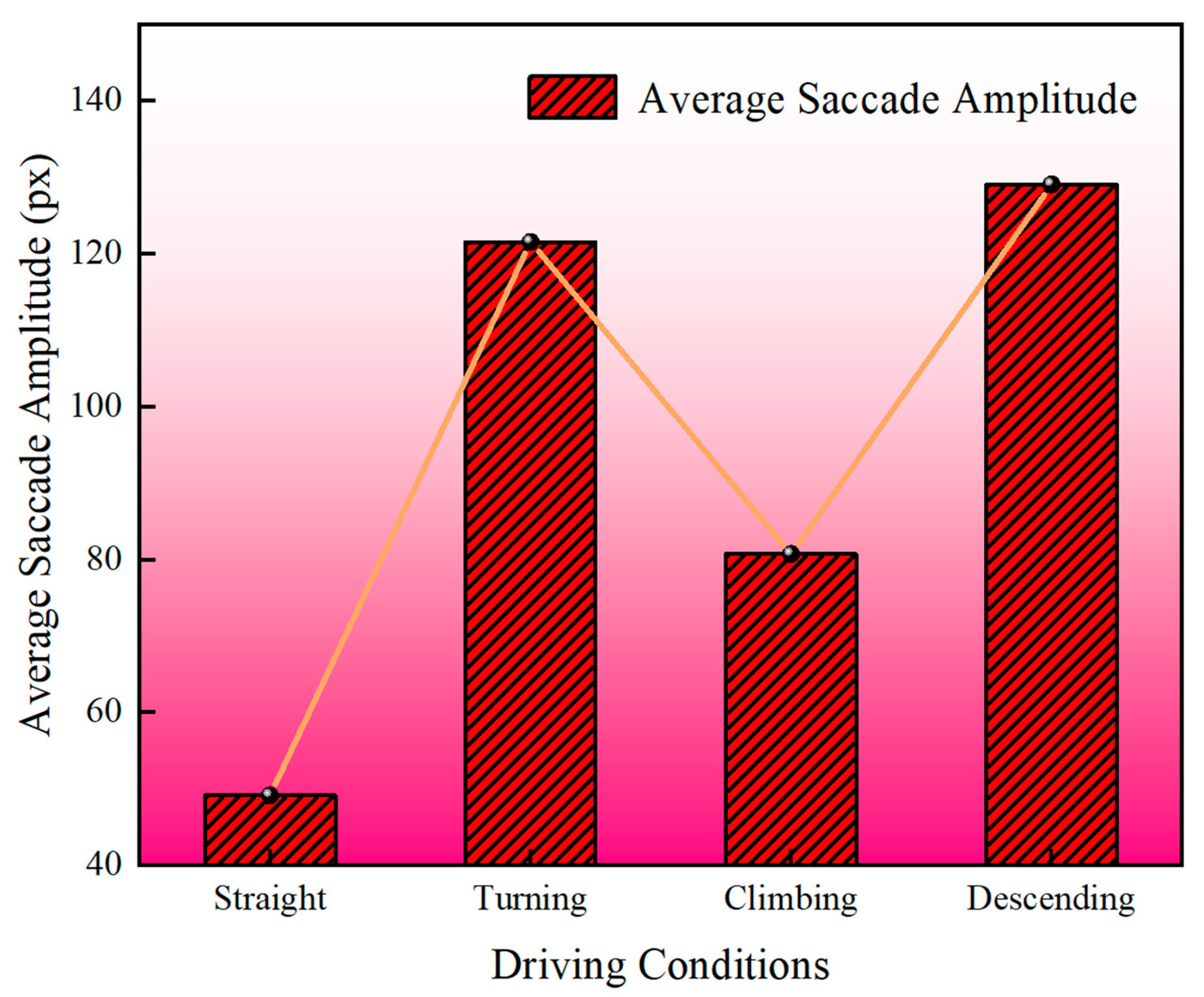
The article revealed the significant effects of different roadway driving tasks on drivers’ eye tracking characteristics and clarified the regular changes of the three indicators of eye tracking characteristics describing the eye movement behaviors of fixation, pupil, and sweep under different roadway conditions. The average fixation duration ranking was found to be straight ahead > climbing > downhill > turning, that of pupil diameter was found to be turning > downhill > climbing > straight ahead, and that of saccade amplitude was found to be downhill > turning > climbing > straight ahead. These results reflected the profound influence of driving task complexity and environmental dynamics on drivers’ visual behavior.

(2)

Drivers’ eye tracking characteristics showed significant variability under different roadway driving tasks. One-way ANOVA results showed statistically significant differences in average fixation duration, pupil diameter, and saccade amplitude under different roadway conditions (p < 0.05). This study provides an important experimental basis for driving behavior modeling, driver state monitoring, and advanced driver assistance system (ADAS) optimization.

(3)

A computer-fitted model of driving time and eye tracking indicators was developed. Based on the experimental data, this paper established a computer-fitted model between driving time and eye tracking indexes, which further revealed the law of visual task allocation of drivers under different road sections. The model was able to quantitatively describe the time-varying characteristics of average fixation duration, pupil diameter, and saccade amplitude of drivers under different road sections and provided theoretical support for the optimization of future traffic safety interventions and advanced driver assistance systems.

In summary, this study, through the systematic analysis of a driver’s visual characteristics, using statistical methods to verify the differences of the driver’s eye tracking characteristics under different road conditions, and through the computer fitting method, quantitatively describes the change rule of the eye tracking characteristics of different road sections, which provides a scientific basis and an important reference for the optimization of road design, traffic safety management, and intelligent transportation systems. However, this study also has some limitations. For example, the sample size of subjects is relatively small, which may not be able to fully reflect the diversity of different driving groups; the selected eye tracking indexes are relatively single and fail to fully integrate other potential key indexes (e.g., the distribution of fixation points and fixation duration), and only a one-way ANOVA was performed; however, considering that factors such as individual driver differences and driving task complexity may interact on eye tracking behavior, subsequent studies will use a two-way ANOVA approach to comprehensively assess the interaction between road conditions and these factors; at the same time, in constructing the eye tracking models under the four road sections, we mainly focused on the characteristics of the changes in the temporal dimension and did not fully take into account the complexity of the spatial environment and the influence of the physiological and individual differences of different drivers. The cubic polynomial model performs well in the fitting effect, but it is a relatively complex model and subsequent studies can explore the use of more simplified models. Future research can expand the sample coverage on this basis and introduce more multi-dimensional and multi-level eye tracking data, such as combining fixation tracking and spatial features, to further explore the comprehensive impact of multi-factor interaction on drivers’ visual behavior. In addition, the interaction mechanism between drivers and automatic driving systems can be explored in conjunction with automatic driving technology, and more precise traffic safety protection strategies can be proposed from the perspective of human–machine synergy, so as to provide more forward-looking research support and practical guidance for intelligent transportation and safe driving.