1. Introduction
From the 1990s to the early 21st century, with the continuous exploitation and utilization of resources, deep concave open-pit mines have become a development trend for open-pit mining worldwide [
1]. Because of the lack of effective landslide early warning methods, it is often impossible to issue timely warnings before landslides occur, resulting in severe casualties and economic losses, which seriously affect mine production and people’s daily lives. Traditional monitoring technologies—such as GNSS [
2], 3D laser scanning [
3], and total stations [
4]—are limited by their single-point data acquisition modes [
5,
6] and delayed data processing mechanisms [
7,
8,
9], making it difficult to fully capture the spatiotemporal evolution characteristics of slope deformation.
In recent years, slope radar has emerged as an important technical means for identifying, determining, and predicting landslide deformation fields because of its advantages of high-precision measurement, large-scale monitoring capability, and all-weather microwave remote sensing technology [
10,
11,
12]. Existing early warning models primarily emphasize the temporal variation in displacement [
13] while neglecting spatial correlations between monitoring points. In practical engineering applications, this often leads to insufficient accuracy in identifying deformation zones and an inability to accurately reflect the spatial distribution of slope deformation. Moreover, current methods lack consideration of the detailed evolution characteristics of displacement, making it easy to misinterpret isolated outliers caused by local disturbances or equipment errors as deformation signals. Such misjudgments not only increase the false alarm rate but may also obscure actual deformation trends, thereby undermining the reliability of early warning results. Therefore, to address this issue, this study employs the Density-Based Spatial Clustering of Applications with Noise (DBSCAN) algorithm to identify and select clusters of monitoring points with significant displacement and a certain degree of spatial distribution as early warning units.
The analysis of displacement curves within early warning units is complicated by the significantly non-stationary nature of slope displacement sequences, which results from the coupling of topographic, structural, and hydrogeological factors. Their evolution involves two key dynamic mechanisms: (1) long-term trend deformation dominated by geological structural stress, representing the long-term evolution of time-dependent damage accumulation in the rock mass, and (2) quasi-periodic responses induced by cyclical environmental disturbances (such as rainfall infiltration), reflecting the recurring effects of seasonal hydrological cycles. This multi-scale coupling feature poses fundamental challenges to traditional single-model prediction approaches: when a single model is used to directly fit the original displacement sequence, high-frequency noise can mask the underlying trend, while low-frequency trends may interfere with the extraction of periodic features, ultimately limiting the generalization capability of the predictive model. To address this issue, some researchers have proposed a “decomposition–prediction–reconstruction” framework, in which landslide displacement is first decomposed into different components, separate models are constructed for each component, and the results are finally reconstructed by summation to improve both prediction accuracy and model adaptability.
In the decomposition of displacement, traditional methods typically use wavelet analysis, empirical mode decomposition (EMD), and ensemble empirical mode decomposition (EEMD). For example, Li et al. [
14] introduced wavelet analysis in their study of surface subsidence pattern recognition in underground metal mining areas. They analyzed the frequency variations in SBAS-InSAR-derived subsidence time series, identifying low-frequency signals to locate zones of stable subsidence and using high-frequency components to capture the frequency and amplitude of sudden deformation events. Zhou et al. [
15] applied wavelet analysis to decompose landslide displacement series into components with distinct frequency characteristics, based on an analysis of the chaotic nature of the displacement time series. Huang et al. [
16] investigated the displacement sequence at monitoring point D3 of the Baijiabao landslide, decomposing the original displacement series into low-, medium-, and high-frequency components using wavelet transform; the lowest frequency term was treated as the trend component, while the sum of the remaining terms represented the periodic component. Xu et al. [
17] adopted empirical mode decomposition (EMD) to divide cumulative displacement into trend and periodic components, successfully extracting rainfall-related intrinsic mode functions (IMFs), which improved the performance of subsequent Long Short-Term Memory (LSTM)-based prediction. Zhang et al. [
18] proposed a soft-sifting-criterion-optimized EMD approach, integrating K-means clustering and an FOA-LSSVM model to effectively predict “step-like” landslide displacements. While the model enhanced both the interpretability and accuracy of prediction, the method required complex parameter optimization. Yuan et al. [
19] focused on the deformation characteristics of step-like landslides and used EMD to separately decompose multi-point monitoring data into trend and periodic components. To address the non-stationarity of displacement data, Liu et al. [
20] employed ensemble empirical mode decomposition (EEMD) and embedded the decomposed features into a Convolutional Neural Network (CNN)–LSTM hybrid model, significantly boosting prediction accuracy. Kang et al. [
21] utilized EEMD to reconstruct displacement series into physically interpretable trend and fluctuation components for spoil slopes with nonlinear and small-sample characteristics, thereby improving prediction robustness. Deng et al. [
22] applied EEMD to decompose the surface displacement time series of the Baishuihe landslide into trend and fluctuation components, further illustrating the effectiveness of the method. Although these methods have achieved certain successes, they also exhibit notable shortcomings: for example, wavelet analysis relies on the empirical selection of basis functions, which limits its ability to capture the non-stationary characteristics of slope displacement and may result in energy leakage. EMD employs an adaptive decomposition approach that overcomes the dependency on predefined basis functions, but it still suffers from severe mode mixing and end effects, which can distort the decomposition results. EEMD introduces white noise and performs ensemble averaging to effectively mitigate mode mixing, yet it incurs high computational costs, and residual noise may still interfere with the accuracy of low-frequency components. Therefore, to address the limitations of the existing methods, after identifying early warning units using the DBSCAN algorithm, this study adopts Variational Mode Decomposition (VMD) [
23] to decompose the landslide displacement within these units into trend and periodic components with clear physical interpretations [
24]. Compared to traditional methods, such as wavelet analysis, EMD, and EEMD, VMD offers superior adaptability and frequency-domain constraints, effectively mitigating mode mixing while ensuring stable and controllable decomposition outcomes—making it well suited for handling non-stationary and nonlinear slope displacement data.
In terms of prediction models, traditional machine learning methods have been widely used. Li et al. [
25] proposed a dynamic interval prediction method for landslide displacement based on the random forest algorithm, which enhanced prediction accuracy and reliability by automatically identifying deformation states and incorporating a state-transition model. Senanayake et al. [
26] developed a regression-based machine learning approach using 3D photogrammetric models of open-pit highwalls to rapidly predict rockfall energy and run-out distances. Zhang et al. [
27] applied ensemble learning techniques (RF and XGBoost) to slope stability prediction, achieving higher accuracy compared to support vector machines and logistic regression. Kardani et al. [
28] employed a hybrid stacking ensemble method optimized by the artificial bee colony (ABC) algorithm, integrating finite element-derived synthetic data with 107 field cases, and achieved a prediction AUC of 90.4%, significantly outperforming single machine learning models (maximum AUC 82.9%) and basic ensemble methods. However, traditional machine learning models remain essentially static, suffering from limited modeling capacity, an inability to capture temporal dependencies, and high computational complexity.
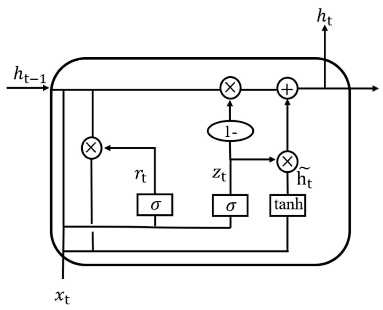
With the rapid advancement of deep learning technologies, LSTM and Gated Recurrent Unit (GRU) models have overcome the gradient vanishing and explosion problems associated with recurrent neural networks (RNNs). These models, which process data sequentially over time, are well suited for time series prediction tasks and have seen widespread application in various fields in recent years [
29]. Xie et al. [
30] employed LSTM to predict the periodic displacement of landslides, finding that LSTM exhibited excellent dynamic properties. Xing et al. [
31] applied LSTM in displacement prediction for the Baishuihe landslide, demonstrating that LSTM outperformed the Extreme Learning Machine (ELM) in terms of prediction accuracy. Yang et al. [
32] applied LSTM to landslide displacement analysis, revealing that compared to static models, LSTM better captured the dynamic characteristics of landslides and effectively utilized historical data. Zhang et al. [
33] developed a landslide displacement prediction model using GRU and applied it to the Diaohuo landslide in the Three Gorges area, showing that GRU offered higher prediction accuracy than the Support Vector Machine (SVM). Zhang et al. [
34] further applied GRU to predict displacement at the Jiuxianping landslide, demonstrating its superior performance in capturing dynamic displacement features and providing a more accurate representation of the Jiuxianping landslide’s deformation, with fewer outliers compared to static models. Inspired by previous studies, this research applies both LSTM and GRU models to displacement prediction and further introduces representative models, such as Temporal Convolutional Network (TCN), RNN, and Autoregressive Integrated Moving Average (ARIMA), for comparative analysis, aiming to systematically evaluate the performance of different modeling approaches in capturing displacement patterns.
This study focuses on the south slope of the main pit in the Bayan Obo open-pit mine. After identifying early warning units using the DBSCAN algorithm, the landslide displacement data of these units are decomposed by VMD into trend and periodic components with clear physical significance. The GRU model is then used to predict the trend component, while the LSTM model is applied to the periodic component. The final displacement prediction is obtained through weighted reconstruction to improve overall accuracy.
Accordingly, the objective of this study is to address the high rates of false and missed alarms by fully considering the spatiotemporal distribution characteristics of slope deformation. A displacement prediction framework is established to improve forecasting accuracy and to assign explicit physical meanings to the decomposed components. This work provides a novel solution to critical challenges in open-pit slope monitoring, particularly the inadequate consideration of spatiotemporal correlations and the difficulty in modeling multi-scale non-stationary sequences in conventional early warning systems.
3. Results
3.1. Cluster Characterization and Result Analysis
Using the optimized clustering parameters obtained from parameter tuning—eps = 3.94 and MinPts = 70—the radar displacement point cloud data were clustered. Based on the clustering results, several clusters of monitoring points were identified according to their spatiotemporal features. Each cluster was labeled in a different color to facilitate a detailed analysis of the clusters with the highest mean cumulative displacement and the largest area.
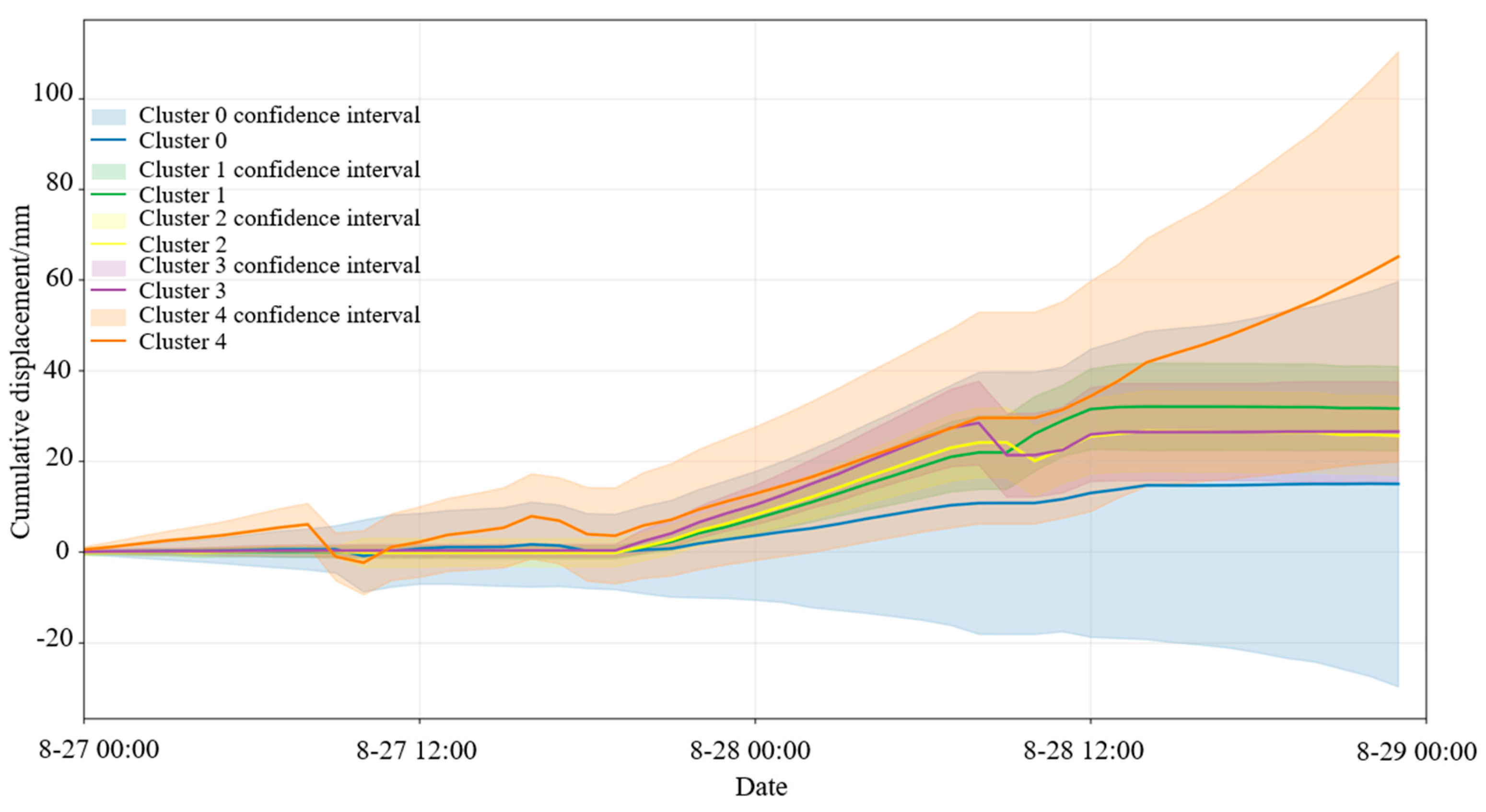
Figure 8 shows the clustering results of radar monitoring data from the slope. As seen in the figure, six clusters were identified from the Bayan Obo Mine southern slope radar monitoring point cloud, with Cluster −1 being classified as noise. Except for Clusters 0 and 4, the remaining clusters have relatively small surface areas and limited impact on overall slope stability.
By observing the clustering cloud map, it can be seen that there are clusters with a larger number of points and greater cumulative displacement between the 1650 m and 1570 m platforms. Among them, Cluster 4 is located between 1570 m and 1626 m. The displacement time series curve of this cluster is shown in
Figure 9.
It is relatively clear from the above figure that the southern slope experienced a slow–rapid–accelerated deformation phase between 27 August and 29 August. All six clusters showed relatively small cumulative displacements in the early stage. Around 18:00 on 27 August, the displacement change of Cluster 0 began to lag behind the other five clusters. From 12:00 on 28 August onward, the cumulative displacement of Cluster 4 began to increase significantly, reaching over 60 mm on 29 August—the maximum displacement before the landslide occurred. According to the resistivity profile and geological cross-section along the survey line, the area where Cluster 4 is located contains a fault fracture zone and an adverse-dip structural plane, with a high degree of weathering. Under the combined influence of these factors, the slope in this area became unstable, which explains why Cluster 4 exhibited the greatest displacement.
These results indicate that the proposed method leverages the spatiotemporal continuity of radar remote sensing data from the slope surface, effectively avoiding false alarms caused by monitoring data from small areas or isolated points. It also allows for more accurate monitoring and early warning of landslide scale and deformation stages.
As shown in the figure, Cluster 4 exhibits the largest mean cumulative displacement, and its displacement curve shows non-stationary characteristics. In the subsequent analysis, VMD will be applied to decompose the displacement curve of Cluster 4. The low- and mid-frequency components after decomposition will be predicted using the GRU and LSTM neural networks in order to reveal the characteristics of their displacement evolution.
3.2. Slope Displacement Decomposition Results
The parameters for VMD decomposition were optimized using PSO. The specific parameter settings are shown in
Table 3, and the PSO optimization results are presented in
Table 4.
Using the optimized parameters, the total displacement was decomposed into trend component displacement (reflecting long-term trends influenced by geological conditions like lithology and structure) and periodic component displacement (driven by external factors such as rainfall).
The decomposition effect of trend component displacement is shown in
Figure 10. As seen in the figure, the trend component displacement curve is smoother than the original displacement curve, with high-frequency components removed. The original displacement curve exhibits several minor declines, while the trend component does not follow these declines, indicating that VMD successfully filtered out short-term disturbances and focused on long-term trends. The close alignment between the trend component and the original curve demonstrates a clear and rapidly increasing trend during this stage.
The decomposition effects of periodic component displacement and rainfall data are shown in
Figure 11. The periodic component displacement curve exhibits intense fluctuations with multiple peaks, representing high-frequency disturbance components. The current rainfall period shows multiple significant surges in rainfall, which align with the abrupt fluctuations in the displacement curve. The proximity of peaks between the two curves indicates that the current rainfall has a notable triggering effect, rapidly increasing the surface moisture content and pore water pressure, thereby inducing displacement disturbances. Rainfall fluctuations from the previous two days exhibit similarities to the displacement curve two days later, reflecting the lagged effect of rainfall.
The southern slope of the Bayan Obo Iron Mine features well-developed joint fractures and fault structures, along with water-sensitive minerals such as mica and montmorillonite. These minerals undergo disintegration and volume expansion upon water contact, confirming the significant impact of rainfall on landslide displacement. To visually quantify the correlation between rainfall and periodic component displacement, Grey Relational Degree analysis was employed. The specific workflow included using periodic component displacement, current rainfall, and prior two-day rainfall as input data; normalizing the data; calculating difference sequences and extremum values; and using these results to compute relational coefficients and GRD. A resolution coefficient ρ=0.5 was introduced to balance sensitivity and stability. The relationship between current rainfall, prior two-day rainfall, and periodic component displacement is illustrated in the figure, with GRD results listed in
Table 5. The GRD values for current rainfall and prior two-day rainfall relative to periodic component displacement are 0.7008 and 0.5770, respectively, both exceeding 0.5, indicating strong correlations.
3.3. Trend Component Displacement Prediction
The training progress is shown in
Figure 12, where RMSE and loss decrease and stabilize with increasing iterations.
Figure 13 displays the prediction results, with the evaluation metrics shown in
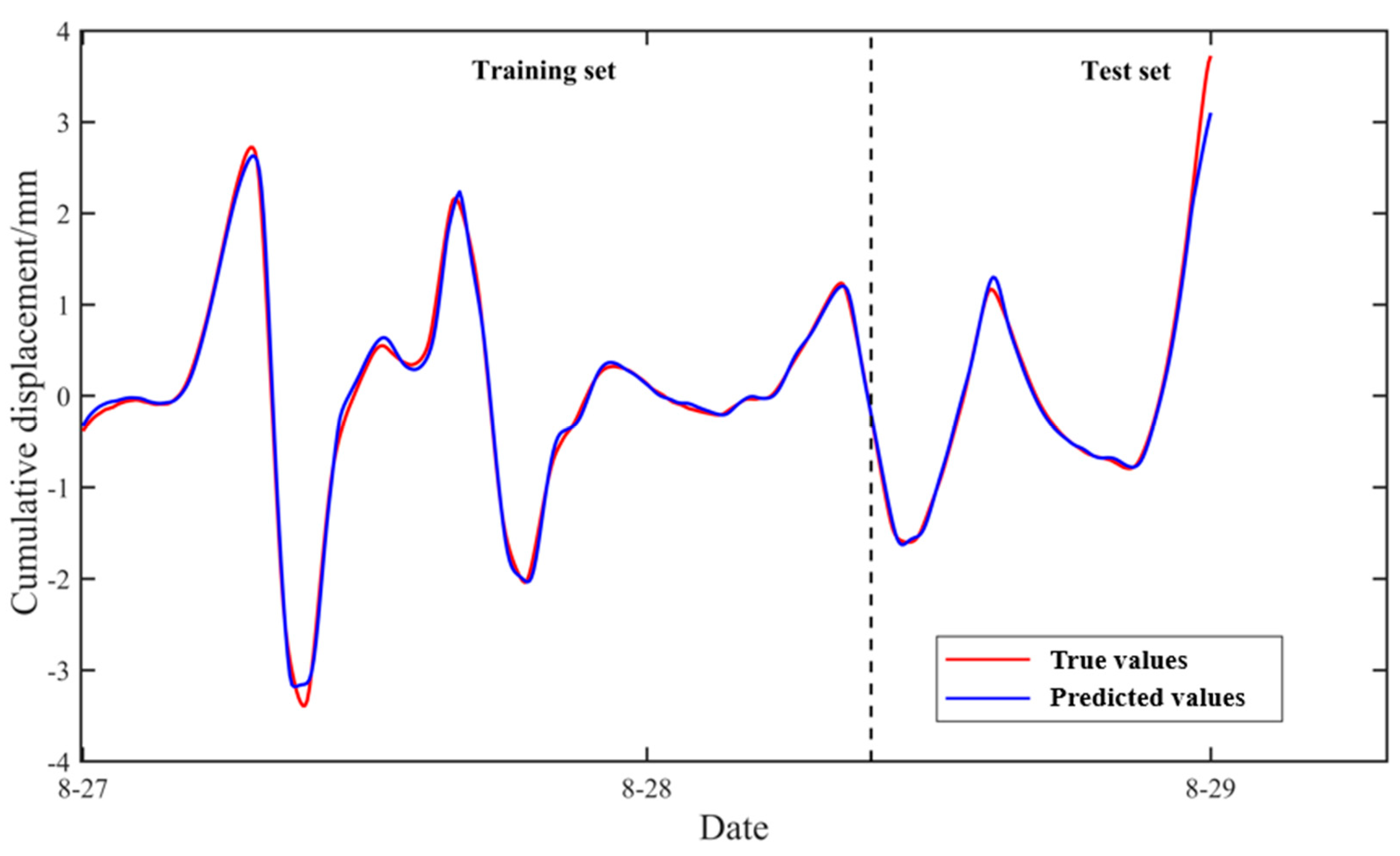
Table 6. RMSE = 0.94794, MAE = 0.46536, and R
2 = 0.99755 validate the effectiveness of the GRU network in trend component prediction. During the training phase, the predicted and true values align closely, with nearly overlapping curves, indicating strong fitting capability on existing data. In the testing phase, despite using unseen data, the prediction curves closely match the true values with accurate overall trends, demonstrating robust generalization. Even in phases with rapid changes, GRU maintains stable trend tracking with minimal errors.
To further validate the GRU model’s performance, comparisons were made with the ARIMA, LSTM, and TCN models under the same dataset, as shown in
Figure 14. GRU consistently adheres to the true value curve throughout the prediction period, particularly excelling in rapid growth phases with superior trend capture capability. Quantitative metrics (
Table 7) show that GRU’s RMSE (0.94794) is significantly lower than the RMSE values of the other models, indicating minimal prediction error. Its R
2 (0.99755) reflects near-perfect data variation explanation, while its MAE (0.46536) confirms the smallest average deviation from observed values. All models perform similarly in the early stages, but during rapid late-stage growth, ARIMA exhibits clear underfitting due to limited linear modeling for complex nonlinear sequences. The LSTM predictions are systematically low with delayed responses at trend inflection points, suggesting potential overfitting or insufficient learning. TCN fails to capture rapid displacement increases, revealing inadequate mid-to-long-term trend modeling.
3.4. Periodic Component Displacement Prediction
Since the data were normalized before training, the prediction results needed to be rescaled back to their original scale for comparison with the true values.
Figure 15 and
Figure 16 display the predicted results, and the corresponding evaluation metrics—RMSE, R
2, and MAE—are presented in
Table 8. For the LSTM model, the RMSE and MAE on the training set are 0.0816 and 0.0585, respectively, with an R
2 value of 0.9948, indicating an excellent fit to the training data and demonstrating the model’s strong ability to capture temporal patterns.
On the test set, while the RMSE and MAE increase slightly to 0.1278 and 0.0635, and R2 drops to 0.9873, the performance remains at a high level, showing that the model maintains strong generalization and prediction capability when dealing with unseen data. For the entire dataset, the overall RMSE and MAE are 0.0978 and 0.0600, respectively, and R2 reaches as high as 0.9925, further validating the effectiveness of the LSTM network in periodic component prediction.
To intuitively evaluate the prediction performance of LSTM, three other models were used for comparison: RNN, GRU, and CNN. The prediction results are shown in
Figure 17, and their evaluation metrics are listed in
Table 9.
From both the figure and the table, it is clear that LSTM achieves the best prediction performance. Its predicted values are the closest to the actual observations, indicating that LSTM’s gating mechanism (forget gate, input gate, output gate) is highly effective in capturing long-term periodic patterns and mitigating gradient vanishing problems. LSTM has the lowest RMSE and highest R2, suggesting that it nearly perfectly fits the data.
GRU, with its simplified gating structure (update and reset gates), performs well on periodic sequences but is slightly less capable than LSTM when modeling complex periodic dynamics. Compared to RNN and CNN, GRU achieves a lower RMSE and MAE, supporting the effectiveness of gating mechanisms.
The standard RNN model struggles with long-term dependencies due to the gradient vanishing issue, leading to significantly higher errors than LSTM and GRU. Meanwhile, CNN, being more suited for spatial data, is not ideal for purely temporal periodic sequences. Its reliance on local convolution kernels limits its ability to directly capture global periodic patterns.
3.5. Total Displacement Prediction
After separately predicting the trend and periodic components of the displacement, the final landslide displacement prediction for Cluster 4 was obtained by reconstructing and superimposing the results. The total displacement prediction is illustrated in
Figure 18. Quantitative evaluation using RMSE, MAE, and R
2 yields RMSE = 0.9948 mm, MAE = 0.4960 mm, and R
2 = 0.9973, indicating a high level of overall prediction accuracy.
4. Discussion
In multi-scale landslide displacement modeling, the quality of signal decomposition directly influences the stability and interpretability of prediction results. Compared to traditional methods, such as EMD, EEMD, and wavelet analysis [
14,
15,
16,
17,
18,
19,
20,
21,
22], the VMD approach adopted in this study demonstrates significant advantages. It distinctly separates displacement sequences into a long-term trend component controlled by geological structures and a high-frequency periodic component influenced by rainfall disturbances, thereby providing physically meaningful intrinsic modes for subsequent modeling. Unlike EEMD, VMD eliminates the need for multi-round perturbation superposition and reconstruction during decomposition, resulting in higher computational efficiency. This makes it more suitable for rapid early warning modeling in practical engineering scenarios. Furthermore, the framework’s robust predictive performance confirms the superiority of VMD, demonstrating reliable capabilities in real-world slope monitoring applications.
For predictive modeling, this study employs a hybrid “trend component-GRU, periodic component-LSTM” strategy, which shows notable advantages over existing approaches that uniformly apply a single network model to all components. For instance, Xie et al. [
30], Xing et al. [
31], and Yang et al. [
32] utilized LSTM models for full displacement sequence modeling, while Zhang et al. [
33,
34] applied GRU models to holistically predict landslide displacement. While these methods exhibit certain predictive capabilities in handling complex temporal data, they fail to distinguish the dynamic differences between trend and periodic components, often leading to feature ambiguity or structural underfitting during modeling. Through our component-specific matching strategy, the GRU model achieves an R
2 value of 0.99755 in trend component prediction, significantly outperforming comparative models including ARIMA, TCN, and even LSTM (
Table 7). This highlights GRU’s advantages in capturing slow-varying trends with fewer parameters and faster convergence. Simultaneously, the LSTM model attains the lowest RMSE (0.0978 mm) in periodic component prediction, surpassing the traditional RNN, CNN, and GRU models (
Table 9), demonstrating its strength in modeling complex periodic disturbances and high-frequency responses. The final PSO-VMD-GRU/LSTM framework achieves an overall displacement prediction R
2 of 0.9973, further validating the effectiveness of component-specific modeling in enhancing prediction accuracy and model generalization capabilities.
Although the proposed framework is constructed based on data from the Bayan Obo open-pit iron mine, its core methodology exhibits strong transferability. Notably, the DBSCAN algorithm identifies early warning units through spatiotemporal density distributions of monitoring points, independent of specific geological types. This makes the method applicable to other open-pit mine slopes with dense displacement monitoring data. However, broader implementation requires careful consideration of the following prerequisites: First, the method depends on high-temporal-resolution monitoring data as foundational support. This study utilizes hourly interval, ground-based radar data comprising 114,283 monitoring points, each containing 48 h of continuous displacement records, which provide the necessary data integrity for VMD decomposition and periodic feature extraction. It should be noted that the decomposition results and subsequent prediction model performance would be significantly degraded under conditions of sparse sampling intervals, data discontinuity, or abnormal missing values. Second, the prediction of periodic components is highly dependent on rainfall as an external driver. However, the rainfall–displacement coupling relationship is not universally applicable. In regions with minimal rainfall fluctuations, arid climates, or complex hydrogeological conditions, this coupling may exhibit weak correlations or significant time lags, necessitating the introduction of alternative drivers, such as groundwater levels or hydraulic pressures, or structural model adaptations to accommodate regional characteristics. Third, lithological characteristics fundamentally govern slope response mechanisms to external disturbances. The rock mass in the Bayan Obo mining area primarily contains water-sensitive minerals (e.g., mica, montmorillonite) with developed joint fractures. In contrast, regions with homogeneous lithology, compact structures, or dry stable conditions often show atypical rainfall-induced displacement responses, leading to difficulties in periodic component extraction and reduced prediction model stability. Finally, the framework exhibits sensitivity to multiple critical parameters: DBSCAN’s ε and MinPts settings, VMD’s mode number selection, and hyperparameter configurations in LSTM/GRU networks. Optimal parameter combinations may vary substantially across regions. Therefore, during implementation, cross-validation or sensitivity analysis should be conducted based on regional geological and climatic features.
To assess the computational feasibility of the proposed method for near-real-time warning systems, this study evaluates the computational demands of the PSO-VMD algorithm and the training efficiency of deep neural networks. On a standard computer equipped with an Intel Core i5-13400F CPU and 16GB RAM, the PSO-VMD algorithm completes one parameter optimization cycle (with particle swarm size set to 10 and maximum iterations to 100) in approximately 30 s on average, demonstrating low resource consumption without reliance on GPUs or high-performance servers. Under identical hardware conditions, the training processes of both LSTM and GRU models are completed within 1 min. Comprehensive tests confirm that the method achieves high prediction accuracy with low computational demands and rapid response times, meeting the essential computational performance criteria of near-real-time landslide early warning systems.
5. Conclusions
This study addressed the limitations of traditional landslide early warning methods in open-pit mines, specifically their insufficient consideration of spatiotemporal correlation and the challenges in modeling displacement sequences with multi-scale coupling. To tackle these issues, a novel landslide prediction framework was proposed, integrating DBSCAN clustering with PSO-VMD for multi-scale decomposition.
Using the southern slope of the Bayan Obo main open-pit mine as the research area, and leveraging the spatiotemporal continuity of radar monitoring data, high-risk deformation regions were identified through DBSCAN clustering. Combined with PSO-VMD decomposition and hybrid prediction models, the framework successfully revealed the multi-scale dynamic mechanisms underlying slope displacement evolution. The main conclusions are as follows:
1. By applying a parameter-optimized DBSCAN algorithm to radar point cloud data, Cluster 4—characterized by high average cumulative displacement and wide spatial distribution (located in the 1598–1626 m platform zone)—was successfully identified. This method effectively suppressed outlier interference, and the resulting early warning outputs closely matched the actual spatial–temporal patterns of the landslide.
2. The displacement of Cluster 4 was decomposed into trend and periodic components using VMD optimized by PSO. The trend component captured long-term displacement evolution, with the GRU model achieving a high prediction accuracy (R2 = 0.99755). The periodic component reflected the nonlinear response to hydrological disturbances, and the LSTM model achieved a superior performance with RMSE = 0.0978 mm, significantly outperforming the RNN, GRU, and CNN models. The reconstructed total displacement prediction reached an R2 of 0.9973, further confirming the effectiveness of the multi-scale decomposition framework.
Despite the above results, several limitations remain in the present study. While the Discussion Section highlighted potential challenges in applying the proposed framework to different geological contexts, the current stage of this research still presents certain limitations—particularly in terms of model validation. The proposed framework currently relies on radar displacement curves as the primary validation source. Although manual field inspections prior to the landslide revealed surface cracking and ground bulging in the predicted high-risk area (Cluster 4), no quantitative ground-based monitoring data were available for independent verification. In future work, we plan to incorporate GNSS-based displacement measurements, geological mapping, groundwater sensors, and crack meters to further enhance the model’s stability and generalizability under complex geological and hydrological conditions. Moreover, future developments may explore embedding the framework into real-time monitoring systems to support timely decision-making in mine slope management.
The proposed “Spatiotemporal Clustering–Multi-Scale Decomposition–Hybrid Prediction” framework enables the identification of landslide-prone regions on larger spatial scales and enhances both the accuracy and robustness of displacement prediction. This method offers a promising new technical solution for improving precursor identification of slope instability and ensuring the safety of slope monitoring in open-pit mining operations.


