Abstract
Lamb waves offer a series of desirable features for Structural Health Monitoring (SHM) applications, such as the ability to detect small defects, allowing to detect damage at early stages of its evolution. On the downside, their propagation through media with multiple geometrical features results in complicated patterns, which complicate the task of damage detection, thus hindering the realization of their full potential. This is exacerbated by the fact that numerical models for Lamb waves, which could aid in both the prediction and interpretation of such patterns, are computationally expensive. The present paper provides a flexible surrogate to rapidly evaluate the sensor response in scenarios where Lamb waves propagate in plates that include multiple features or defects. To this end, an offline–online ray tracing approach is combined with Frequency Response Functions (FRFs) and transmissibility functions. Each ray is thereby represented either by a parametrized FRFs, if the origin of the ray lies in the actuator, or by a parametrized transmissibility function, if the origin of the ray lies in a feature. By exploiting the mechanical properties of propagating waves, it is possible to minimize the number of training simulations needed for the surrogate, thus avoiding the repeated evaluation of large models. The efficiency of the surrogate is demonstrated numerically, through an example, including different types of features, in particular through holes and notches, which result in both reflection and conversion of incident waves. For most sensor locations, the surrogate achieves an error between 1% and 4%, while providing a computational speedup of three to four orders of magnitude.
1. Introduction
Within the context of Non-Destructive Evaluation (NDE) and Structural Health Monitoring (SHM) applications of thin plate and shell structures, Lamb waves [1] offer several favorable properties. Firstly, their short wavelength enables interaction with small defects and, therefore, facilitates defect detection in early damage stages [2]. Further, compared to bulk waves, they exhibit reduced geometrical damping allowing to cover large areas with only few sensors. Additionally, the availability of commonly used low-cost PZT sensors renders Lamb wave-based SHM schemes accessible for a wide range of applications [3]. Their flexibility allows for monitoring of various defects, such as fatigue cracks [4,5], notches [6,7], delaminations [8,9], or corrosion [10].
Due to their multi-modality and their dispersive nature, Lamb waves form complex patterns. To simplify these patterns, many Lamb wave-based SHM schemes rely on baseline subtraction to obtain only the response influenced by scattering from defects [11]. In order to keep the scattering response simpler [12], the excitation of single modes is often attempted, which can be achieved either through specially designed actuator setups [13] or through specific frequency tuning [14]. However, the localization of defects still calls for advanced analysis methods, which can be largely classified into data-driven and model-based classes.
Popular data-driven methods include Delay-And-Sum (DAS) [15,16,17] approaches and the Sparse Reconstruction (SR) [18,19], while further data-driven methods rely on the Time-Reversal Method (TRM) [20] and the Time of Flight (ToF) [21,22]. More recently, deep learning (DL) approaches have gained ground with respect to more essential data-driven schemes. A comparison of deep learning models developed for the specific task of GW-based defect detection, including Dense Neural Networks (DNNs), Convolutional Neural Networks (CNNs), Recurrent Neural Networks (RNNs), and Long Short-Term Memory (LSTM) networks is given by Rautela and Gopalakrishnan [23]. In a relevant application which considers a single delamination, Azadi et al. [24] used a total of ten Carbon Fiber Reinforced Polymer (CFRP) laminates—nine damaged and one healthy—to train their 1D-CNN. A laser sequentially creates a localized thermal expansion, allowing for broadband excitation in a grid of points. This excitation, in combination with piezoelectric sensors, positioned in three locations, allows for recording of an experimental dataset with more than 2 million measurements. Using this dataset and hyperparameter optimization, the 1D-CNN proves to offer accurate delamination classification from raw signal data. The aspect of training is particularly important in establishing robust DL-based schemes. In this vein, Rautela et al. [25] introduced a two-step detection and localization approach. They specifically trained their 1D-CNNs on data collected from CFRP plates with attached aluminum disks, which are employed to simulate damage. From this dataset, physical features, such as the time of flight, are extracted. In further work, in an effort to reduce the training data, Postorino et al. [26] applied transfer learning with optimal transport on data generated with a numerical model, which was validated with experiments.
In the present work, data-driven methods exploiting the principle of Frequency Response Functions (FRFs) or transfer functions are of special interest, as the FRF forms a central concept in the development of the proposed surrogate. Sun et al. [27] use the concept of electrical transfer functions to verify the rationality of their measurements. Electrical transfer functions are further used by Wang and Shen [28], in the context of the Time-Reversal Method. The transfer function between the excitation and the measured signal is modified in order to compensate for the influence of the transducer. A drawback of their method lies in the necessity for mode separation, which is often not feasible, especially if the distance between the actuator and sensor is small. The surrogate proposed in the present paper shows the ability to track individual modes and, therefore, it allows for detection of specific modes, which reflections at different parts of the model stem from. In the Decomposition of the Time-Reversal Operator and MUltiple SIgnal Classification (DORT-MUSIC) technique, the transfer function is evaluated for a set of sensor–transducer pairs and, based on individual transfer functions, a transfer matrix is constructed. This matrix is decomposed by means of a Singular Value Decomposition (SVD), which allows for extraction of reflectivity characteristic features from signals originating from different sources, e.g., scatterers. To obtain the transfer matrix, He and Yuan [29] used a sensor setup, where the actuators are perpendicular to the sensors, while Fan et al. [30] relied on a single piezoelectric array. To improve the localization of debonding in CFRP-reinforced steel structures, An et al. [31] derived a Waveform Feature Index (WFI) based on changes in the Transfer function. A method to experimentally derive FRF was given by Yang et al. [32], who used the step function as an excitation. They show that this approach is efficient for FRFs up to 900 . A further application of the FRF is in combination with the wave focusing approach. In this approach, the excitation is modified in order to account for the dispersive nature of Lamb waves [33]. Based on the use of the FRF, Yang et al. [34] reduced the number of required physical recordings needed for wave focusing. Furthermore, the utilization of the FRF allows for seamless prediction of the response for varying excitations. This flexibility of the FRF in dealing with various excitations is a key property, which is exploited in the creation of the surrogate proposed in the present paper.
Despite their attractive trait in using minimal prior knowledge, data-driven methods often remain limited to the setups they were trained on. To increase the flexibility of SHM schemes, mechanical knowledge in the form of the governing equations of the wave propagation problem can be introduced [35]. Such model-based approaches come with the bottleneck of a high computational time, particularly for Lamb wave problems, as the high frequencies and short wavelengths involved require fine discretizations in space and time for mesh-based solvers [3,36]. As a consequence of the high associated computational cost, inverse algorithms need to be efficient with respect to the number of required evaluations of the model. Such an approach was introduced by Bürchner et al. [37], who performed Full Waveform Inversion (FWI) for the 1D wave equation. They introduced a scaling factor for the density of the structure, with the scaling factor tending to 0 for void regions and 1 for solid regions. This allows for calculating gradients efficiently during the optimization process. In turn, exploiting these gradients in a gradient-based optimization scheme, leads to a fast convergence of the inverse problem. This approach was extended to solve elastodynamic problems in geophysics applications [38], where scaling is applied on the shear modulus, rather than the density. The robustness of the approach is further demonstrated for a numerical example with artificial noise. Based on the use of density scaling, Bürchner et al. [39] introduced a model-based approach, where the inverse problem is solved in two steps. In the first step, a coarser resolution is used to identify the area of the defects (in the form of voids) and, in a second step, in the area around the defect, the material properties are modeled in a refined manner, to obtain a sharp resolution for the representation of the void. Similarly, the Finite Cell Method (FCM) allows for modeling features in the plate without the use of extensive mesh refinement. This concept was combined with Particle Swarm Optimization (PSO) by Zakian et al. [40] for damage detection and localization. An approach where Reduced Order Models (ROMs) are exploited in the inverse setting was given by Rautela and Gopalakrishnan [41], who used a ROM for the Spectral Finite Element Method (SFEM) in the frequency domain in combination with CNNs for damage detection and RNNs for damage localization. This approach allows for damage detection, localization, and severity estimation.
Despite the efficiency of the demonstrated model-based approaches, the computational toll remains high as long as a high-fidelity model needs to be solved, which prohibits their application in real-time or near-real-time monitoring. ROMs, in contrast, allow for expedited evaluations of the forward model. One class of ROMs is projection-based Model Order Reduction (MOR), where the matrices of the Full Order Model (FOM) are projected into a lower-dimensional space [42]. In this space, the governing equations are solved efficiently, while the solution of the system is subsequently transformed into the original space to recover the full solution. For wave propagation problems, however, the Kolmogorov n-width, which is a measure of the accuracy with which low-dimensional spaces can represent the solution of a high-dimensional problem, decays slowly. Thus, the size of the reduced bases needed to achieve the acceptable levels of accuracy might not lead to substantial computational gains [43]. An efficient use of projection-based ROMs for wave propagation can be realized through local projection bases [44]. Thereby, the initially collected snapshots, based on which projection bases are constructed, are clustered, with a separate basis being constructed for each cluster. This leads to bases of smaller size; however, it also requires the selection of an optimal basis at each time step of the online solution. While projection-based ROMs aim to reduce the number of Degrees of Freedom (DOFs), an alternative approach, proposed by Bigoni [45] aims at reducing the number of linear system solutions required, which are also the most computationally demanding part of such a simulation. To this end, the ROM is evaluated in the frequency domain for the principal frequencies, which are significantly less than the number of time steps that would be required to solve the problem in the time domain. Such a frequency domain-based ROM was used by Bigoni et al. [46] for damage localization. Building on a similar concept, the surrogate demonstrated in the present paper is evaluated in the frequency domain, only for a discrete subset of frequencies of interest. This concept was further applied to develop an ROM based on FRFs for detection of single defects in the authoring team’s previous work [47]. Through geometrical transformations, defects of equivalent FRF values were found, and then, the FRFs are interpolated exploiting the Matching Pursuit algorithm. An alternate approach lies in the idea of decoupling the time and space domains of the underlying differential equations. This approach, named Proper Generalized Decomposition (PGD), is known to avoid the curse of dimensionality [48]. Using this scheme, a global–local model for beams is presented by Yan et al. [49], who model the main parts of the beams using the wave finite element method, while the section around the defect is modeled via conventional finite element method (FEM). Another surrogate, which relies on the combination of Bayesian optimization with a machine learning approach, enables uncertainty quantification with respect to the material parameters in composite plates [50]. Furthermore, in the framework of SHM, Postorino et al. [51] created a metamodel with radial basis functions. As this metamodel can rapidly evaluate the response for different defect locations, it can be combined with PSO to localize damage in a single-defect scenario.
Surrogate models based on ray tracing track individual wave packets through the plate, allowing for gathering further information about the wave packets at the sensor location. The sensor response is then found by summing the single wave packets together. Furthermore, the computational time of such surrogates is independent of the size of the plate. Ray tracing can be performed using the pencil method, where the wave is tracked with an axial ray and a paraxial ray is introduced to track its amplitude [52]. The method is able to model reflections and mode conversion precisely, even at curved edges and allows for modeling wave sources of finite size. This method was extended to model laminate plates [53]. Mardanshani et al. [54] combined the pencil method with the wave finite element method to model wave propagation in plates with joints. In this concept, the wave finite element method models the transition at the joints, while the pencil method tracks the energy of the wave. Based on an analytical scattering model, Xu et al. [55] provide a ROM that uses a dictionary approach for the scattering, which is combined with the modeling of edge reflections through mirroring. Localizing a single defect with this model outperforms the DAS method regarding the necessary receivers to accurately localize the defect. Similarly to this approach, we explore a surrogate with ray tracing, relying on a numerical model to create a dictionary for the scattering behavior. Allouko et al. [56] modeled the scatterer with finite elements and the area of the pristine plate through semi-analytical solutions for half-spaces. The decoupling of the space around a defect (near field) and the far field is also the base of the model introduced by Lozano et al. [57]. They modeled both fields with different versions of the Scaled Boundary Finite Element Method (SBFEM) and coupled the models with the mortar method. Another analytical scattering model was introduced by Briand et al. [58], who explored a damage index based on the amplitude of the scattering model for an estimation of the damage size. A fast analytical predictor is also given by Poddar and Giurgiutiu [59], who split the area around notches and cracks in several different domains and adjust the boundaries of the domains according to the neighboring domains. This model is called Complex Modes Expansion with vector Projection (CMEP).
Generally, as seen in the aforementioned ray tracing models, the scattering behavior of defects and flaws needs to be investigated carefully, as it significantly influences the sensor response. Such investigations have been performed numerically [6,60,61,62,63,64], analytically [61,64] and experimentally [62,63,64] for different types of defects. The results of these analyses indicate that the reflection is dependent on the mode and frequency of the incident wave [63]. Sedaghati et al. [61] derived an analytical formulation for the scattering of the wave mode by coupling the Poisson plate theory with the Mindlin plate theory. They analyzed symmetric and asymmetric double-sided blind holes and concluded that the thickness and the type of the hole are relevant to the scattering behavior. This, in turn, reveals that conclusions on the size and type of defects can be drawn on the basis of characteristics of the scattering signals. In their paper, they provide a summary of further analytical solutions of the wave scattering phenomena for different types of defects. The investigation of the -mode shows that the Scattering Directivity Pattern (SDP) is asymmetric for angled cracks [6] and that for some angles of incident waves, there are no reflections [62]. The latter seems to also be apparent for the circular defects investigated in the present paper. Fromme and Rouge [62] concluded that angles with no reflections need to be considered when designing and mounting an SHM system. Further, Soleimanpour and Soleimani [60] investigated the clapping phenomenon for cracks in an aluminum plate for the -mode. The clapping leads to a nonlinearity in the scattering behavior, which creates higher harmonics. The paper focuses on the first two harmonics. It shows that the observed nonlinear effects are well suited for damage detection. If a setup where linear waves are investigated is used, they recommend using a pitch-catch configuration, where the actuator and the sensor are in different sides of the defect. In the present contribution, we will focus on linear waves that are indeed examined in such a pitch-catch setup. In their study on waves with cylindrical holes, Diligent et al. [64] investigated relations between the size of the defect and the scattering coefficient, as well as between the distance from the defect and the scattering coefficient. The latter relation is described through a simple formula, reflecting geometrical damping, which is used herein to find the scattering waves for sensors at any distance to a scatterer.
In the current paper, a novel approach is proposed, which combines several of the aforementioned aspects, to achieve flexible surrogate models that are able to predict the sensor response in plates with several flaws. An online–offline approach is adopted, where the scattering behavior for different flaws is firstly learned in the form of transmissibility functions and next stored in a dictionary during an offline phase. The created dictionary of transmissibility functions is integrated in a ray tracing approach, allowing for consequently evaluating the sensor response.
The remainder of the paper is structured as follows. In Section 2, the theory underlying the surrogate is presented, followed by the description of the proposed approach in Section 3, pertaining to both the online and offline phase of the model, including algorithmic implementation details. In Section 4, the method is demonstrated on a numerical example and results for two different kinds of defects are investigated. The paper is concluded by a discussion on the advantages and limitations of the model and an outlook on further research.
2. Theory
2.1. Lamb Waves
Lamb waves are multi-modal waves propagating in thin plates, which means that, generally, more than one mode is propagating (Figure 1), with an infinite number of these modes existing in theory. Generally, these modes are classified, based on the resulting stress distribution along the cross section, into symmetric and anti-symmetric modes [65]. However, most modes comprise a cut-off frequency below which they do not propagate. The cut-off frequencies depend on the material and thickness of the plate. Two Lamb wave modes, the fundamental symmetric, , and the fundamental anti-symmetric, , modes exist, which propagate across all frequencies [66]. For most Structural Health Monitoring (SHM)-applications, the excitation is chosen so that they operate at the frequency range where only these two fundamental modes propagate [8,21,67]. In the presence of perturbations within the plate, such as defects [68] or in the presence of boundaries [69], mode conversion can occur. Furthermore, Lamb waves are characterized by their dispersive nature, which implies that their propagation speed is frequency-dependent (Figure 1). Since wave packets comprise multiple frequencies, rather than a single one, different propagation speeds are present within the wave packet. As a consequence, a wave packet will change its form over time, while its amplitude will drop.
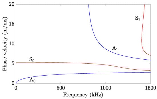
Figure 1.
Dispersion curve for a 2 mm aluminum plate evaluated with the Dispersion Calculator [70]. In the plotted frequency range, the two fundamental modes, as well as the first higher-order anti-symmetric (cut-off frequency around 800 kHz) and symmetric (cut-off frequency around 1400 kHz) modes are visible.
2.2. Frequency Domain Representation
In this section, an arbitrary time signal is considered, as illustrated in Figure 2. The Fourier transform of a real function shifted in time results in a complex, periodic function:
where , e denotes Euler’s number, , and . This relationship can be used to describe a wave measured by a sensor placed at a varying distance from the source [71] and is used in what follows to describe the scattering behavior of waves. As a comment, it should be mentioned that the Fourier transformation requires stationary signals.
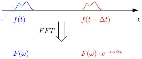
Figure 2.
Signal shifted in time and its periodic response in frequency domain.
2.3. Frequency Response Function (FRF) and Transmissibility Function
FRFs and transmissibility functions, which are well established in SHM [72], allow for evaluating a system’s response for various time history inputs. For the case of Lamb wave propagation investigated in this paper, both functions can be derived starting from the discretized form of the equilibrium equations of a Linear Time Invariant (LTI) Multi Degree of Freedom (MDOF) system:
where , , and describe the discretized mass, damping, and stiffness matrices, respectively, and vectors , , and denote the deformation vector and its first and second derivative with respect to time t. The right hand side of Equation (2) describes the excitation of the system, where denotes the spatial distribution of the excitation and its time history. This split of the excitation is possible, when the spatial distribution of the excitation is time invariant, which is usually the case for Lamb wave excitation [73]. Applying the Fourier transform to Equation (2), one obtains:
In the above, the same symbols are used for displacement and excitation f, regardless of whether they refer to frequency or time domain, since the corresponding domain is evident from their dependence on time or frequency, respectively.
Reorganizing Equation (3) yields the FRF [73]:
For discrete frequencies , the FRF can be evaluated numerically:
Dimilarly, if the FRF is available, the response for any given excitation can be computed as follows:
Next, the transmissibility function is derived for discrete frequencies from Equation (3). First, the equation is simplified by substituting :
Next, it is assumed that the response is known at a single Degree of Freedom (DOF) and should be calculated for all remaining locations. To this end, the system is partitioned in two sets of equations:
where subindex k refers to the DOF, where the response is known, and the subindex u to the unknown DOFs. This means and , where . Solving the second row of Equation (8) for and substituting in the first row yields the following:
Reorganizing Equation (9) and solving for the ratio of results in the definition of the transmissibility function [72]:
For discrete frequencies , the transmissibility function can be evaluated numerically:
while if the transmissibility function is available, the response for any given response at DOF k can be obtained as follows:
3. Method
The solver presented in this paper is based on the principle of ray tracing. Following this approach, each ray is represented by either discrete FRFs or discrete transmissibility functions—one function for each discrete frequency of interest. For each feature (e.g., defects or rivet holes) within the plate, several parameters need to be evaluated in an offline phase, which is described in Section 3.1, followed by a section on the use of these parameters in the online stage (Section 3.2). At this point, the following assumptions are put in place:
- The material is linear-elastic and isotropic.
- The features are assumed to be of circular shape, and therefore, the response is not affected by the direction of the incident wave.
- The size of the features is small compared to the size of the distances between actuator, sensors and features.
As the assumption of circular features introduces a strong limitation, it should be stated here that it is assumed that this assumption can be relaxed in future work. At this point, this assumption allows for training the Reduced Order Model (ROM) with very few simulations. A higher number of simulations is expected to allow the ROM to be trained for small features of any form.
3.1. Offline Phase
As a first step, the scattering behavior of an arbitrary feature is numerically investigated to extract the relevant information needed for the online phase. To extract this information, an idealized setup of an infinite plate with a single actuator, one feature, and one sensor (Figure 3) is chosen, where only a single mode is excited. In this setup, a direct wave packet from the actuator and one or several wave packets stemming from the feature can be measured at the sensor location. Several wave packets with their origin at the feature might be present, as mode conversion might occur at the feature—depending on the frequency and the feature’s shape.
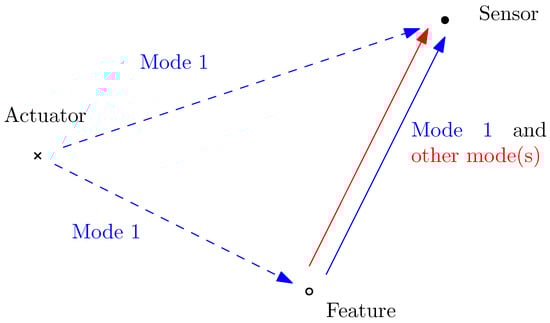
Figure 3.
Wave packets reaching a sensor with one scattering feature (e.g., a defect or a rivet hole): single mode actuation, several modes scattered at the feature. Dashed rays have their origin at the actuator, solid rays have their origin at the feature. No boundary reflections are considered at this point.
In what follows, we investigate the different wave packets, which reach a sensor, separately. Firstly, a baseline simulation is performed using the pristine setup, i.e., one without defects. Through baseline subtraction, the waves stemming from the feature can be extracted, given that the direct wave is known from the baseline. To differentiate between the different scattering waves from the feature, the deformations or internal forces on the cross section need to be investigated. Although this task is challenging in an experimental setting, it can be easily accomplished in simulation. Using this approach, all possible cases of wave packets propagating from the actuator to the feature and then to the sensor should be investigated. This means that in a setup where the two fundamental modes ( and ) are present and mode conversion occurs at the feature, four cases must be investigated. These cases are described by mode pairs, where the first mode is the one excited at the actuator and the second mode is the one investigated at the sensor: , , , and . Due to the linearity assumption, these cases can simply be superposed in a later step to obtain the full sensor response.
Next, several sensors are used in a radial line from the defect, as shown in Figure 4. The first sensor needs to have a certain distance from the feature to prevent evanescent waves from affecting the sensor response. A single mode wave packet, originating from the feature (due to either reflection of the same mode or mode conversion), changes its shape in between two sensors due to two effects, namely dispersion and geometric damping. Furthermore, the wave packets arrive later in time as the distance between sensor and feature grows. These three influences (dispersion, geometrical damping, time delay) on the sensor response are investigated next for discrete signals in frequency domain. Firstly, the geometric damping is known to be inversely proportional to [64,74], where d is the distance to the origin of the wave, and independent of the frequency. In contrast, dispersion is frequency-dependent and does not occur if the wave is composed of a single frequency. In the described method, the signal is separately investigated for each discrete frequency, implying that the dispersion is inherently accounted for, as it is a purely frequency-dependent phenomenon. As for the differentiation in terms of the time of arrival, it is shown in Section 2.2 that the response will be periodic. The time shift in Equation (1) thereby reflects the difference in distance . The relation between and is expressed as follows:
where is the frequency-dependent wave speed for the investigated mode and frequency ().
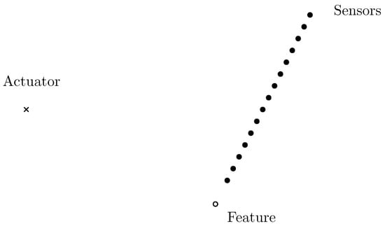
Figure 4.
A line of sensors in increasing distance from the defect (feature). The first sensor needs to be placed at a certain distance to the defect, as otherwise evanescent waves will occur, which distort the sensor response.
This means that the response at a sensor location for a discrete frequency and a certain mode can be described as follows:
with the unknown parameters being the amplitude A and phase shift . The frequency of the periodic term with respect to the distance can be evaluated, using the dispersion characteristics, as displayed in Figure 1. To avoid confusion, it should be emphasized at this point that is not a frequency with respect to time, but a spatial frequency with respect to the distance from the origin of the wave. In what follows, it is assumed that the sensor response along a radial line from a source can be adequately described by Equation (14).
Next, the amplitude A and phase shift need to be determined. With the amplitude A and the distance to the source d being strictly positive, the magnitude of the sensor response in Equation (14) becomes
And, therefore, as ,
The former implies that the amplitude could be extracted from a single sensor along the investigated radial line. However, within a practical setting, it is preferable to evaluate this for several virtual sensors and evaluate the mean so as to account for the fact that the size of the feature is small, but not 0. The only parameter that remains unknown is the phase , which can be inversely evaluated through use of an optimization scheme needing only a few sensors. For Section 4 of this paper, a Particle Swarm Optimization (PSO) employing eight virtual sensors showed satisfying results. As Equation (14) is expected to approximate the response at a sensor location for a discrete frequency well, the PSO determines with good approximation. At this point, it is possible to describe the response at various sensor locations along a line by only three parameters: the spatial frequency (), the amplitude (A), and the phase shift (). This allows for, firstly, significantly reducing the amount of stored training data and, secondly, accurately extrapolating beyond the distance of the last sensor used for training.
As the response along a radial line due to a specific excitation can be accurately described by Equation (14), it is of interest to obtain the response due to an arbitrary excitation. To achieve this, the concepts of Frequency Response Functions (FRFs) and transmissibility functions show promising results. These concepts, which are introduced in Section 2.3 and described by Equations (6) and (12), respectively, allow for evaluating the response in a sensor for inputs with different time-dependence. As stated above, the response for the sensors in Figure 4 due to the wave packets stemming from the feature is found through baseline subtraction. Following Equation (11), the transmissibility function for each sensor with respect to the baseline can be numerically evaluated as follows:
where the superscript denotes the baseline, describes the frequency response at the sensors, and the frequency response in the feature location. Similarly, for the case where the feature is present (denoted through the superscript ), it is calculated as follows:
For a feature of size 0, the frequency response at the feature is the same for the baseline and the case where the feature is present (). Therefore, the baseline subtracted transmissibility function (denoted through the superscript ) is found as follows:
This enables evaluating the response at each sensor location, if the excitation at the actuator location is different or if the distance between the actuator and the feature varies.
In a similar way, the response corresponding to a line of sensors that are radially placed with respect to the actuator can be compressed and simplified. The only difference to a wave packet stemming from a feature lies in the application of the principle of FRFs rather than the principle of transmissibility functions. In this case, in Equation (5) reflects the response at the sensors and the excitation at the actuator.
At this point, it is possible to evaluate the response for any sensor along the radial line from the feature by performing the following steps:
- Evaluate the response due to the direct wave:
- 1.1
- Evaluate the FRF for the distance from the actuator to the sensor;
- 1.2
- Multiply the obtained FRF with the excitation.
- Evaluate the virtual response at the feature:
- 2.1
- Evaluate the FRF for the distance from the actuator to the feature;
- 2.2
- Multiply the obtained FRF with the excitation.
- Evaluate the response for reflected and mode-converted wave packets:
- 3.1
- Evaluate the transmissibility functions for all modes of interest for the distance from the feature to the sensor;
- 3.2
- Multiply the obtained transmissibility functions with the response obtained in step 2.
- Sum up the response obtained in step 1.2 and the response obtained in step 3.2.
In what is described so far, each computed response corresponds to a sensor placed along a specific radial line. In order to more generally devise an approach to densely recover the response in the full field of an infinite, isotropic plate with a single feature, actuators along multiple radial lines can be employed covering a range of actuator–feature–sensor angles. The compression of each radial line of sensors into an amplitude (A) and a phase () proves advantageous in this respect. Using the same simulations that were previously used to infer the parameters (A and ) for a single line, an arbitrary number of lines can be compressed. Afterwards, the amplitude and the phase can be interpolated for each angle of interest. The limiting factors are the accuracy of the original simulation, the amount of data stored for the sensors, and the time needed for the optimization of the phase. These limitations do not hinder the evaluation and interpolation of a high number of parameters. Owing to the assumption of isotropic behavior, the evaluation for angles in the interval [0, π] is sufficient.
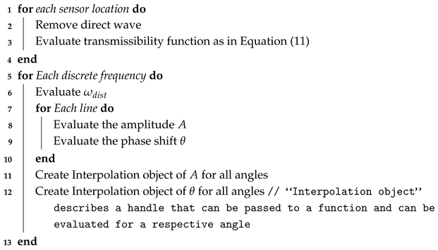
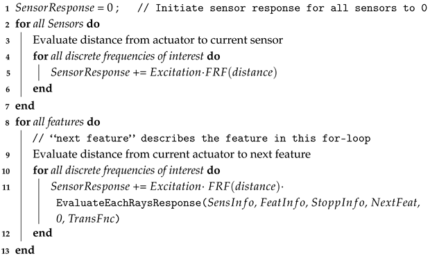
The offline process is summarized in Algorithm 1.
| Algorithm 1: Offline phase |
 |
3.2. Online Phase
The compressed FRFs and transmissibility functions can now be used to rapidly obtain the response at any plausible sensor location within a plate. For simplicity, in a first step, a scenario will be investigated where only a single wave mode is propagating, e.g., the –mode, in an infinite plate with two features and and a single sensor (Figure 5). Therefore, three points of interest exist to which a wave packet, excited at an actuator, will travel: the two feature and the sensor locations. We first investigate the wave from the actuator to the sensor. The response of the ray, representing this propagating wave packet, can be evaluated through the FRF determined in the offline part. Further, the two rays pointing from the actuator to the features need to be investigated, as these initiate reflections at the features. When further tracking the ray, which points to feature , reflections to two points of interest occur (dashed rays in Figure 5), where the first ray points to the sensor. To compute the sensor response of this path, three steps are necessary: (1) compute the FRF response of the ray pointing from the actuator to the feature ; (2) evaluate the transmissibility function for the ray pointing from the feature to the sensor; and (3) multiply this evaluated transmissibility function with evaluate FRF from step (1). The further reflection from the feature points to the feature , where reflections again occur at two points of interest: the sensor location and once again back in the feature position (dotted in Figure 5). The response at the sensor location can be evaluated by multiplying the FRF and the respective transmissibility function belonging to the respective ray on this path. This ray tracing can be understood as a tree, which is displayed in Figure 5b. In theory, the branches of this tree can be tracked to infinity; however, the amplitude reduces with every reflection and the cumulative length of relevant rays. Moreover, propagation across longer distances requires more time for the wave to arrive at the sensor, which is eventually longer than the investigated time period. Therefore, from a practical viewpoint, it is sufficient to investigate a finite number of reflections.
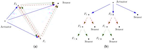
Figure 5.
An infinite plate comprising two features ( and , e.g., defects or rivet holes) and one sensor. Possible travel paths up to third order (meaning paths with up to three rays). Solid: first-order rays. Dashed: second-order rays. Dotted: third-order rays. (a) Possible travel paths. (b) Tree corresponding to the rays in (a).
Next, this concept should be generalized to a plate, where several modes occur. Therefore, a plate of infinite size comprising one actuator, one feature, and one sensor will be investigated, where the frequency of the excitation is chosen so that only the two fundamental modes ( and ) propagate, as displayed in Figure 6. As two modes might be excited, for each point of interest, two rays need to be investigated, one for each mode. The two possible modes entail the possibility of mode conversion at the feature. This leads to a total of four wave packets propagating from the feature to the sensor. These wave packets pertain to the reflected and mode-converted modes, stemming from the arriving mode, as well as the reflected and mode-converted modes, stemming from the arriving mode. At the sensor location, this leads to a total of six incoming wave packets, which need to be summed. These wave packets can be determined through the evaluated FRFs for the direct waves and the multiplication of the FRFs for the waves propagating to the feature, with the corresponding transmissibility functions for the reflected and mode-converted waves.
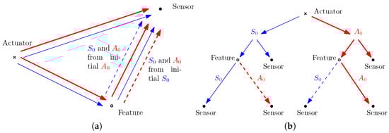
Figure 6.
An infinite plate with one feature and one sensor. Possible travel paths for propagating and modes. Thin lines: mode. Fat lines: mode. Dashed: and modes, stemming from mode conversion at the feature. (a) Possible travel paths. (b) Tree corresponding to the rays in (a).
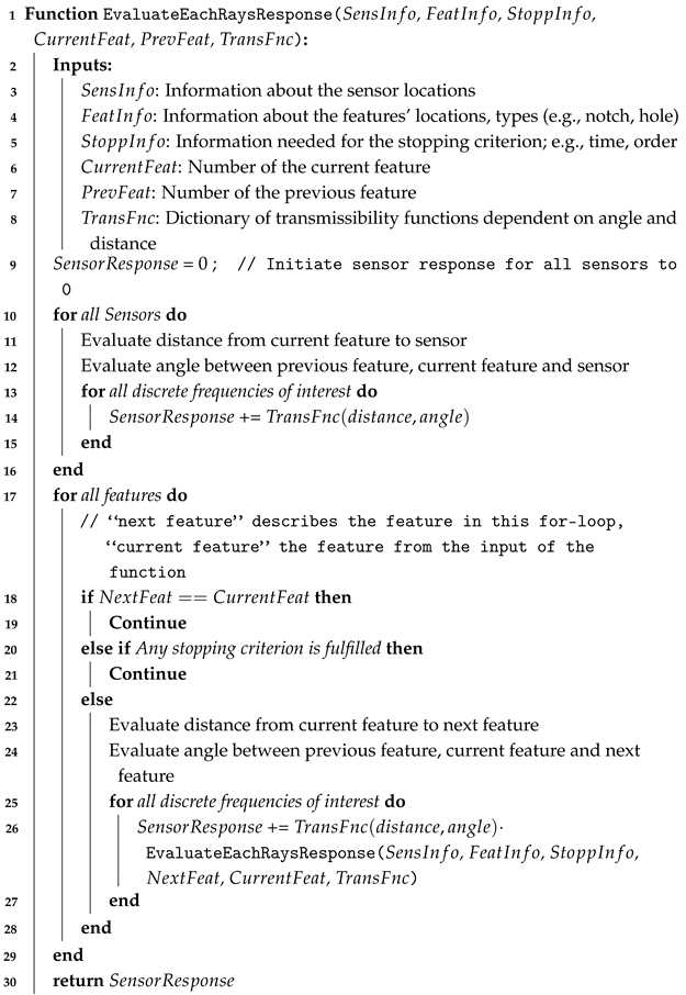
3.3. Algorithmic Implementation
As shown in Section 3.2, the ray tracing process can be represented as a tree structure. Within this tree structure, each feature can be seen as the start of a new tree, with nearly the same structure. This allows for implementing the algorithm in a recursive fashion, as outlined in Algorithm 2. The complete algorithm for the online part, including the first call of the recursive function, is displayed in Algorithm 3.
| Algorithm 2: Recursive function |
 |
| Algorithm 3: Online Phase |
 |
4. Results
The application of the described model to a synthetic example is described next. The performance of the surrogate is evaluated in terms of precision and speedup compared to the Full Order Models (FOMs).
4.1. Full Order Model (FOM)
To train the described surrogate and to evaluate its efficiency, high-fidelity simulations are necessary. Several spatial discretization methods are available for offering high-order Ansatz spaces that can effectively represent wave propagation according to Equation (2). See for instance the FEM with high polynomial degree (p-FEM) [75,76], the Scaled Boundary Finite Element Method (SBFEM) [77], or IsoGeometric Analysis (IGA) [78]. The Spectral Element Method (SEM) [79], which is also adopted in this work, is often one of the preferred alternatives due to its optimal mass lumping [80], rendering the use of fast explicit solvers (i.e., integrators in the time domain) straightforward.
Upon selecting an appropriate discretization method, an external meshing software, such as gmsh [81], can be used to model the domain. If a complex structure and/or various damage configurations are present, this can become a tedious and time-intensive task, which can render automatized damage-detection algorithms infeasible. With this, as well as other meshing-related issues, in mind, several enhancements of the aforementioned methods have been proposed, which enable supplementing the mesh with additional geometrical definitions, thus easing the reliance on the performance of meshing software.
In the present contribution, the SEM was supplemented with a mesh-independent representation of voids, whose influence on Equation (2) is accounted for via customized space integration rules. This approach, known as the Spectral Cell Method [82,83,84,85,86], allows for maintaining a level of efficiency that is on par with the SEM; however, it also leads to a loss of the diagonal mass matrix property for elements that are intersected by voids. To mitigate this issue, several alternatives have been proposed, including diagonal scaling [87], or moment fitting [88] schemes, as well as the use of implicit–explicit solvers [89,90]. In this contribution, we have adopted the latter approach, implemented in the C++ language. The corresponding code has been validated by comparison against a numerical implementation adopting shell elements [91], against benchmark analytical solutions for simple setups [88], as well as corroborated using Laser Doppler Vibrometer (LDV) experimental measurements [86].
4.2. Plate Configuration
For all given results, a 2 aluminum plate with its material properties displayed in Table 1 is examined. As previously described, a regular mesh is used for all simulations, with features modeled as voids via customized integration. Each element of the mesh is 3 mm × 3 mm × 2 mm with slightly smaller elements for sections whose dimensions are not a perfect multiple of 3 mm. Fourth-order spectral elements are utilized, and cut elements are described in [88].

Table 1.
Material properties.
To avoid boundary reflections, Absorbing Layers using Increasing Damping (ALID) are applied. The ALID scheme refers to several layers of elements at the boundary of the domain, with each layer comprising a higher damping coefficient as the distance from the plate increases, which allows for absorption of the incoming waves. Here, we apply ALID through 30 layers, each with a width of one element, and an increasing mass proportional damping. The damping coefficients are determined through a quadratic function, with the maximum damping coefficient assigned as 107 in the 30th layer, following the recommendations in [92].
4.3. Excitation
The excitation in the given examples stems from two point loads applied at the top and the bottom of the plate in different locations. This introduces some practical questions. If both loads comprise the same magnitude and are oriented to the same or opposite direction, the plate is, in theory, excited purely anti-symmetrically or symmetrically, respectively. However, it should be noted that even in a frequency range, where only the fundamental Lamb wave modes ( and ) are propagating, shear horizontal modes are activated. In the shown example, this introduces negligible error and is, therefore, ignored. If the shear horizontal modes are of interest, it should be possible to excite these in a targeted manner and consequently treat them similarly to Lamb wave modes. We acknowledge that point loads are not thoroughly depicting realistic excitation sources within an actual monitoring setup. In this initial example, we follow the assumption that the excitation source, the features and the sensors have quasi zero size. While this could be modeled for the excitation and sensors, this is not possible for the features, which need to be modeled with finite size. The features in the presented example are therefore modeled with non-zero size, which introduces errors. However, these errors are small, if the ratio between the size of the feature and the distance to the feature is small. For a non-point-wise excitation, the spatial dimension of the excitation will still be small compared to the size of the wave propagation distances and, therefore, non-point-wise excitations are also expected to be possible. When seeking to model arbitrary excitation sources, i.e., not symmetric or anti-symmetric, we can always express these via superposition of a symmetric and anti-symmetric counterpart, as the behavior of the plate is expected to be linear-elastic.
Two different excitation scenarios are applied. Firstly, in a training phase, a sudden impulse is applied as excitation, where the loading at the first time step is non-zero, while for all further time steps, the loading is zero. This is possible, as an impulse induces a broadband excitation across all discrete frequencies, thus allowing for the derivation of the FRFs and transmissibility functions for all frequencies of interest. For the testing phase, a Hann-window pulse is applied, as commonly used in SHM applications [13,28]. The Hann-window pulse is described as follows:
with denoting the carrier frequency of the pulse and c the number of cycles. A Hann-window excitation in frequency domain shows a narrow main lobe with flat side lobes. The frequency range covered by the main lobe can be evaluated through the following [93]:
A narrow and distinct frequency range allows for dealing with limited dispersion of the wave packet. For the following examples, the used Hann-windows will have a carrier frequency and cycles, resulting in a frequency range of interest between 180 and 420 . In this frequency range, the –mode is nearly non-dispersive, while the –mode is significantly dispersive (Figure 1).
4.4. Offline Phase
In the offline phase, the plate should be configured in order to learn the scattering behavior efficiently. The setup of the plate is shown in Figure 7, while the mesh details in the area of the features are illustrated in Figure 8. As two different features (a through hole with 5 mm radius and an elliptical notch with 5 mm radius and 0.5 mm depth) are investigated in what follows, a total of six simulations are needed. These simulations cover the three cases of a pristine plate, a plate with a through hole, and a plate with a notch, where for each case, a simulation with symmetric and anti-symmetric excitation, respectively, is needed. In total, 808 sensors are assumed to be the positions where the response is to be reconstructed by the delivered ROM. More specifically, we assume the sensor placed in an arrangement of 8 circles around the feature, with 101 sensors per circle.
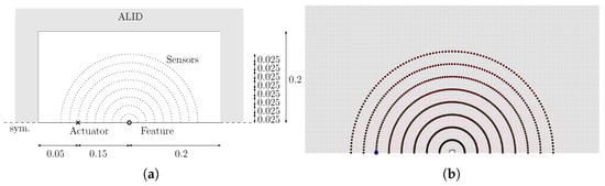
Figure 7.
Plate configuration for training. (a) Sketch of the plate, dimensions in [m]. (b) Mesh of the plate, with hole as a feature. Points are the sensor locations, and the large point marks the excitation. The size of the sensors is 0, and the feature has a radius of 5 mm.
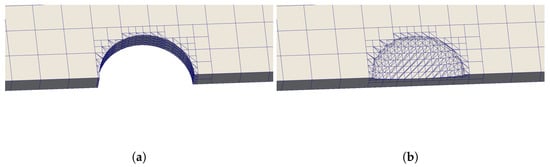
Figure 8.
Meshes of the plates, in the area of the features. (a) Mesh of the plate, in the area of the hole. (b) Mesh of the plate, in the area of the notch.
For these simulations, the time step size is set at , slightly less than the critical time step for the regular mesh. The simulations are run for 7999 time steps or a total of –. The total simulation time is chosen so that the slowest wave in the investigated frequency range reaches the outermost sensors. With these settings, a frequency step of 5 is achieved, where the first 160 discrete frequencies (up to 795 ) are investigated.
Based on these six simulations, a dictionary is formed. For each of the 101 radial directions and each of the 160 frequencies, a sine is fitted through the 8 radial points, with the phase found through a PSO. In a second step, the obtained amplitudes and phases are linearly interpolated through the circumference.
In Figure 9, Figure 10 and Figure 11, the scattering characteristics and accuracy of the created dictionary are assessed. Firstly, Figure 9 shows the scattering amplitude of the notch for different angles for the frequency of 400 . It is visible that for some angles, the scattering is very low. Figure 10 shows an instance of the FRF for an angle of 126° between the incident and the scattered wave. The decaying periodic function, described in Equation (14), is clearly visible. The surrogate accurately represents the behavior of the FOM, despite being trained only at 8 points along a line. Only for some points close to the notch, larger deviations can be observed. The error for individual training points can be seen in Figure 11. In comparison with Figure 9, it should be noticed that lines of high errors often correspond to angles of low amplitude and, therefore, a small denominator, when computing relative errors.
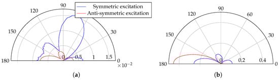
Figure 9.
Absolute value of the FRF at 400 kHz at a distance of 0.2 m to the notch for different angles. Incoming wave propagates from 0°. (a) Symmetric response. (b) Anti-symmetric response.
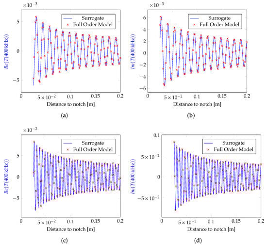
Figure 10.
Transmissibility function () along a line from a notch. The angle between the incident wave and the scattering line is 126° and the frequency is 400 kHz. (a) Real, symmetric response. (b) Imaginary, symmetric response. (c) Real, anti-symmetric response. (d) Imaginary, anti-symmetric response.
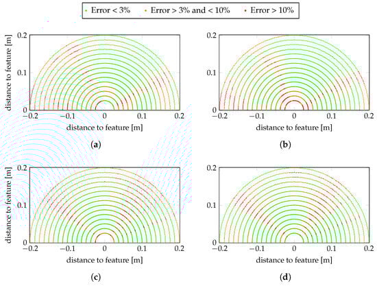
Figure 11.
Error for 400 kHz response for the notch in Figure 8b for symmetric excitation. The error for the real parts of each point is calculated as , where the subscript FOM refers to the FRF evaluated with the high-fidelity model, and the subscript ROM refers to the FRF evaluated with the surrogate. Incoming wave propagates from the right. (a) Error for the real part of the symmetric response. (b) Error for the imaginary part of the symmetric response. (c) Error for the real part of the anti-symmetric response. (d) Error for the imaginary part of the anti-symmetric response.
4.5. Online Phase
In Figure 12, a sketch of the plate configuration mesh used to test the online phase of the proposed approach is illustrated. This setup reflects a square plate with a single actuator, two features, and seven sensors. The origin of the coordinate system is assumed to coincide with the position of the actuator with a distance of to the left, to the right, and to the top and bottom boundary of the plate. The features are located at ( | ) and ( | ). Around the plate, there are 30 layers of ALID, to prevent boundary reflections.
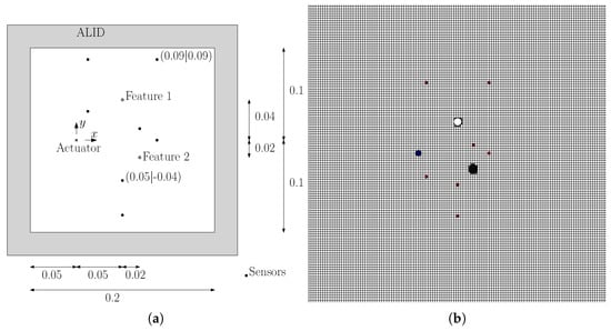
Figure 12.
Plate configuration for testing. (a) Sketch of the plate, dimensions in [m]. (b) Mesh of the plate, with hole as a Feature 1 and notch as Feature 2. Points are the sensor locations, and the large point marks the excitation.
We first examine the scenario where Feature 1 corresponds to a hole (as shown in Figure 8a) and Feature 2 is inactive. This means that a pure reflection without mode conversion is expected. Further, at most sensor locations, two wave packets are expected—the direct and the reflected wave packet—which may or may not overlap. For the sensor at location (0.09|0.09), the wave packet stemming from the feature is expected to result in a direction that is opposing the direct wave, as the sensor lies in the shadow of the feature. The plots for the sensors at locations (0.05|−0.04) and (0.09|0.09) are shown in Figure 13 and Figure 14, respectively.
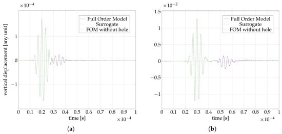
Figure 13.
Response at the sensor location (0.05|−0.04) for the case where Feature 1 is a hole and Feature 2 is inactive. (a) Symmetric excitation (error = ). (b) Anti-symmetric excitation (error = ).
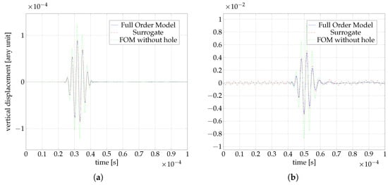
Figure 14.
Response at the sensor location (0.09|0.09) for the case where Feature 1 is a hole and Feature 2 is inactive. (a) Symmetric excitation (error = ). (b) Anti-symmetric excitation (error = ).
It can be seen in Figure 13, that there is an additional wave packet for both symmetric and anti-symmetric excitation, and that the additional wave packets are captured well by the surrogate, both in amplitude and in phase. For the sensor at location (0.09|0.09), which is placed in the shadow of the hole, it can be seen that the response without a hole would have a higher amplitude than for the case with a hole—an effect which is well captured by the surrogate. However, in the case of anti-symmetric excitation (Figure 14b), traces of a periodic signal are discernible in the response of the surrogate. These are artifacts, which likely result from a poorly fitted frequency for a certain angle. This seems tolerable, as the overall response is fitted well.
Next, in Figure 15 and Figure 16, the response is displayed for the case where Feature 1 is a notch rather than a hole. Figure 15a allows for clearly distinguishing three arriving wave packets, compared to the two which were visible in the case of the hole (Figure 13a). Therefore, the additional, third wave packet stems from mode conversion from the incident symmetric wave packet into an anti-symmetric wave packet. Further, it can be seen that the amplitude of the reflected symmetric wave packet is smaller in this case, since the notch only reduces the cross section, while the hole goes through the whole cross section. On the other hand, the reduction in the cross section results in a minor drop in the amplitude of the direct wave for the case of the sensor being in the shadow of the feature (Figure 15) compared to the case with the hole. All these effects are captured well by the surrogate. For the sensor located in location (0.09|0.09), the wave packets originating from the notch are hardly distinguishable from the direct wave (Figure 16a). However, the surrogate still matches the behavior predicted by the FOM well. Although the effect of the notch is clearly visible for the case of symmetric excitation, there is hardly any effect for the case of the anti-symmetric excitation. This is expected due to the high difference in the amplitude for symmetric and anti-symmetric modes for the out-of-plane displacement (here approximately two orders of magnitude).
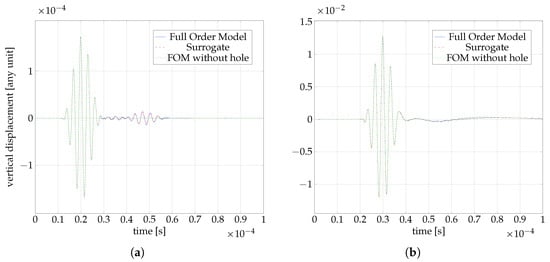
Figure 15.
Response at the sensor location (0.05|−0.04) for the case where Feature 1 is a notch and Feature 2 is inactive. (a) Symmetric excitation (error = ). (b) Anti-symmetric excitation (error = ).
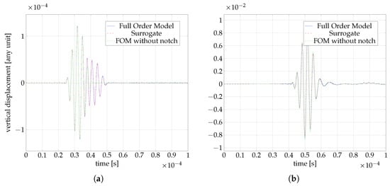
Figure 16.
Response at the sensor location (0.09|0.09) for the case where Feature 1 is a notch and Feature 2 is inactive. (a) Symmetric excitation (error = ). (b) Anti-symmetric excitation (error = ).
For the plots in Figure 17, both features are modeled as holes. Focusing on the case of anti-symmetric excitation in Figure 17b, four wave packets are now visible. The first wave packet stems from the direct wave, while the second and third wave packets correspond to the reflections from the two holes. The fourth wave packet stems from a wave path, which includes reflections at both holes (i.e., Actuator–Feature 1–Feature 2–Sensor or Actuator–Feature 2–Feature 1–Sensor), while the wave packet from the other path that includes both wave packets is not clearly visible. This may be attributed to an overlap with one of the other wave packets or to the amplitude for this path dropping significantly, to the point that it is not visibly discernible. Finally, the results for the case where Feature 1 corresponds to a hole and Feature 2 is a notch can be seen in Figure 18, where, again, the main wave packets are captured in amplitude and phase. The additional sensor locations marked in Figure 12, including those within the defect region, showed similar accuracy to the results presented in the presented plots.
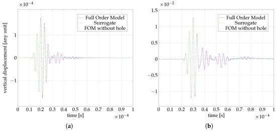
Figure 17.
Response at the sensor location (0.05|−0.04) for the case where Feature 1 is a hole and Feature 2 is a hole. (a) Symmetric excitation (error = ). (b) Anti-symmetric excitation (error = ).
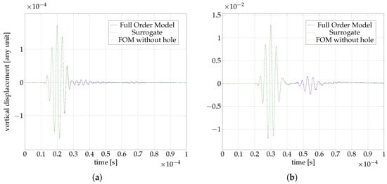
Figure 18.
Response at the sensor location (0.05|−0.04) for the case where Feature 1 is a hole and Feature 2 is a notch. (a) Symmetric excitation (error = ). (b) Anti-symmetric excitation (error = ).
4.6. Speedup
All surrogate simulations were performed on a single Intel(R) Xeon(R) Gold 5318Y CPU @ core using Matlab 2024a [94], while the FOM simulations were run on the ETH Euler cluster with eight core AMD EPYC 7742 processors (2.25 GHz nominal, peak of 3.4 GHz). The surrogate simulations with a single feature take approximately and with two features approximately for the seven sensors displayed in Figure 12. On the other hand, the computational time for the FOM is nearly independent of the features, corresponding to for each simulation. For the cases considered and when using the described hardware, this results in a speedup in the order of 103 to 104. In addition, tests including three and four features were performed, where the simulations were run for approximately 16 and 49 , respectively, resulting in a speedup in the order of 102. Generally, the computational time for the surrogate depends heavily on the number of features that are assumed to be present, but only indirectly depends on the size of the plate (through the attenuation and the propagation time). Conversely, computing the FOM is heavily dependent on the size of the plate, while the effect of the features on the numerical toll is only minor, albeit implying a required mesh modification.
5. Discussion
We introduce an approach to efficiently model guided wave-based sensing scenarios by delivering a surrogate for rapid evaluation of Lamb wave propagation. The method can flexibly account for diverse geometrical features and is easily extendable to more complex setups. In this study, which serves more as an introduction to the approach, we place the following specific assumptions:
- The plate is assumed to be composed of a linear-elastic and isotropic material.
- The area where the excitation is applied, the features, and the sensors are considered small compared to their interconnecting distance and can, therefore, be assumed to be point-wise.
- The explored frequency range is chosen so that only fundamental modes are propagating and only the out-of-plane displacement is investigated.
- No viscous damping is assumed.
Most of these assumptions can be relaxed, while others are allowed for the usual cases explored within the Non-Destructive Evaluation (NDE) and SHM contexts, given the small amplitude of actuated Lamb waves. The method introduces a new approach to modeling GW-based assessment, featuring the following advantages:
- The computational cost of the surrogate is significantly lower to the FOMs and therefore suited for inverse problem settings, as mandated in condition monitoring and damage diagnosis tasks. In the provided examples, the speedup is in the order of 103 to 104.
- The method can be extended to account for further intricacies, including geometries that accommodate diversified plate setups. The authors expect that an extension to anisotropic plates is possible with more training simulations.
- The full time history at the sensor location is reconstructed, and not only the arrival time or the amplitude, as furnished by commonly adopted alternatives.
- The mechanics behind the surrogate is well understood.
Rooting the method in mechanics principles reduces the training effort, with only few simulations required for training, while ensuring that the model estimates can be extrapolated. Furthermore, the process allows for tracking single wave packets through various possible propagation paths, which allows gaining information on the individual wave packets present in the sensor response. This allows a better understanding of the wave propagation phenomena, which is superior compared to the classical FOMs.
Building on the proposed method, several promising avenues for further research can be explored. While the current approach focuses on circular defects, a modified training strategy could enable its application to more complex geometries, significantly expanding its versatility. To further enhance efficiency, investigating the relationship between scattering wave characteristics and defect size could reduce the need for extensive training simulations. Notably, Diligent et al. [64] observed that for holes, the amplitude of scattering waves is nearly proportional to their diameter—an insight that could be leveraged to refine the model. For real-world applications, incorporating boundary reflections is essential. A key step in this direction is analyzing the interaction between different wave modes at the boundary, such as shear horizontal and anti-symmetric modes [52]. Additionally, extending the method to anisotropic materials presents an exciting opportunity to account for direction-dependent wave propagation speeds, further broadening its applicability. Optimizing sensor placement also holds great potential. While the current offline approach employs a regular grid, a strategically optimized placement could minimize errors, as observed in Figure 14b. Finally, enhancing computational efficiency through parallelization and adaptive stopping strategies would further accelerate the surrogate model, making it even more effective for practical use.
Author Contributions
Conceptualization, P.S., E.C. and K.A.; methodology, P.S., E.C. and K.A.; software, P.S.; validation, P.S. and K.A.; formal analysis, P.S.; investigation, P.S.; writing—original draft preparation, P.S., E.C. and K.A.; writing—review and editing, P.S., R.S., W.O., E.C. and K.A.; visualization, P.S.; supervision, E.C. and K.A.; project administration, E.C.; funding acquisition, W.O. and E.C. All authors have read and agreed to the published version of the manuscript.
Funding
This research is conducted as part of the project “Fusion of Models and Data for Enriched Evaluation of Structural Health” financed by the National Science Center (Poland) and the Swiss National Science Foundation (200021L_192139). The authors also wish to acknowledge the MSCA Staff Exchanges 2021 project ReCharged (Grant ID: 101086413). This project has received funding 505 from the Horizon Europe Programme under the Marie Skłodowska-Curie Staff Exchanges Action (GA no. 101086413), co-funded by the UK Research & Innovation and the Swiss State Secretariat for Education, Research & Innovation. Dr Rohan Soman acknowledges the support of the COST Action HISTRATE CA21155.
Informed Consent Statement
Not applicable.
Data Availability Statement
No new data were created or analyzed in this study. Data sharing is not applicable to this article.
Conflicts of Interest
The authors declare no conflicts of interest.
Abbreviations
The following abbreviations are used in this manuscript:
| ALID | Absorbing Layers using Increasing Damping |
| CFRP | Carbon Fiber Reinforced Polymer |
| CMEP | Complex Modes Expansion with vector Projection |
| CNN | Convolutional Neural Network |
| DAS | Delay-And-Sum |
| DNN | Dense Neural Network |
| DL | Deep Learning |
| DOF | Degree of Freedom |
| DOFs | Degrees of Freedom |
| DORT-MUSIC | Decomposition of the Time-Reversal Operator and MUltiple SIgnal Classification |
| FCM | Finite Cell Method |
| FEM | Finite element method |
| FOM | Full Order Model |
| FRF | Frequency Response Function |
| FWI | Full Waveform Inversion |
| IGA | IsoGeometric Analysis |
| LDV | Laser Doppler Vibrometer |
| LSTM | Long Short-Term Memory |
| LTI | Linear Time Invariant |
| MDOF | Multi Degree of Freedom |
| MOR | Model Order Reduction |
| NDE | Non-Destructive Evaluation |
| p-FEM | FEM with high polynomial degree |
| PGD | Proper Generalized Decomposition |
| PSO | Particle Swarm Optimization |
| RNN | Recurrent Neural Network |
| ROM | Reduced Order Model |
| SBFEM | Scaled Boundary Finite Element Method |
| SDP | Scattering Directivity Pattern |
| SEM | Spectral Element Method |
| SFEM | Spectral Finite Element Method |
| SHM | Structural Health Monitoring |
| SR | Sparse Reconstruction |
| SVD | Singular Value Decomposition |
| ToF | Time of Flight |
| TRM | Time-Reversal Method |
| WFI | Waveform Feature Index |
References
- Lamb, H. On waves in an elastic plate. Proc. R. Soc. Lond. Ser. A Contain. Pap. Math. Phys. Character 1917, 93, 114–128. [Google Scholar] [CrossRef]
- Shao, Y.; Zeng, L.; Lin, J. Damage detection of thick plates using trailing pulses at large frequency-thickness products. Appl. Acoust. 2021, 174, 107767. [Google Scholar] [CrossRef]
- Mitra, M.; Gopalakrishnan, S. Guided wave based structural health monitoring: A review. Smart Mater. Struct. 2016, 25, 053001. [Google Scholar] [CrossRef]
- He, M.; Dong, C.; Sun, X.; He, J. Fatigue Crack Monitoring Method Based on the Lamb Wave Damage Index. Materials 2024, 17, 3836. [Google Scholar] [CrossRef]
- Sieber, P.; Kudela, P.; Soman, R.; Chatzi, E. Wind turbine blade structural health monitoring dataset. 2024. [Google Scholar] [CrossRef]
- Soleimanpour, R.; Ng, C.T. Scattering of the fundamental anti-symmetric Lamb wave at through-thickness notches in isotropic plates. J. Civ. Struct. Health Monit. 2016, 6, 447–459. [Google Scholar] [CrossRef]
- Capineri, L.; Taddei, L.; Marino Merlo, E. Detection of a Submillimeter Notch-Type Defect at Multiple Orientations by a Lamb Wave A0 Mode at 550 kHz for Long-Range Structural Health Monitoring Applications. Sensors 2024, 24, 1926. [Google Scholar] [CrossRef] [PubMed]
- Yelve, N.P.; Mitra, M.; Mujumdar, P. Detection of delamination in composite laminates using Lamb wave based nonlinear method. Compos. Struct. 2017, 159, 257–266. [Google Scholar] [CrossRef]
- Soleimanpour, R.; Ng, C.T. Locating delaminations in laminated composite beams using nonlinear guided waves. Eng. Struct. 2017, 131, 207–219. [Google Scholar] [CrossRef]
- Nicard, C.; Rébillat, M.; Devos, O.; El May, M.; Letellier, F.; Dubent, S.; Thomachot, M.; Fournier, M.; Masse, P.; Mechbal, N. In-situ monitoring of µm-sized electrochemically generated corrosion pits using Lamb waves managed by a sparse array of piezoelectric transducers. Ultrasonics 2025, 147, 107527. [Google Scholar] [CrossRef]
- Gorgin, R.; Luo, Y.; Wu, Z. Environmental and operational conditions effects on Lamb wave based structural health monitoring systems: A review. Ultrasonics 2020, 105, 106114. [Google Scholar] [CrossRef] [PubMed]
- Ismail, N.; Hafizi, Z.M.; Lim, K.S.; Ahmad, H. Lamb Wave Actuation Techniques for SHM System—A Review. In Technological Advancement in Instrumentation & Human Engineering; Hassan, M.H.A., Zohari, M.H., Kadirgama, K., Mohamed, N.A.N., Aziz, A., Eds.; Springer Nature: Singapore, 2023; pp. 677–685. [Google Scholar]
- Zhou, K.; Zhou, Z.; Yang, Z.; Xu, X.; Wu, Z. Axisymmetric and non-axisymmetric Lamb wave excitation using rectangular actuators. Smart Mater. Struct. 2019, 28, 115024. [Google Scholar] [CrossRef]
- Seher, M.; Huthwaite, P.; Lowe, M.J.; Nagy, P.B. Model-based design of low frequency Lamb wave EMATs for mode selectivity. J. Nondestruct. Eval. 2015, 34, 22. [Google Scholar] [CrossRef]
- Michaels, J.E. Detection, localization and characterization of damage in plates with an in situ array of spatially distributed ultrasonic sensors. Smart Mater. Struct. 2008, 17, 035035. [Google Scholar] [CrossRef]
- Sharif-Khodaei, Z.; Aliabadi, M.H. Assessment of delay-and-sum algorithms for damage detection in aluminium and composite plates. Smart Mater. Struct. 2014, 23, 075007. [Google Scholar] [CrossRef]
- Kulakovskyi, A.; Mesnil, O.; Chapuis, B.; d’Almeida, O.; Lhémery, A. Statistical Analysis of Guided Wave Imaging Algorithms Performance Illustrated by a Simple Structural Health Monitoring Configuration. J. Nondestruct. Eval. Diagn. Progn. Eng. Syst. 2021, 4, 031001. [Google Scholar] [CrossRef]
- Levine, R.M. Ultrasonic Guided Wave Imaging via Sparse Reconstruction. Ph.D. Thesis, Georgia Institute of Technology, Atlanta, GA, USA, 2014. [Google Scholar]
- Nokhbatolfoghahai, A.; Navazi, H.M.; Groves, R.M. Use of delay and sum for sparse reconstruction improvement for structural health monitoring. J. Intell. Mater. Syst. Struct. 2019, 30, 2919–2931. [Google Scholar] [CrossRef]
- Watkins, R.; Jha, R. A modified time reversal method for Lamb wave based diagnostics of composite structures. Mech. Syst. Signal Process. 2012, 31, 345–354. [Google Scholar] [CrossRef]
- Dai, D.; He, Q. Structure damage localization with ultrasonic guided waves based on a time–frequency method. Signal Process. 2014, 96, 21–28. [Google Scholar] [CrossRef]
- Cantero-Chinchilla, S.; Chiachío, J.; Chiachío, M.; Chronopoulos, D.; Jones, A. A robust Bayesian methodology for damage localization in plate-like structures using ultrasonic guided-waves. Mech. Syst. Signal Process. 2019, 122, 192–205. [Google Scholar] [CrossRef]
- Rautela, M.; Gopalakrishnan, S. Deep learning frameworks for wave propagation-based damage detection in 1d-waveguides. In Proceedings of the 11th International Symposium on NDT in Aerospace, Paris, France, 13–15 November 2019; Volume 2, pp. 1–11. [Google Scholar]
- Azadi, S.; Okabe, Y.; Carvelli, V. Bayesian-optimized 1D-CNN for delamination classification in CFRP laminates using raw ultrasonic guided waves. Compos. Sci. Technol. 2025, 264, 111101. [Google Scholar] [CrossRef]
- Rautela, M.; Senthilnath, J.; Moll, J.; Gopalakrishnan, S. Combined two-level damage identification strategy using ultrasonic guided waves and physical knowledge assisted machine learning. Ultrasonics 2021, 115, 106451. [Google Scholar] [CrossRef] [PubMed]
- Postorino, H.; Monteiro, E.; Rébillat, M.; Mechbal, N. Cross-structures deep transfer learning through kantorovich potentials for lamb waves based structural health monitoring. J. Struct. Dyn. 2023, 2, 24–50. [Google Scholar] [CrossRef]
- Sun, Y.; Xu, Y.; Li, W.; Li, Q.; Ding, X.; Huang, W. A Lamb Waves Based Ultrasonic System for the Simultaneous Data Communication, Defect Inspection, and Power Transmission. IEEE Trans. Ultrason. Ferroelectr. Freq. Control 2021, 68, 3192–3203. [Google Scholar] [CrossRef]
- Wang, J.; Shen, Y. An enhanced Lamb wave virtual time reversal technique for damage detection with transducer transfer function compensation. Smart Mater. Struct. 2019, 28, 085017. [Google Scholar] [CrossRef]
- He, J.; Yuan, F.G. Lamb wave-based subwavelength damage imaging using the DORT-MUSIC technique in metallic plates. Struct. Health Monit. 2016, 15, 65–80. [Google Scholar] [CrossRef]
- Fan, S.; Zhang, A.; Sun, H.; Yun, F. A Local TR-MUSIC Algorithm for Damage Imaging of Aircraft Structures. Sensors 2021, 21, 3334. [Google Scholar] [CrossRef] [PubMed]
- An, Y.; Pang, C.; Cui, R.; Ou, J. Debonding damage detection in CFRP-reinforced steel structures using scanning probabilistic imaging method improved by ultrasonic guided-wave transfer function. Ultrasonics 2025, 149, 107592. [Google Scholar] [CrossRef]
- Yang, Z.B.; Zhu, M.F.; Lang, Y.F.; Chen, X.F. Estimation of Lamb wave propagation by means of Fourier spectral frequency response function. Nondestruct. Test. Eval. 2022, 37, 160–183. [Google Scholar] [CrossRef]
- Kudela, P.; Radzienski, M.; Ostachowicz, W.; Yang, Z. Structural Health Monitoring system based on a concept of Lamb wave focusing by the piezoelectric array. Mech. Syst. Signal Process. 2018, 108, 21–32. [Google Scholar] [CrossRef]
- Yang, Z.B.; Zhu, M.F.; Lang, Y.F.; Chen, X.F. FRF-based lamb wave phased array. Mech. Syst. Signal Process. 2022, 166, 108462. [Google Scholar] [CrossRef]
- Zhou, W.; Ichchou, M. Wave propagation in mechanical waveguide with curved members using wave finite element solution. Comput. Methods Appl. Mech. Eng. 2010, 199, 2099–2109. [Google Scholar] [CrossRef]
- Ahmed, A.; Din, I.U.; Kulkarni, S.; Khan, K.A. Multiscale finite element modeling of origami-inspired dual matrix deployable composite with visco-hyperelastic hinge. Compos. Struct. 2024, 343, 118301. [Google Scholar] [CrossRef]
- Bürchner, T.; Kopp, P.; Kollmannsberger, S.; Rank, E. Immersed boundary parametrizations for full waveform inversion. Comput. Methods Appl. Mech. Eng. 2023, 406, 115893. [Google Scholar] [CrossRef]
- Rabinovich, D.; Givoli, D.; Turkel, E. Single-field identification of inclusions and cavities in an elastic medium. Int. J. Numer. Methods Eng. 2024, 125, e7364. [Google Scholar] [CrossRef]
- Bürchner, T.; Kopp, P.; Kollmannsberger, S.; Rank, E. Isogeometric multi-resolution full waveform inversion based on the finite cell method. Comput. Methods Appl. Mech. Eng. 2023, 417, 116286. [Google Scholar] [CrossRef]
- Zakian, P.; Nadi, M.; Tohidi, M. Finite cell method for detection of flaws in plate structures using dynamic responses. Structures 2021, 34, 327–338. [Google Scholar] [CrossRef]
- Rautela, M.; Gopalakrishnan, S. Ultrasonic guided wave based structural damage detection and localization using model assisted convolutional and recurrent neural networks. Expert Syst. Appl. 2021, 167, 114189. [Google Scholar] [CrossRef]
- Benner, P.; Gugercin, S.; Willcox, K. A survey of projection-based model reduction methods for parametric dynamical systems. SIAM Rev. 2015, 57, 483–531. [Google Scholar] [CrossRef]
- Greif, C.; Urban, K. Decay of the Kolmogorov N-width for wave problems. Appl. Math. Lett. 2019, 96, 216–222. [Google Scholar] [CrossRef]
- Amsallem, D.; Zahr, M.J.; Farhat, C. Nonlinear model order reduction based on local reduced-order bases. Int. J. Numer. Methods Eng. 2012, 92, 891–916. [Google Scholar] [CrossRef]
- Bigoni, C. Numerical Methods for Structural Anomaly Detection Using Model Order Reduction and Data-Driven Techniques. Ph.D. Thesis, EPFL, Lausanne, Switzerland, 2020. [Google Scholar] [CrossRef]
- Bigoni, C.; Guo, M.; Hesthaven, J.S. Predictive Monitoring of Large-Scale Engineering Assets Using Machine Learning Techniques and Reduced-Order Modeling. In Structural Health Monitoring Based on Data Science Techniques; Cury, A., Ribeiro, D., Ubertini, F., Todd, M.D., Eds.; Springer International Publishing: Cham, Switzerland, 2022; pp. 185–205. [Google Scholar] [CrossRef]
- Sieber, P.; Agathos, K.; Soman, R.; Ostachowicz, W.; Chatzi, E. Guided Wave–Based Defect Localization via Parameterized FRF-Based Reduced-Order Models. J. Eng. Mech. 2024, 150, 04024059. [Google Scholar] [CrossRef]
- Goutaudier, D.; Berthe, L.; Chinesta, F. Proper Generalized Decomposition with time adaptive space separation for transient wave propagation problems in separable domains. Comput. Methods Appl. Mech. Eng. 2021, 380, 113755. [Google Scholar] [CrossRef]
- Yan, W.J.; Chronopoulos, D.; Papadimitriou, C.; Cantero-Chinchilla, S.; Zhu, G.S. Bayesian inference for damage identification based on analytical probabilistic model of scattering coefficient estimators and ultrafast wave scattering simulation scheme. J. Sound Vib. 2020, 468, 115083. [Google Scholar] [CrossRef]
- Drakoulas, G.; Gortsas, T.; Polyzos, D. Physics-based reduced order modeling for uncertainty quantification of guided wave propagation using Bayesian optimization. Eng. Appl. Artif. Intell. 2024, 133, 108531. [Google Scholar] [CrossRef]
- Postorino, H.; Rebillat, M.; Monteiro, E.; Mechbal, N. Towards an Industrial Deployment of PZT Based SHM Processes: A Dedicated Metamodel for Lamb Wave Propagation. In European Workshop on Structural Health Monitoring; Rizzo, P., Milazzo, A., Eds.; Springer International Publishing: Cham, Switzerland, 2021; pp. 720–731. [Google Scholar]
- Barras, J.; Lhémery, A.; Impériale, A. Modal pencil method for the radiation of guided wave fields in finite isotropic plates validated by a transient spectral finite element method. Ultrasonics 2020, 103, 106078. [Google Scholar] [CrossRef]
- Barras, J.; Lhémery, A. Modal pencil method for the radiation of guided wave fields in composite plates of finite size. NDT E Int. 2022, 126, 102598. [Google Scholar] [CrossRef]
- Mardanshani, A.; Van Den Abeele, K.; Chronopoulus, D. Semi-analytical simulation of ultrasound wave propagation in large plate-like structures. In Proceedings of the European Workshop on Structural Health Monitoring, Potsdam, Germany, 10–13 June 2024; pp. 10–13. [Google Scholar]
- Xu, C.; Yang, Z.; Deng, M. Weighted Structured Sparse Reconstruction-Based Lamb Wave Imaging Exploiting Multipath Edge Reflections in an Isotropic Plate. Sensors 2020, 20, 3502. [Google Scholar] [CrossRef]
- Allouko, A.; Bonnet-Ben Dhia, A.S.; Lhémery, A.; Baronian, V. Optimal computation of integrals in the Half-Space Matching method for modal simulation of SHM/NDE in 3D elastic plate. J. Phys. Conf. Ser. 2024, 2768, 012004. [Google Scholar] [CrossRef]
- Lozano, D.; Bulling, J.; Gravenkamp, H.; Birk, C. Domain decoupling implementation for efficient ultrasonic wave simulations using scaled boundary finite elements and the mortar method. Comput. Methods Appl. Mech. Eng. 2023, 417, 116465. [Google Scholar] [CrossRef]
- Briand, W.; Rébillat, M.; Guskov, M.; Mechbal, N. Damage size quantification using lamb waves by analytical model identification. In European Workshop on Structural Health Monitoring; Springer: Cham, Switzerland, 2022; pp. 119–127. [Google Scholar]
- Poddar, B.; Giurgiutiu, V. Fast and accurate analytical model to solve inverse problem in SHM using Lamb wave propagation. In Nondestructive Characterization and Monitoring of Advanced Materials, Aerospace, and Civil Infrastructure 2016; Yu, T., Gyekenyesi, A.L., Shull, P.J., Wu, H.F., Eds.; International Society for Optics and Photonics, SPIE: Bellingham, WA, USA, 2016; Volume 9804, p. 98041J. [Google Scholar] [CrossRef]
- Soleimanpour, R.; Soleimani, S.M. Scattering analysis of linear and nonlinear symmetric Lamb wave at cracks in plates. Nondestruct. Test. Eval. 2022, 37, 439–463. [Google Scholar] [CrossRef]
- Sedaghati, A.; Honarvar, F.; Tabatabaeipour, M.; Sinclair, A.N. Investigation of the scattering of Lamb waves from a generalized circular cavity by using Poisson/Mindlin plate theories and numerical simulation. Proc. Inst. Mech. Eng. Part C J. Mech. Eng. Sci. 2020, 234, 152–170. [Google Scholar] [CrossRef]
- Fromme, P.; Rouge, C. Directivity of guided ultrasonic wave scattering at notches and cracks. J. Phys. Conf. Ser. 2011, 269, 012018. [Google Scholar] [CrossRef]
- Golub, M.V.; Shpak, A.N.; Mueller, I.; Fomenko, S.I.; Fritzen, C.P. Lamb Wave Scattering Analysis for Interface Damage Detection between a Surface-Mounted Block and Elastic Plate. Sensors 2021, 21, 860. [Google Scholar] [CrossRef]
- Diligent, O.; Grahn, T.; Boström, A.; Cawley, P.; Lowe, M.J.S. The low-frequency reflection and scattering of the S0 Lamb mode from a circular through-thickness hole in a plate: Finite Element, analytical and experimental studies. J. Acoust. Soc. Am. 2002, 112, 2589–2601. [Google Scholar] [CrossRef] [PubMed]
- Ostachowicz, W.; Kudela, P.; Krawczuk, M.; Zak, A. Introduction to the Theory of Elastic Waves. In Guided Waves in Structures for SHM; John Wiley & Sons, Ltd.: Hoboken, NJ, USA, 2012; Chapter 1; pp. 1–46. [Google Scholar] [CrossRef]
- Giurgiutiu, V. Chapter 6 - Guided Waves. In Structural Health Monitoring with Piezoelectric Wafer Active Sensors, 2nd ed.; Giurgiutiu, V., Ed.; Academic Press: Oxford, UK, 2014; pp. 293–355. [Google Scholar] [CrossRef]
- Rodriguez, S.; Rébillat, M.; Paunikar, S.; Margerit, P.; Monteiro, E.; Chinesta, F.; Mechbal, N. Single atom convolutional matching pursuit: Theoretical framework and application to Lamb waves based structural health monitoring. Signal Process. 2025, 231, 109898. [Google Scholar] [CrossRef]
- Imano, K.; Endo, T. Experimental Study on the Mode Conversion of Lamb Wave Using a Metal Plate Having a Notch Type Defect. Int. J. Soc. Mater. Eng. Resour. 2013, 19, 20–23. [Google Scholar] [CrossRef]
- Galán, J.M.; Abascal, R. Lamb mode conversion at edges. A hybrid boundary element–finite-element solution. J. Acoust. Soc. Am. 2005, 117, 1777–1784. [Google Scholar] [CrossRef]
- Huber, A. ArminHuber/Dispersion-Calculator: Dispersion Calculator v3.0. 2024. Available online: https://zenodo.org/records/14167846 (accessed on 20 March 2015).
- Sieber, P.; Agathos, K.; Soman, R.; Ostachowicz, W.; Chatzi, E. Towards a FRF-based parametric surrogate for guided wave-based evaluation in multiple defect scenarios. In Health Monitoring of Structural and Biological Systems XVIII; Su, Z., Peters, K.J., Ricci, F., Rizzo, P., Eds.; International Society for Optics and Photonics, SPIE: Bellingham, WA, USA, 2024; Volume 12951, p. 129510C. [Google Scholar] [CrossRef]
- Chesné, S.; Deraemaeker, A. Damage localization using transmissibility functions: A critical review. Mech. Syst. Signal Process. 2013, 38, 569–584. [Google Scholar] [CrossRef]
- Sieber, P.; Agathos, K.; Soman, R.; Ostachowicz, W.; Chatzi, E. A parametrized Reduced Order Model for rapid evaluation of flaws in Guided Wave testing. In Structural Health Monitoring 2021: Enabling Next Generation SHM for Cyber-Physical Systems; DEStech Publications: Lancaster, PA, USA, 2022; pp. 679–686. [Google Scholar]
- Hall, L. Simulations and Analyses of Train-Induced Ground Vibrations: A Comparative Study of Two-and Three-Dimensional Calculations with Actual Measurements. Ph.D. Thesis, Royal Institute of Technology, Stockholm, Sweden, 2000. [Google Scholar]
- Willberg, C.; Duczek, S.; Vivar Perez, J.; Schmicker, D.; Gabbert, U. Comparison of different higher order finite element schemes for the simulation of Lamb waves. Comput. Methods Appl. Mech. Eng. 2012, 241–244, 246–261. [Google Scholar] [CrossRef]
- Düster, A.; Rank, E.; Szabó, B. The-Version of the Finite Element and Finite Cell Methods. In Encyclopedia of Computational Mechanics, 2nd ed.; John Wiley & Sons, Ltd.: Hoboken, NJ, USA, 2017; pp. 1–35. [Google Scholar] [CrossRef]
- Lozano, D.; Bulling, J.; Asokkumar, A.; Gravenkamp, H.; Birk, C. 3D simulations of ultrasonic waves in plates using the scaled boundary finite element method and high-order transition elements. Wave Motion 2023, 120, 103158. [Google Scholar] [CrossRef]
- Anitescu, C.; Nguyen, C.; Rabczuk, T.; Zhuang, X. Isogeometric analysis for explicit elastodynamics using a dual-basis diagonal mass formulation. Comput. Methods Appl. Mech. Eng. 2019, 346, 574–591. [Google Scholar] [CrossRef]
- Patera, A.T. A spectral element method for fluid dynamics: Laminar flow in a channel expansion. J. Comput. Phys. 1984, 54, 468–488. [Google Scholar] [CrossRef]
- Duczek, S.; Gravenkamp, H. Mass lumping techniques in the spectral element method: On the equivalence of the row-sum, nodal quadrature, and diagonal scaling methods. Comput. Methods Appl. Mech. Eng. 2019, 353, 516–569. [Google Scholar] [CrossRef]
- Geuzaine, C.; Remacle, J.F. Gmsh: A 3-D finite element mesh generator with built-in pre- and post-processing facilities. Int. J. Numer. Methods Eng. 2009, 79, 1309–1331. [Google Scholar] [CrossRef]
- Duczek, S.; Joulaian, M.; Düster, A.; Gabbert, U. Numerical analysis of Lamb waves using the finite and spectral cell methods. Int. J. Numer. Methods Eng. 2014, 99, 26–53. [Google Scholar] [CrossRef]
- Duczek, S. HigheR Order Finite Elements and the Fictitious Domain Concept for Wave Propagation Analysis. Ph.D. Thesis, Universität Magdeburg, Magdeburg, Germany, 2014. [Google Scholar]
- Duczek, S.; Liefold, S.; Gabbert, U. The finite and spectral cell methods for smart structure applications: Transient analysis. Acta Mech. 2015, 226, 845–869. [Google Scholar] [CrossRef]
- Eisenträger, S.; Radtke, L.; Garhuom, W.; Löhnert, S.; Düster, A.; Juhre, D.; Schillinger, D. An eigenvalue stabilization technique for immersed boundary finite element methods in explicit dynamics. arXiv 2023, arXiv:2310.11935. [Google Scholar] [CrossRef]
- Nicoli, S.; Agathos, K.; Kudela, P.; Chatzi, E. A Moment-Fitted Extended Spectral Cell Method for Structural Health Monitoring Applications. Appl. Sci. 2023, 13, 10367. [Google Scholar] [CrossRef]
- Joulaian, M.; Duczek, S.; Gabbert, U.; Düster, A. Finite and spectral cell method for wave propagation in heterogeneous materials. Comput. Mech. 2014, 54, 661–675. [Google Scholar] [CrossRef]
- Nicoli, S.; Agathos, K.; Chatzi, E. Moment fitted cut spectral elements for explicit analysis of guided wave propagation. Comput. Methods Appl. Mech. Eng. 2022, 398, 115140. [Google Scholar] [CrossRef]
- Faßbender, C.; Bürchner, T.; Kopp, P.; Rank, E.; Kollmannsberger, S. Implicit-Explicit Time Integration for the Immersed Wave Equation. arXiv 2023, arXiv:2310.14712. [Google Scholar] [CrossRef]
- Nicoli, S.; Agathos, K.; Chatzi, E. On variationally consistent versus heuristic mass formulations in cut and extended finite element methods. Comput. Methods Appl. Mech. Eng. 2024, 432, 117393. [Google Scholar] [CrossRef]
- Nicoli, S.; Agathos, K.; Kudela, P.; Ostachowicz, W.; Chatzi, E. Comparison of plate and solid spectral element modeling of composite delamination for guided wave simulations. In Proceedings of the 13th International Workshop on Structural Health Monitoring (IWSHM 2021, Cancelled), Stanford, CA, USA, 31 August–2 September 2021. [Google Scholar]
- Wan, X.; Zhang, X.; Fan, H.; Tse, P.W.; Dong, M.; Ma, H. Numerical Study on Ultrasonic Guided Waves for the Inspection of Polygonal Drill Pipes. Sensors 2019, 19, 2128. [Google Scholar] [CrossRef] [PubMed]
- Ostachowicz, W.; Kudela, P.; Krawczuk, M.; Zak, A. One-Dimensional Structural Elements. In Guided Waves in Structures for SHM; John Wiley & Sons, Ltd.: Hoboken, NJ, USA, 2012; Chapter 4; pp. 125–166. [Google Scholar] [CrossRef]
- The MathWorks Inc. MATLAB, Version: 24.1.0.2537033 (R2024a); The MathWorks Inc.: Natick, MA, USA, 2024.
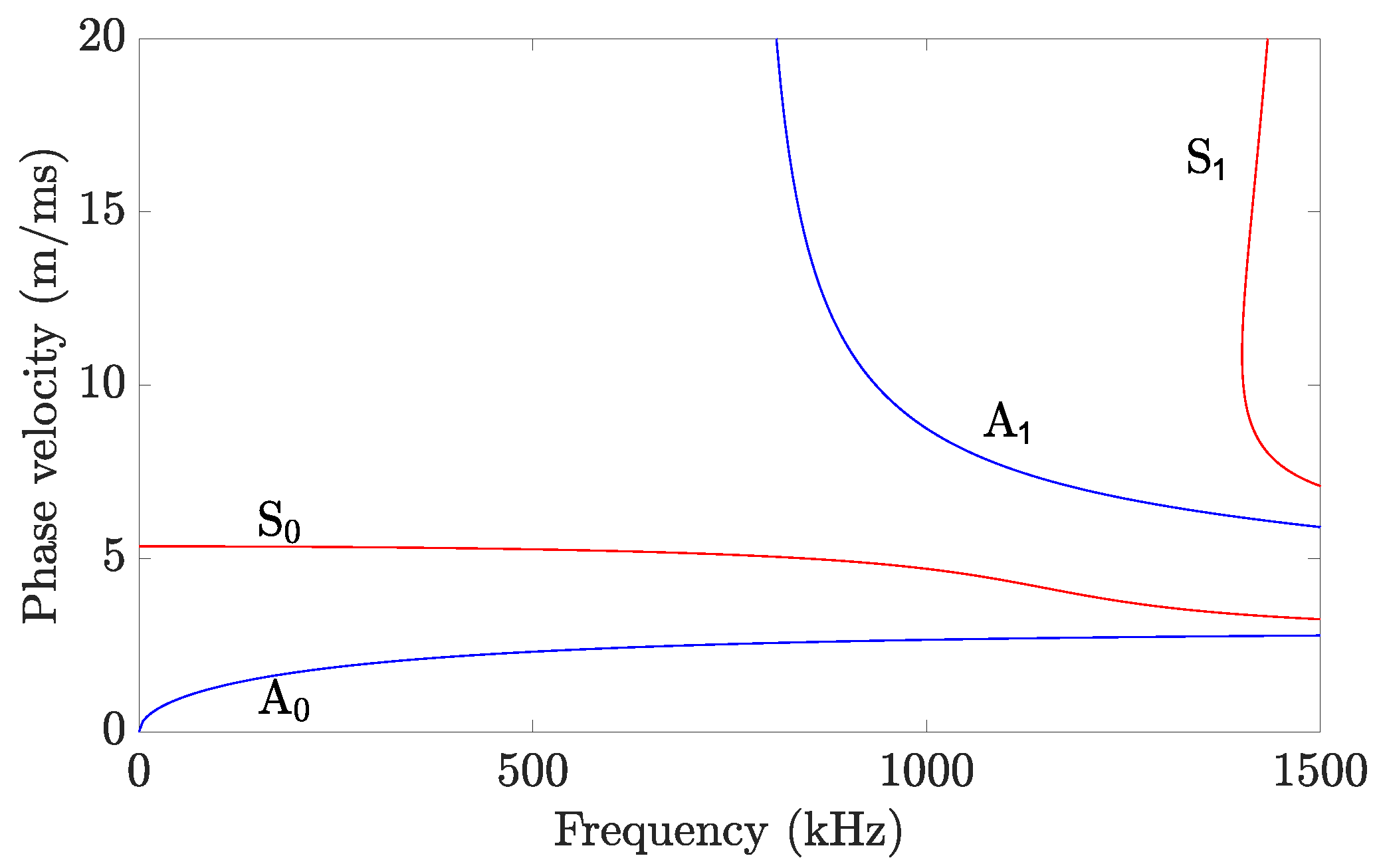
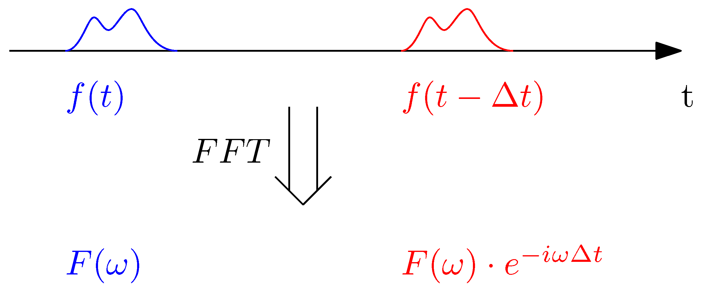
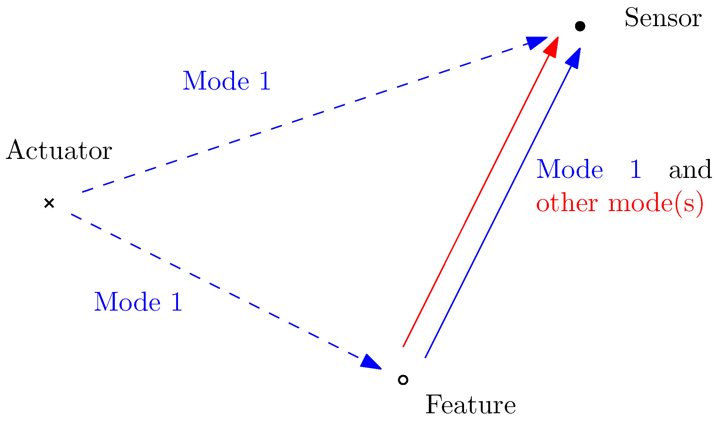
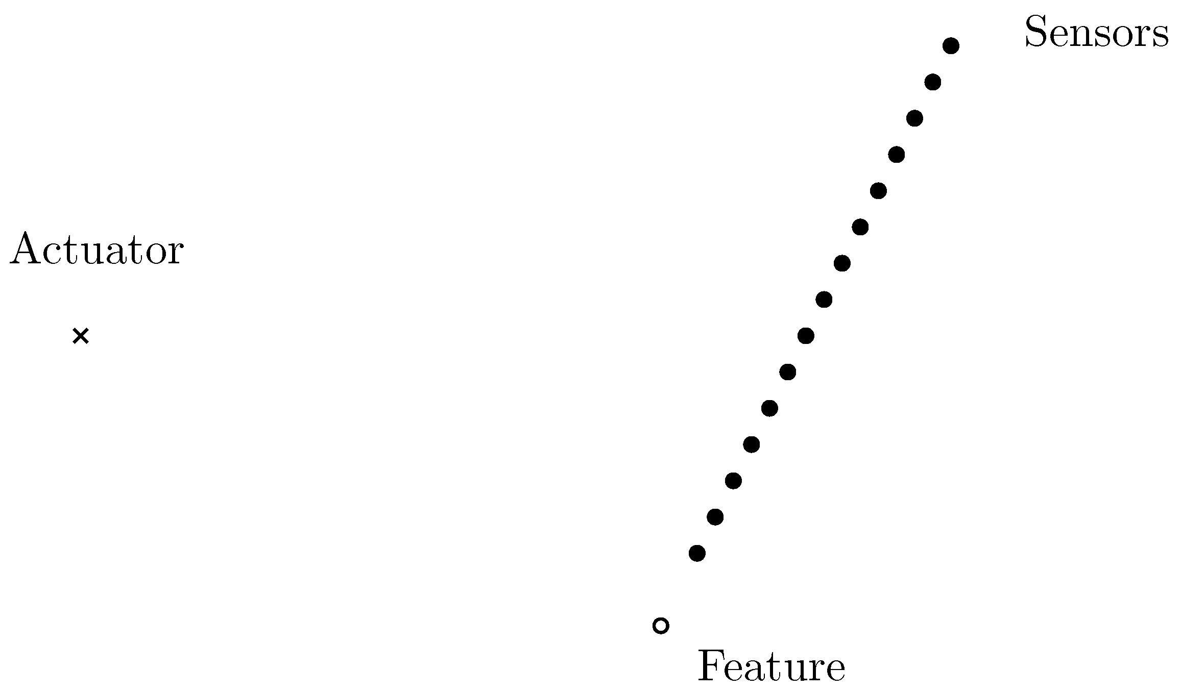
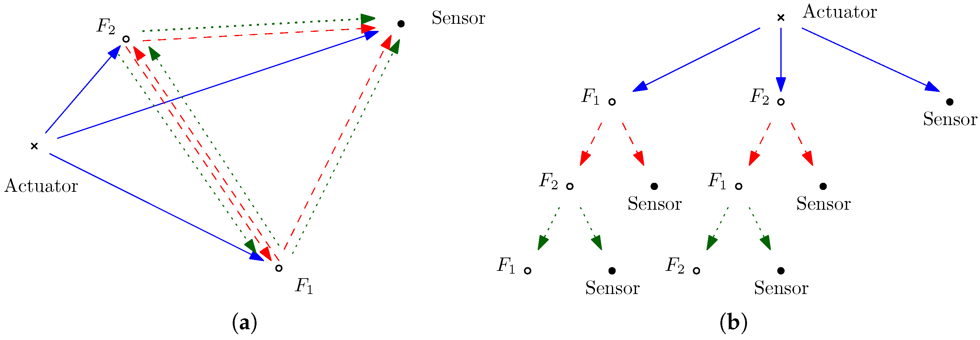
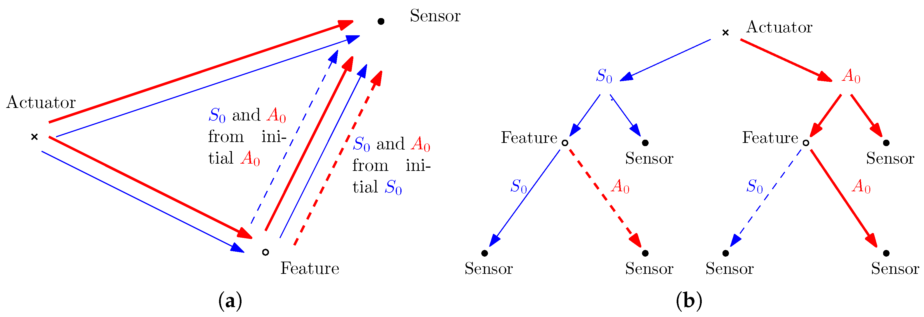
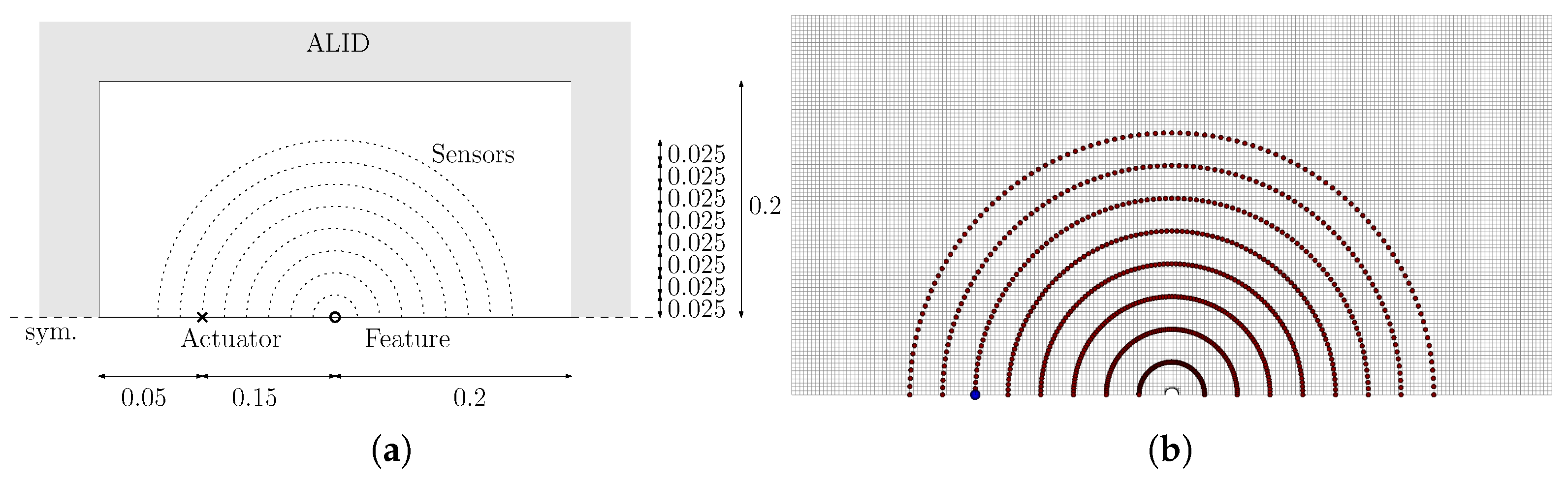
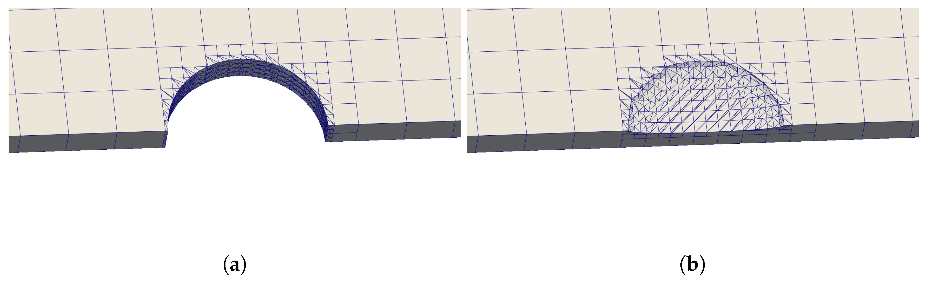
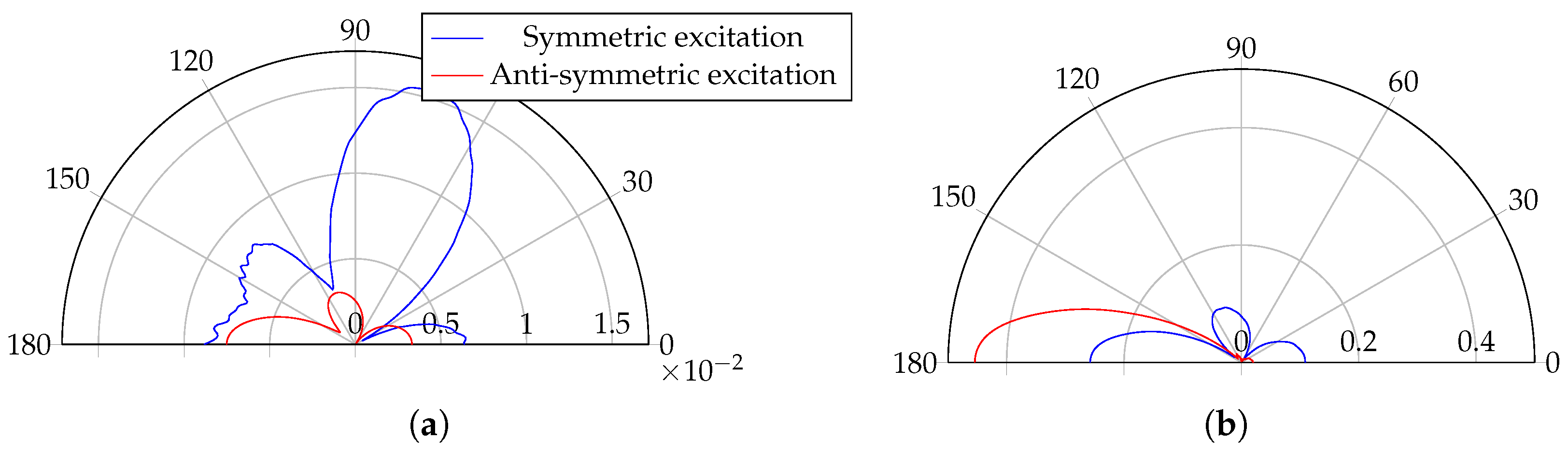
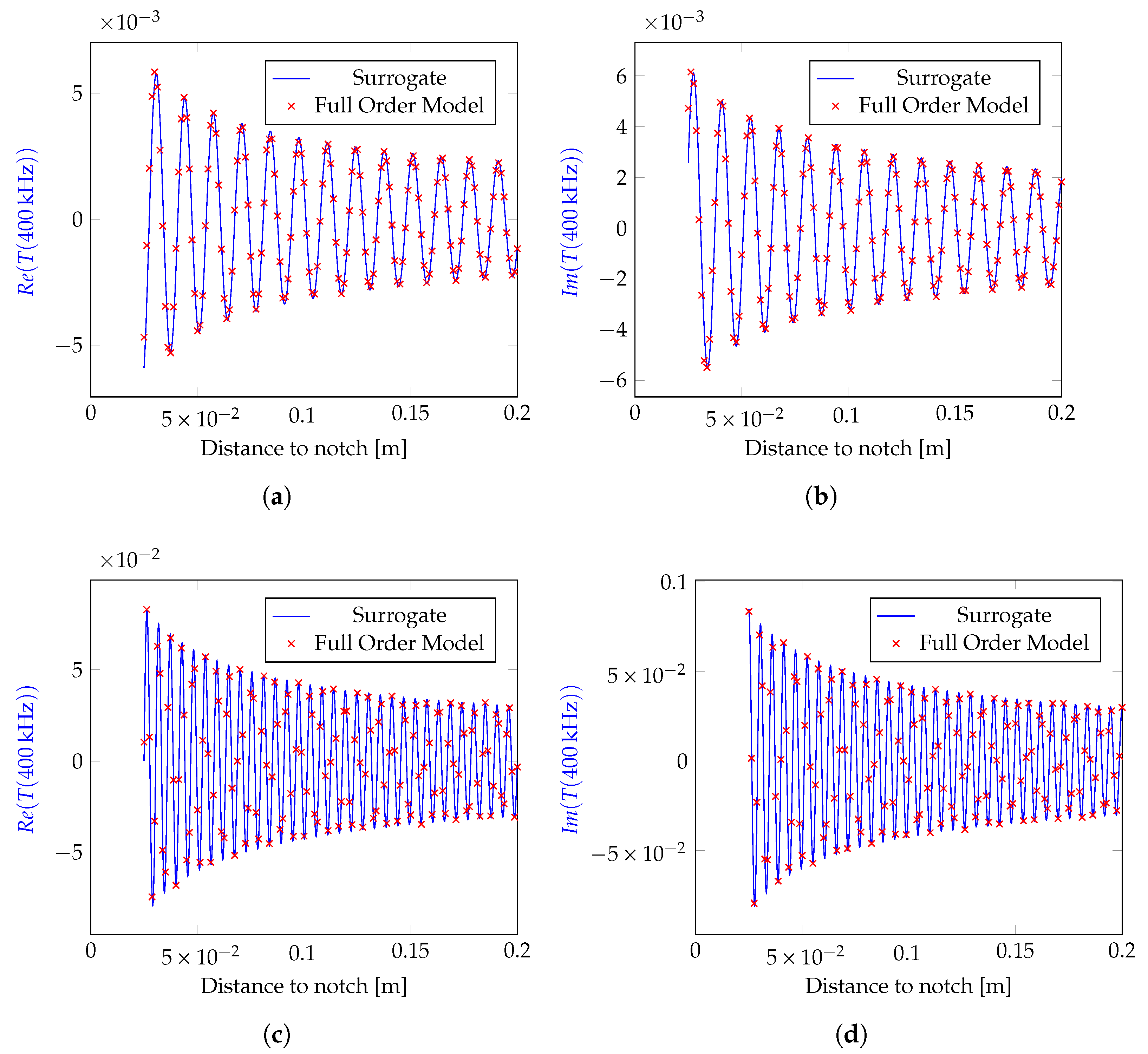
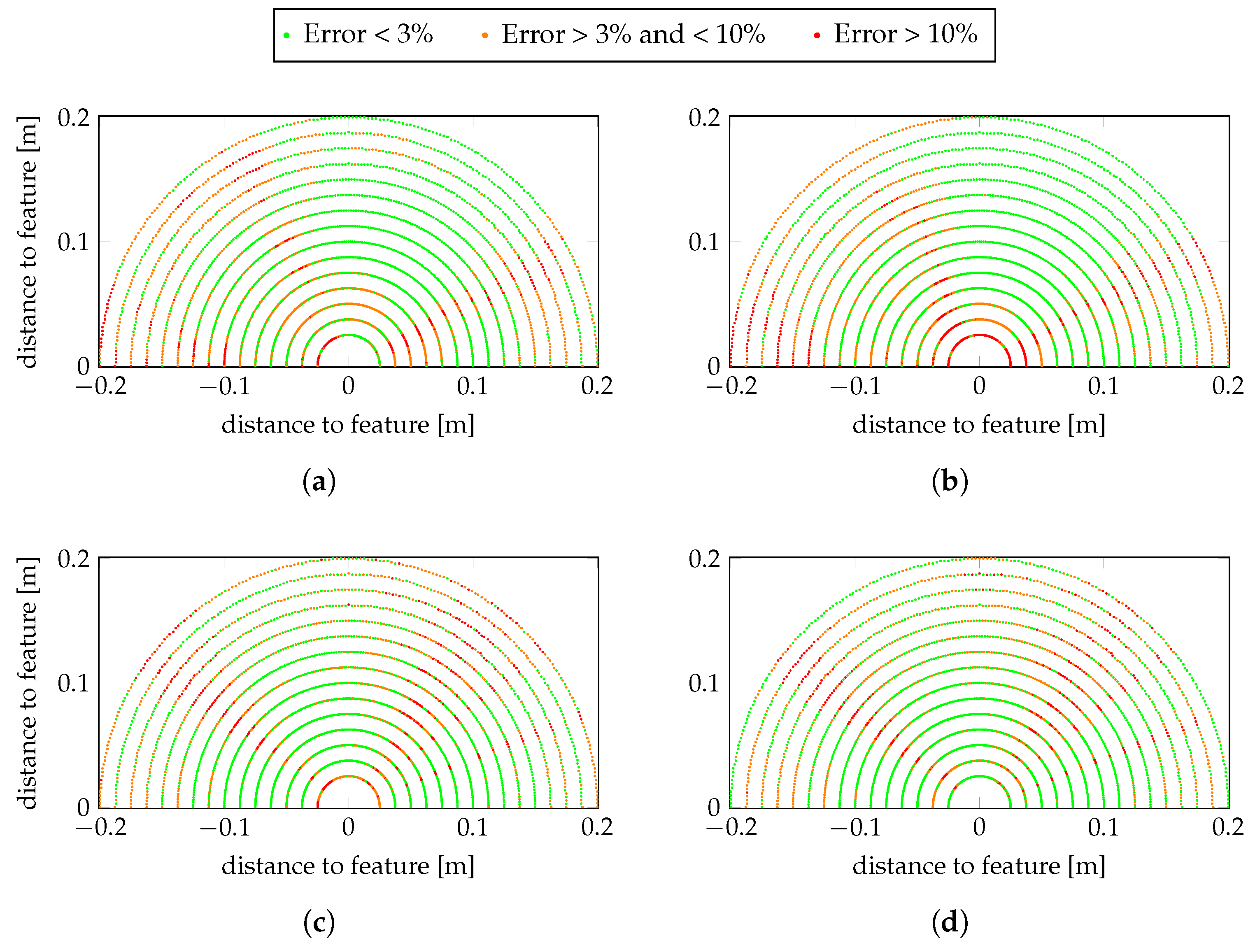
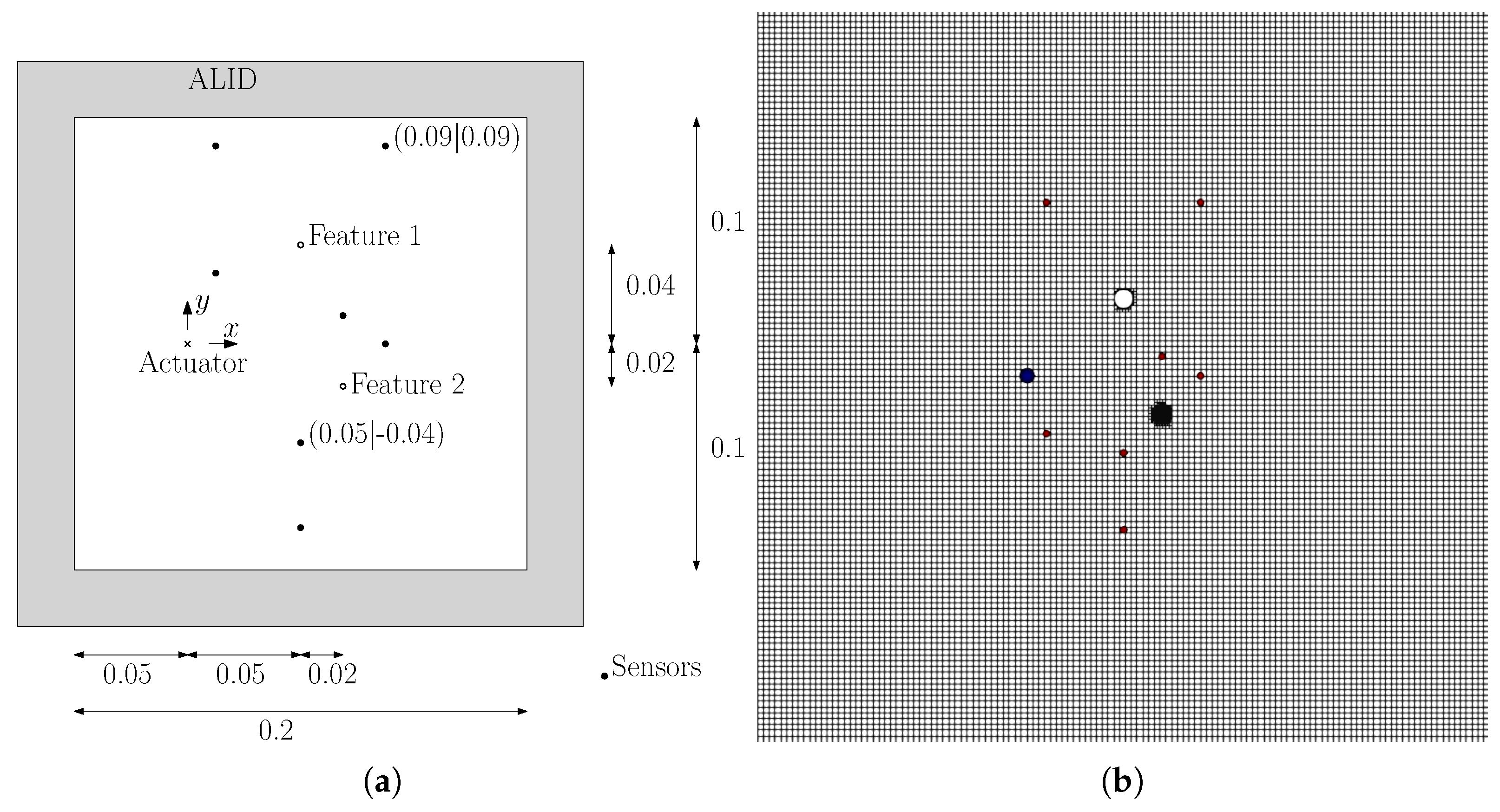
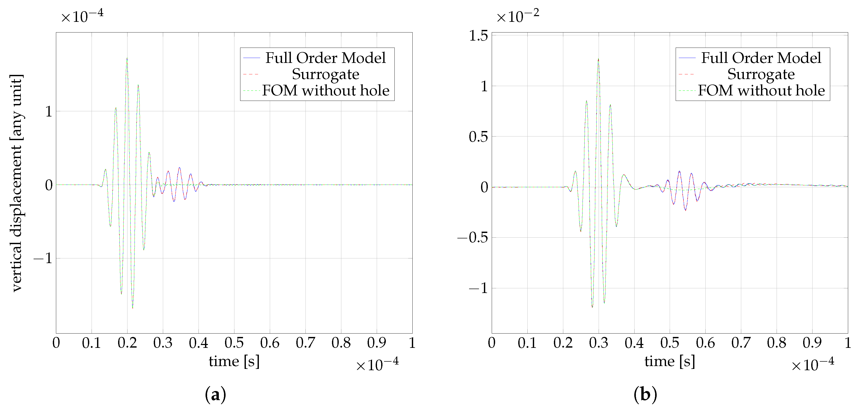
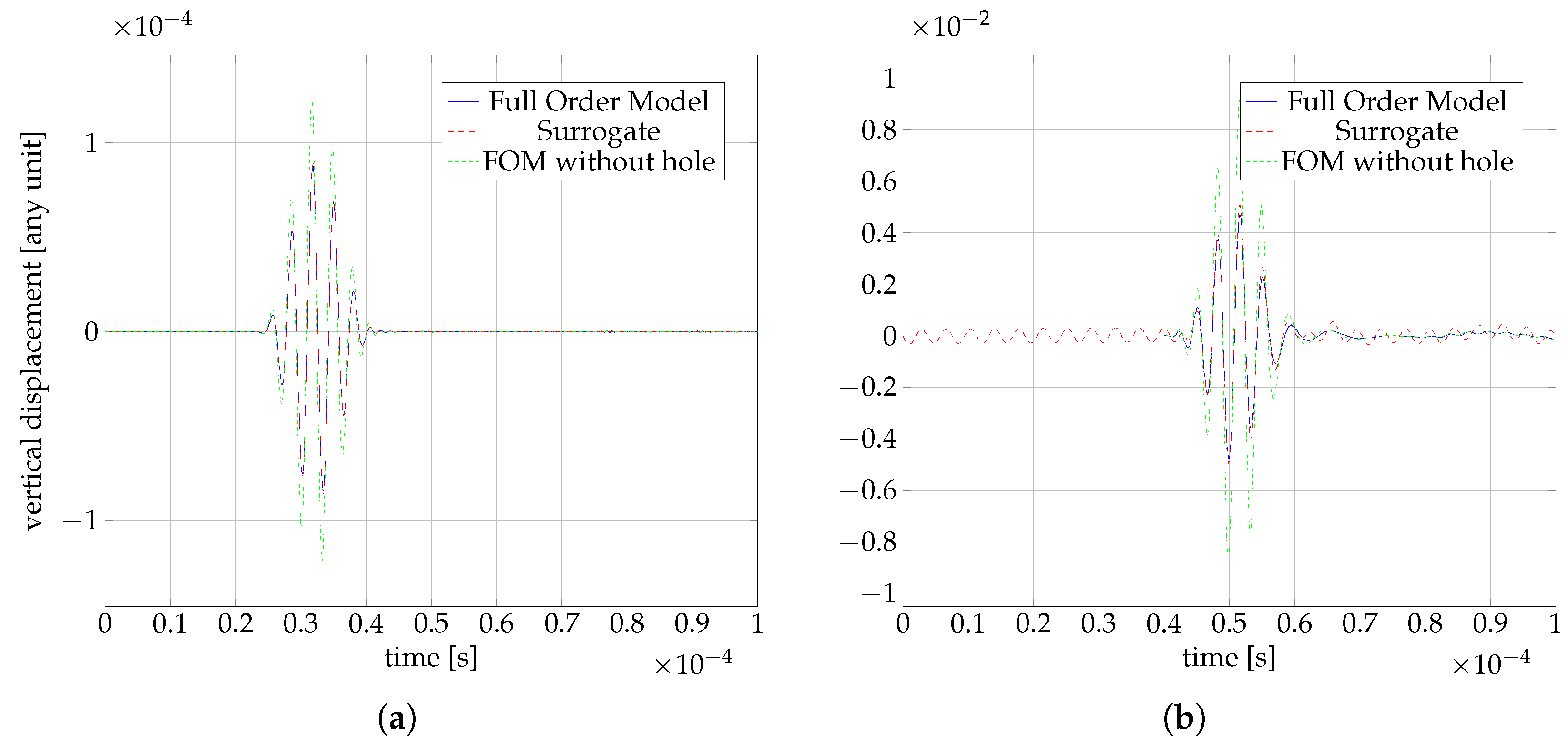
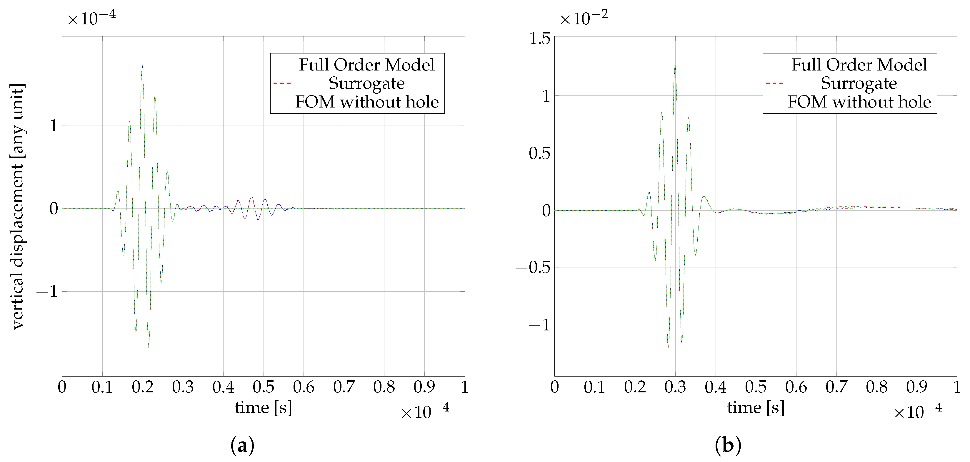
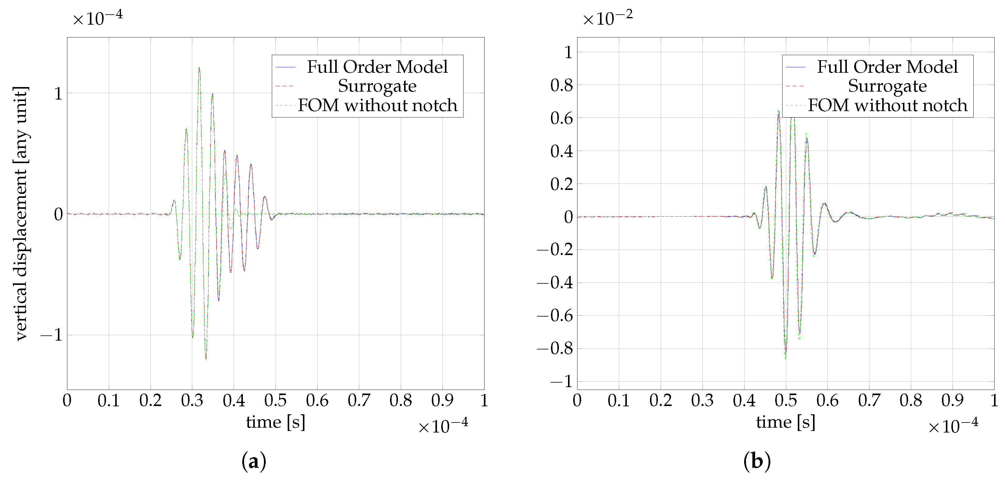
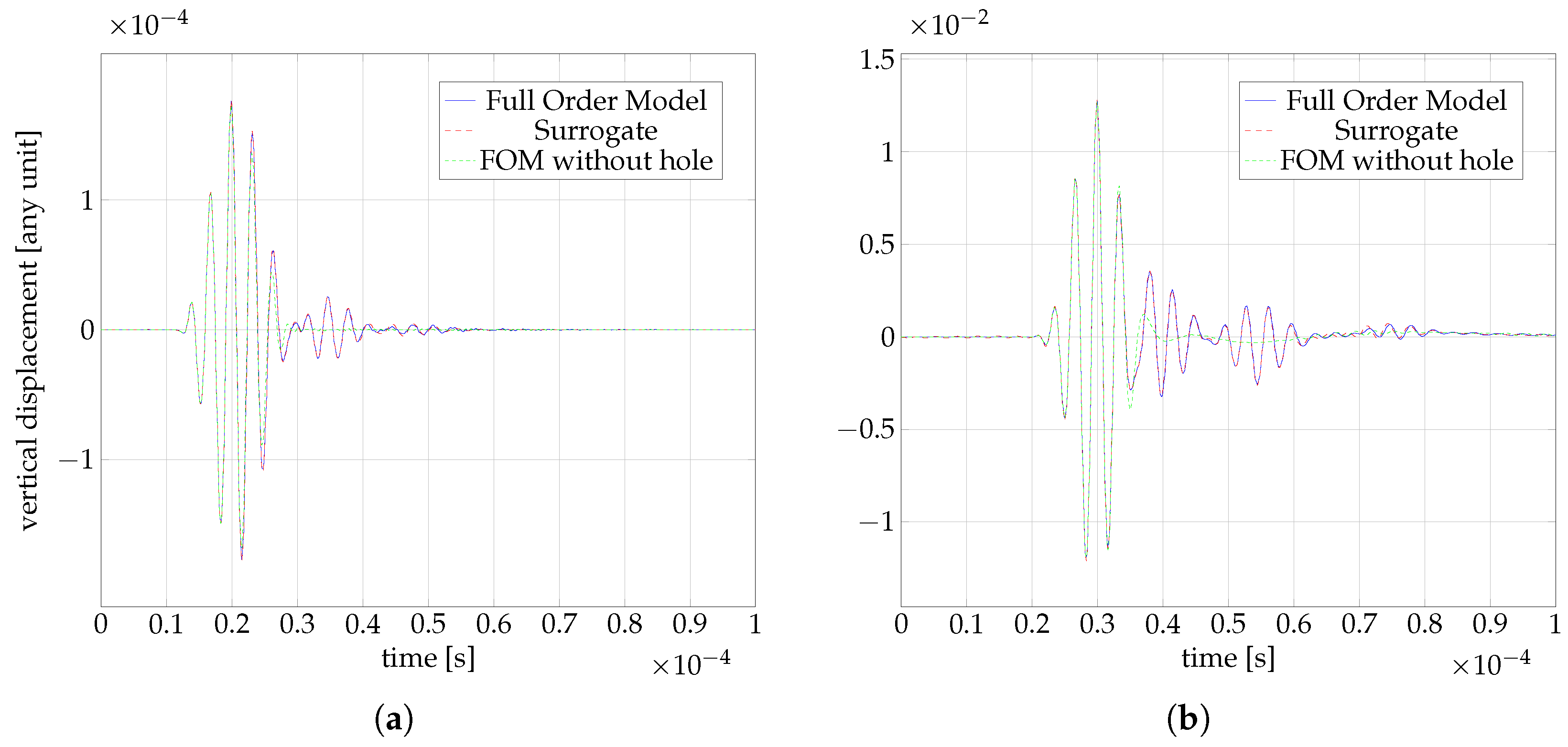
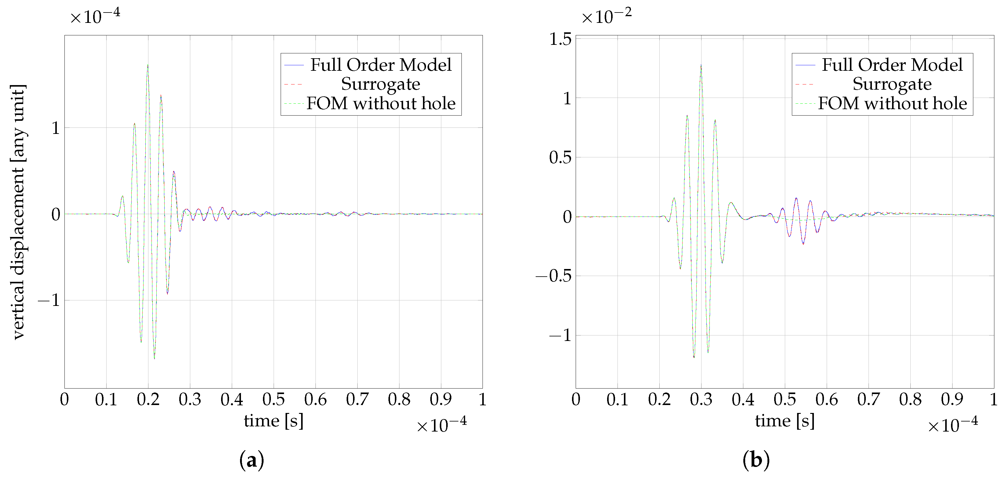
Disclaimer/Publisher’s Note: The statements, opinions and data contained in all publications are solely those of the individual author(s) and contributor(s) and not of MDPI and/or the editor(s). MDPI and/or the editor(s) disclaim responsibility for any injury to people or property resulting from any ideas, methods, instructions or products referred to in the content. |
© 2025 by the authors. Licensee MDPI, Basel, Switzerland. This article is an open access article distributed under the terms and conditions of the Creative Commons Attribution (CC BY) license (https://creativecommons.org/licenses/by/4.0/).