
Time-Series Prediction of Failures in an Industrial Assembly Line Using Artificial Learning


Abstract
Featured Application
Abstract

1. Introduction
2. Significance and Novelty of the Study
- The configuration data are collected in the aerospace industry. Unlike many other sectors, the safety factor in structural design typically does not exceed 1.2, generally, with some designs even falling below 1.0. This is primarily due to the stringent requirement for lightweight structures. Nonetheless, structural integrity must not be compromised. The assembly phase—being the final stage of production—demands precise component compatibility. Any failure occurring during assembly can halt the entire production line and potentially result in catastrophic in-service damage to the aircraft or spacecraft. Such failures are associated with severe economic consequences.
- The aerospace sector is distinguished by its low-volume, high-precision production and assembly requirements. These unique characteristics necessitate domain-specific attention and pose particular challenges not encountered in other industries.
- Structural damage in aerospace systems may result from various factors, including fatigue, corrosion, manufacturing defects (e.g., voids, inclusions, dislocations), processing flaws (e.g., surface scratches, weld discontinuities, chevron notches, microstructural alterations), mechanical loading (tension/compression, bending, torsion, shear, pressure), impact, wear, creep, friction, hydrogen embrittlement, high temperature, and vibration. While damage tolerance design can mitigate many of these effects, human-induced errors remain difficult to eliminate. Regardless of the underlying cause, early fault prediction can help to prevent such failures.
- Not all AL techniques are suitable for time-series data. Some methods are good at image processing, while others are more effective in modelling. Time-series data demand specific attention due to their unimodal nature and the necessity to incorporate time lags as both input and output for accurate prediction. Furthermore, convergence during the training phase of learning algorithms is not always guaranteed.
- This study not only compares prediction performance but also evaluates different methods with distinct underlying architectures. At the end, the most suitable technique for modelling aerospace assembly-related time series is identified.
- The novelty of this research lies in both its use of domain-specific aerospace assembly data and the implementation of diverse and specialised modelling techniques. Modelling and prediction continue to be an active area of inquiry for both researchers and industry practitioners.
3. Materials and Methods
3.1. Data Collecting
3.2. Preliminary Studies on the Data
3.3. Statistical Tools for Evaluating the Model Performances
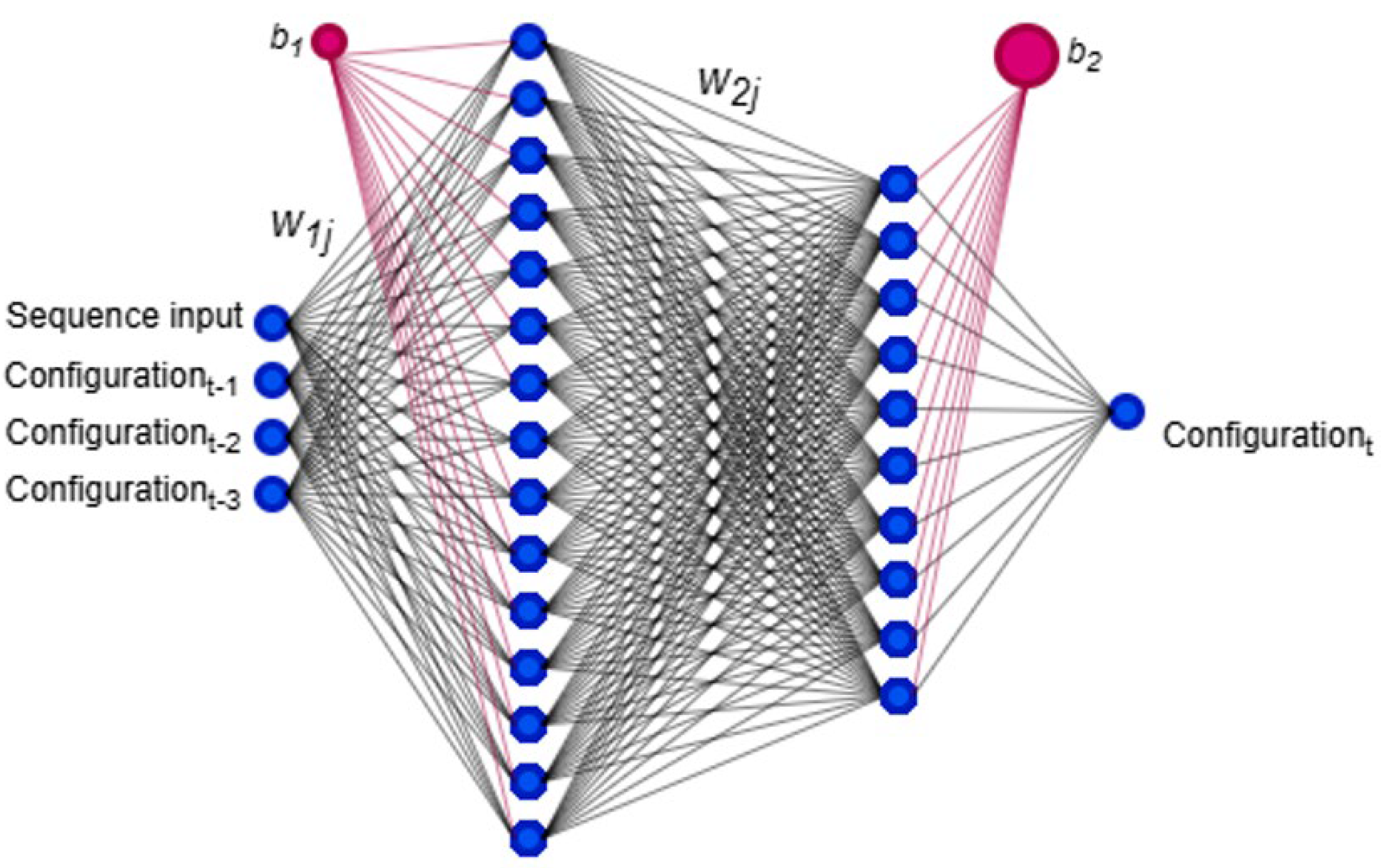
3.4. Modelling Using the NAR Network
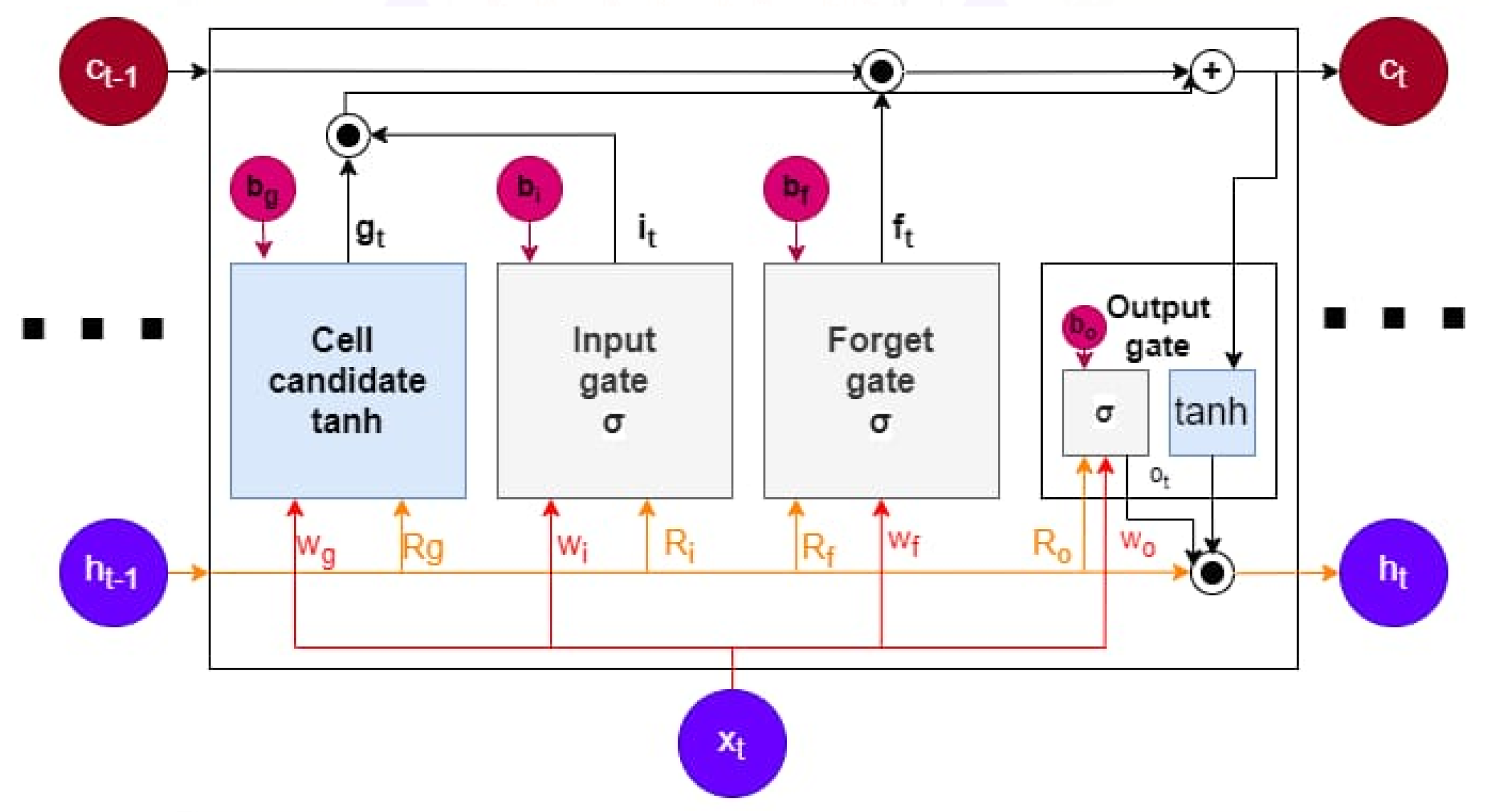
3.5. Modelling Using the LSTM Network
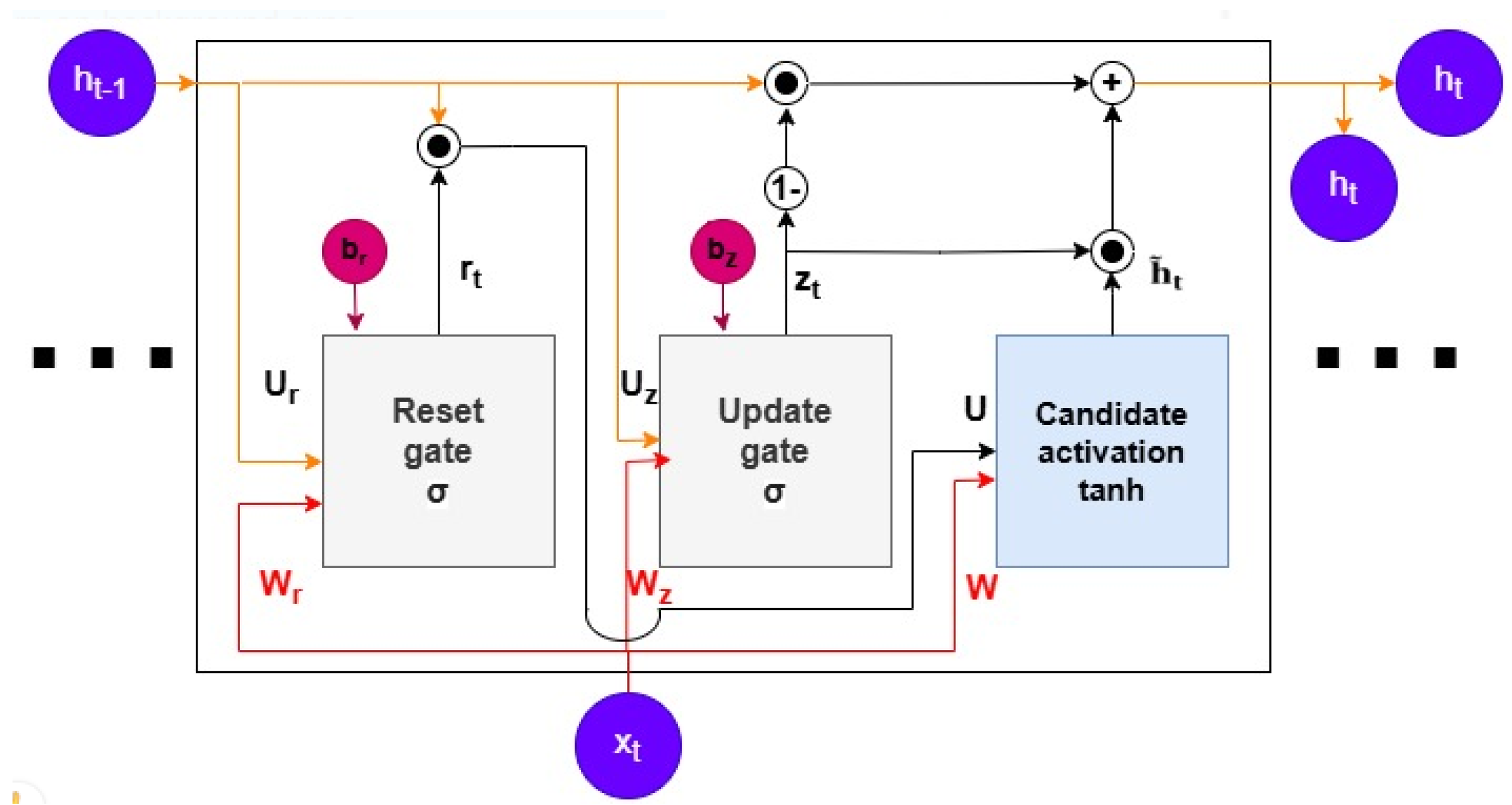
3.6. Modelling Using the GRU Network
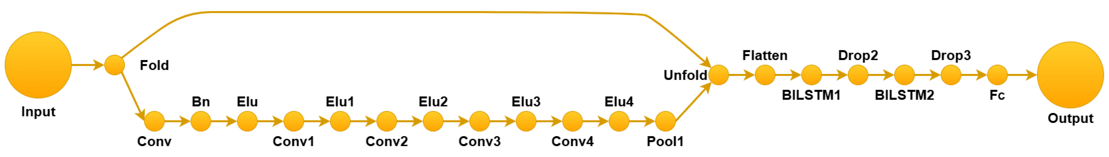
3.7. Modelling Using the CNN-RNN Hybrid Network
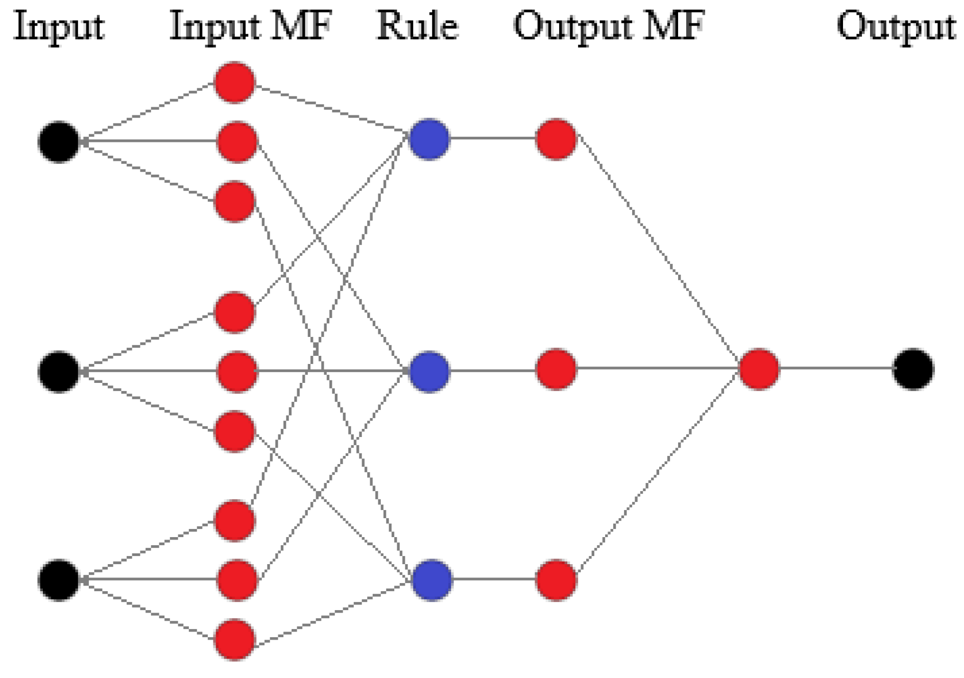
3.8. Modelling Using ANFIS
3.9. Modelling Using MLP
4. Results and Discussion
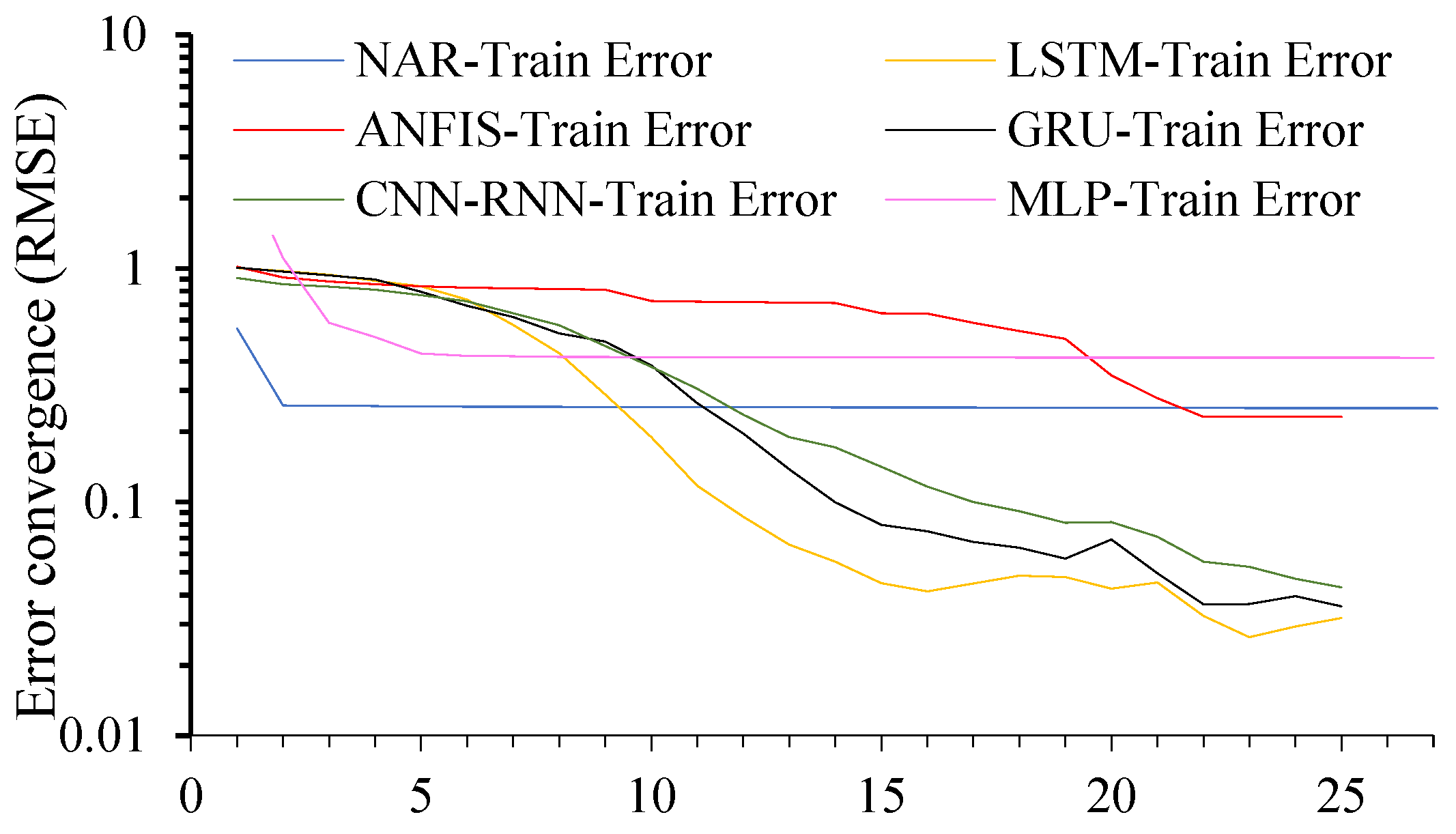
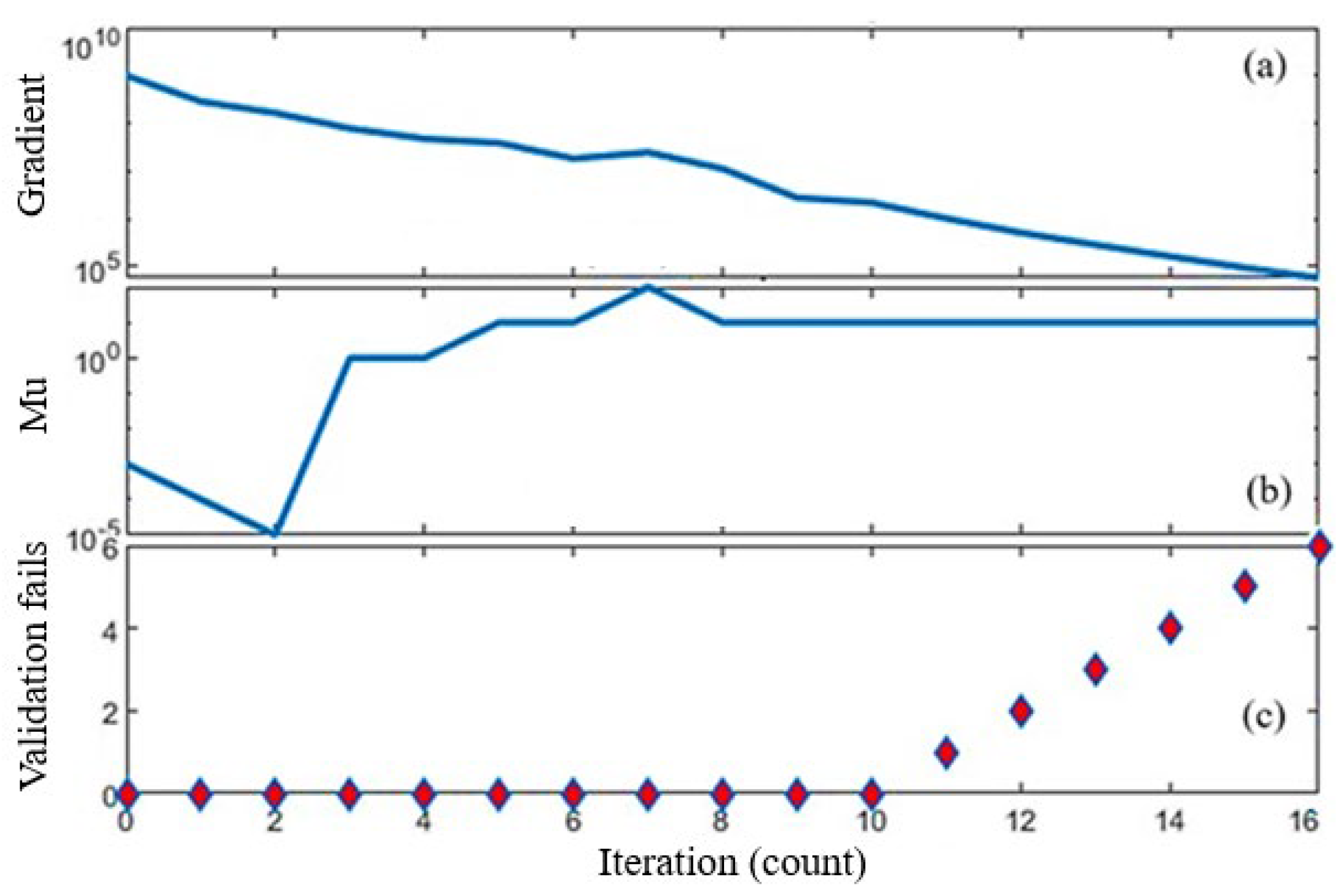
4.1. Error Convergences and Performance Metrics
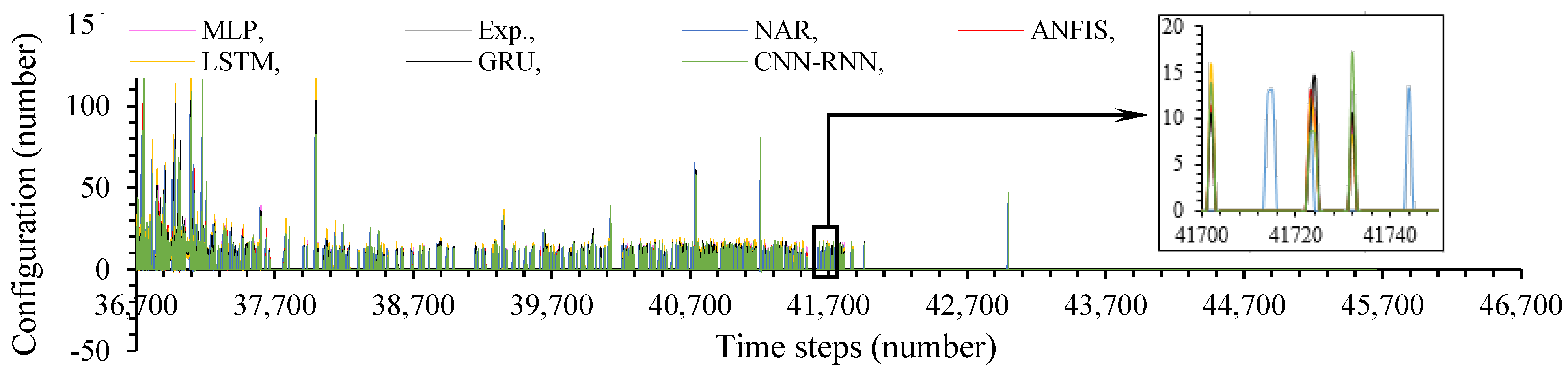
4.2. Predicted Data
4.3. Residual Analysis
4.4. Variance Analysis
4.5. Discussion
5. Conclusions
Author Contributions
Funding
Data Availability Statement
Acknowledgments
Conflicts of Interest
Abbreviations
| Abbreviation | Full Form |
| ACF | Autocorrelation Function |
| ADAM | Adaptive Moment Estimation |
| AL | Artificial learning |
| ANFIS | Adaptive neuro-fuzzy inference system |
| AR | Autoregressive |
| BILSTM | Bidirectional long short-term memory |
| CNN-RNN | Convolutional neural network–recurrent neural network hybrid |
| CPU | Central Processing Unit |
| ELU | Exponential Linear Unit |
| FCM | Fuzzy C-means |
| FIS | Fuzzy inference system |
| FNN | Fuzzy neural network |
| GRU | Gated recurrent unit |
| LSTM | Long short-term memory |
| MAE | Mean absolute error |
| MBE | Mean bias error |
| MF | Membership function |
| ML | Machine learning |
| MLP | Multilayer perceptron |
| MSE | Mean squared error |
| MAPE | Mean absolute percentage error |
| NAR | Nonlinear autoregressive |
| NARX | Nonlinear autoregressive with exogenous inputs |
| PACF | Partial Autocorrelation Function |
| RNN | Recurrent neural network |
| RMSE | Root mean square error |
| RMSProp | Root mean square propagation |
| R | Correlation coefficient |
| R2 | Coefficient of determination |
| SGD | Stochastic gradient descent |
| SVR | Support Vector Regression |
References
- Montgomery, D.C. Introduction to Statistical Quality Control, 8th ed.; John Wiley & Sons, Inc.: Hoboken, NJ, USA, 2019; p. 768. [Google Scholar]
- Kusiak, A. Smart manufacturing. Int. J. Prod. Res. 2018, 56, 508–517. [Google Scholar] [CrossRef]
- Tobon-Mejia, D.A.; Medjaher, K.; Zerhouni, N.; Tripot, G. A Data-Driven Failure Prognostics Method Based on Mixture of Gaussians Hidden Markov Models. IEEE Trans. Reliab. 2012, 61, 491–503. [Google Scholar] [CrossRef]
- Amiroh, K.; Rahmawati, D.; Wicaksono, A.Y. Intelligent System for Fall Prediction Based on Accelerometer and Gyroscope of Fatal Injury in Geriatric. Jurnal Nasional Teknik Elektro 2021, 10, 154–159. [Google Scholar] [CrossRef]
- Çelen, S. Availability and modelling of microwave belt dryer in food drying. J. Tekirdag Agric. Fac. 2016, 13, 71–83. [Google Scholar]
- Karacabey, E.; Aktaş, T.; Taşeri, L.; Uysal Seçkin, G. Examination of different drying methods in Sultana Seedless Grapes in terms of drying kinetics, energy consumption and product quality. J. Tekirdag Agric. Fac. 2020, 17, 53–65. [Google Scholar] [CrossRef]
- Hopfield, J.J. Neural networks and physical systems with emergent collective computational abilities. Proc. Natl. Acad. Sci. USA 1982, 79, 2554–2558. [Google Scholar] [CrossRef]
- Werbos, P.J. Generalization of backpropagation with application to a recurrent gas market model. Neural Netw. 1988, 1, 339–356. [Google Scholar] [CrossRef]
- Hochreiter, S.; Schmidhuber, J. Long Short-Term Memory. Neural Comput. 1997, 9, 1735–1780. [Google Scholar] [CrossRef]
- Cho, K.; van Merriënboer, B.; Gulcehre, C.; Bahdanau, D.; Bougares, F.; Schwenk, H.; Bengio, Y. Learning phrase representations using RNN encoder–decoder for statistical machine translation. In Proceedings of the 2014 Conference on Empirical Methods in Natural Language Processing (EMNLP), Doha, Qatar, 25–29 October 2014; pp. 1724–1734. [Google Scholar]
- Hu, Y.; Wong, Y.; Wei, W.; Du, Y.; Kankanhalli, M.; Geng, W. A novel attention-based hybrid CNN-RNN architecture for sEMG-based gesture recognition. PLoS ONE 2018, 13, e0206049. [Google Scholar] [CrossRef]
- Shekar, P.R.; Mathew, A.; Sharma, K.V. A hybrid CNN–RNN model for rainfall–runoff modeling in the Potteruvagu watershed of India. CLEAN—Soil Air Water 2024, 53, 2300341. [Google Scholar] [CrossRef]
- Liu, H.; Jin, Y.; Song, X.; Pei, Z. Rate of Penetration Prediction Method for Ultra-Deep Wells Based on LSTM–FNN. Appl. Sci. 2022, 12, 7731. [Google Scholar] [CrossRef]
- Chumakova, E.V.; Korneev, D.G.; Chernova, T.A.; Gasparian, M.S.; Ponomarev, A.A. Comparison of the application of FNN and LSTM based on the use of modules of artificial neural networks in generating an individual knowledge testing trajectory. J. Eur. Des Systèmes Automatisés 2023, 56, 213–220. [Google Scholar] [CrossRef]
- Yu, H.-C.; Wang, Q.-A.; Li, S.-J. Fuzzy Logic Control with Long Short-Term Memory Neural Network for Hydrogen Production Thermal Control System. Appl. Sci. 2024, 14, 8899. [Google Scholar] [CrossRef]
- Liu, F.; Dong, T.; Liu, Q.; Liu, Y.; Li, S. Combining fuzzy clustering and improved long short-term memory neural networks for short-term load forecasting. Electr. Pow. Syst. Res. 2024, 226, 109967. [Google Scholar] [CrossRef]
- Wang, W.; Shao, J.; Jumahong, H. Fuzzy inference-based LSTM for long-term time series prediction. Sci. Rep. 2023, 13, 20359. [Google Scholar] [CrossRef]
- Xin, T.L.L. Fuzzy Embedded Long Short-Term Memory (FE-LSTM) with Applications in Stock Trading; Final Year Project (FYP); Nanyang Technological University: Singapore, 2022. [Google Scholar]
- Liu, L.; Fei, J.; An, C. Adaptive Sliding Mode Long Short-Term Memory Fuzzy Neural Control for Harmonic Suppression. IEEE Access 2021, 9, 69724–69734. [Google Scholar] [CrossRef]
- Suppiah, R.; Kim, N.; Sharma, A.; Abidi, K. Fuzzy inference system (FIS)—Long short-term memory (LSTM) network for electromyography (EMG) signal analysis. Biomed. Phys. Eng. Express 2022, 8, 065032. [Google Scholar] [CrossRef]
- Topaloğlu Yıldız, Ş.; Yıldız, G.; Cin, E. Mathematical programming and simulation modeling based solution approach to worker assignment and assembly line balancing problem in an electronics company. Afyon Kocatepe Univ. J. Econ. Adm. Sci. 2020, 22, 57–73. [Google Scholar] [CrossRef]
- Demirkol Akyol, Ş. Linear programming approach for type-2 assembly line balancing and workforce assignment problem: A case study. Dokuz Eylül Univ. Fac. Eng. J. Sci. Eng. 2023, 25, 121–129. (In Turkish) [Google Scholar] [CrossRef]
- Korkmaz, C.; Kacar, İ. Explaining Data Preprocessing Methods for Modeling and Forecasting with the Example of Product Drying. J. Tekirdag Agric. Fac. 2024, 21, 482–500. (In Turkish) [Google Scholar] [CrossRef]
- Kutner, M.H.; Nachtsheim, C.J.; Neter, J. Applied Linear Regression Models; McGraw-Hill Higher Education: New York, NY, USA, 2003. [Google Scholar]
- Seber, G.A.F.; Lee, A.J. Linear Regression Analysis; Wiley: Hoboken, NJ, USA, 2012. [Google Scholar]
- Gujarati, D.N.; Porter, D.C. Basic Econometrics, 5th ed.; McGraw-Hill/Irwin: New York, NY, USA, 2009; p. 921. [Google Scholar]
- Montesinos López, O.A.; Montesinos López, A.; Crossa, J. Fundamentals of Artificial Neural Networks and Deep Learning. In Multivariate Statistical Machine Learning Methods for Genomic Prediction; Montesinos López, O.A., Montesinos López, A., Crossa, J., Eds.; Springer International Publishing: Cham, Switzerland, 2022; pp. 379–425. [Google Scholar]
- He, K.; Zhang, X.; Ren, S.; Sun, J. Delving deep into rectifiers: Surpassing human-level performance on imagenet classification. In Proceedings of the 2015 IEEE International Conference on Computer Vision (ICCV), Santiago, Chile, 7–13 December 2015; pp. 1026–1034. [Google Scholar]
- Chung, J.; Gulcehre, C.; Cho, K.; Bengio, Y. Empirical Evaluation of Gated Recurrent Neural Networks on Sequence Modeling. In Proceedings of the NIPS 2014 Workshop on Deep Learning, Montreal, QC, Canada, 8–13 December 2014. [Google Scholar]
- Graves, A.; Fernández, S.; Schmidhuber, J. Bidirectional LSTM Networks for Improved Phoneme Classification and Recognition; Springer: Berlin/Heidelberg, Germany, 2005; pp. 799–804. [Google Scholar]
- Yenter, A.; Verma, A. Deep CNN-LSTM with combined kernels from multiple branches for IMDb review sentiment analysis. In Proceedings of the 2017 IEEE 8th Annual Ubiquitous Computing, Electronics and Mobile Communication Conference (UEMCON), New York, NY, USA, 19–21 October 2017; pp. 540–546. [Google Scholar]
- Kacar, İ.; Korkmaz, C. Prediction of agricultural drying using multi-layer perceptron network, long short-term memory network and regression methods. Gümüşhane Univ. J. Sci. Technol. 2022, 12, 1188–1206. (In Turkish) [Google Scholar] [CrossRef]
- Hussain, S.; AlAlili, A. A hybrid solar radiation modeling approach using wavelet multiresolution analysis and artificial neural networks. Appl. Energ. 2017, 208, 540–550. [Google Scholar] [CrossRef]
- Aslanargun, A.; Mammadov, M.; Yazici, B.; Asma, S. Comparison of ARIMA, neural networks and hybrid models in time series: Tourist arrival forecasting. J. Stat. Comput. Simul. 2007, 77, 29–53. [Google Scholar] [CrossRef]
- Duan, W.; Zhang, K.; Wang, W.; Dong, S.; Pan, R.; Qin, C.; Chen, H. Parameter prediction of lead-bismuth fast reactor under various accidents with recurrent neural network. Appl. Energ. 2025, 378, 124790. [Google Scholar] [CrossRef]
- Zhu, R.; Sun, Q.; Han, X.; Wang, H.; Shi, M. A novel dual-channel deep neural network for tunnel boring machine slurry circulation system data prediction. Adv. Eng. Softw. 2025, 201, 103853. [Google Scholar] [CrossRef]
- Yu, Z.; He, X.; Montillet, J.-P.; Wang, S.; Hu, S.; Sun, X.; Huang, J.; Ma, X. An improved ICEEMDAN-MPA-GRU model for GNSS height time series prediction with weighted quality evaluation index. GPS Solut. 2025, 29, 113. [Google Scholar] [CrossRef]
- Khan, F.M.; Gupta, R. ARIMA and NAR based prediction model for time series analysis of COVID-19 cases in India. J. Saf. Sci. Resil. 2020, 1, 12–18. [Google Scholar] [CrossRef]
- Olmedo, M.T.C.; Mas, J.F.; Paegelow, M. The Simulation Stage in LUCC Modeling; Olmedo, M.T.C., Paegelow, M., Mas, J.F., Escobar, F., Eds.; Springer International Publishing: Cham, Switzerland, 2018; pp. 451–455. [Google Scholar]
- Pinkus, A. Approximation theory of the MLP model in neural networks. Acta Numer. 1999, 8, 143–195. [Google Scholar] [CrossRef]
- Korkmaz, C.; Kacar, İ. Time-series prediction of organomineral fertilizer moisture using machine learning. Appl. Soft Comput. 2024, 165, 112086. [Google Scholar] [CrossRef]


| Parameter | Value |
|---|---|
| Stopping criteria of training | MSE = 0.0 or 6 consecutive validation fails or max 1000 epochs or min 1 × 10⁻⁷ gradient or min 1 × 10¹⁰ mu |
| Number of hidden layers | 2 |
| Number of neurons in each hidden layer | 15 and 10, respectively |
| Activation functions | Hyperbolic tangent sigmoid in hidden layers, linear in the output layer. |
| Training algorithm | Levenberg–Marquardt |
| Delay (d) | 3, feedback of Configurationt−1, Configurationt−2, Configurationt−3 |
| Inputs | Configurationt−1, Configurationt−2, Configurationt−3 |
| Output | Configurationt |
| Output threshold | 0.99 |
| Learning rate | 0.1 |
| Momentum | 0.1 |
| Learning threshold | 0.0001 |
| Batch size | 80% (modelling *), 20% (forecasting); all data normalised |
| Layer | Configuration | Parameters |
|---|---|---|
| Sequential input layer | Time-series data | Configuration |
| Input variable(s) | 3 lag(s) of output | Configurationt−1, Configurationt−2, Configurationt−3 |
| LSTM layer(s) | 1 layer | Stack size: 80% (modelling), 20% (forecasting); all data normalised |
| Hidden unit (count) | 64 | Gates: sigmoid, State: tanh |
| Dropout layer | After LSTM layer | Dropout probability: 0.2 |
| Fully connected layer | 1 unit | Number of responses = 1 (the configuration data) |
| Output | 1 unit | Regression layer: Loss function = MSE |
| Training algorithm (Solver) | ADAM | Initial learning rate: 0.03 Learning rate: piecewise (drop factor: 0.5, drop period: 100 epochs) Gradient explosion threshold: 0.8 L2 regularisation: 0.01 Shuffle: every epoch |
| Weight initialisations | He initialiser [28] | |
| Epochs | Iterations per epoch = 1 | 100 |
| CNN Design | |
|---|---|
| Layers Configuration | Parameters |
| Sequence input layer | Feedback of three delays of the output [3 1 1] |
| Sequence folding layer | Sequence input layer → 2D format |
| Convolution2d layer | Dilation factor = [1 1] |
| Batch normalisation layer | where is mean |
| ELU layer | |
| Convolution2d layer | Dilation factor = [2 2] |
| ELU layer | |
| Convolution2d layer | Dilation factor = [4 4] |
| ELU layer | |
| Convolution2d layer | Dilation factor = [8 8] |
| ELU layer | |
| Convollution2d layer | Dilation factor = [16 16] |
| ELU layer | |
| Average pooling2d layer | Pool size = 1, stride = [5 5] |
| Sequence unfolding layer | -- |
| Flatten layer | It converts H-by-W-by-C-by-N-by-S to (H*W*C)-by-N-by-S |
| RNN design | |
| BILSTM layer | Hidden unit = 64 |
| Dropout layer | Probability = 0.2 |
| BILSTM layer | Hidden unit = 16 Output the last time step of the sequence |
| Fully connected layer | Number of responses = 1 (configuration failure) |
| Regression layer | Loss function = |
| Layer | Configuration | Parameters |
|---|---|---|
| Output variable | Time-series data | Configuration |
| Input variable(s) | 3 lag(s) of output | Configurationt−1, Configurationt−2, Configurationt−3 |
| Batch size | -- | 80% (modelling), 20% (forecasting); normalised |
| Fuzzification and data clustering | FCM | Input MF: Gauss; clusters: 10 for each input Partition matrix exponent, Initial step size: 0.01; step size decrement rate: 0.9; step size increase rate: 1.1 |
| Defuzzification | Output MF | Zero-order Sugeno and first-order Sugeno |
| Decision-making | AND | -- |
| Optimisation method | Hybrid | -- |
| Epochs | Iterations per epoch = 1 | 10, 50, and 100 epochs |
| Metrics | NAR | LSTM | ANFIS | GRU | CNN-RNN | MLP |
|---|---|---|---|---|---|---|
| Total data count | 45,654 | 45,654 | 45,654 | 45,654 | 45,654 | 45,654 |
| Training data count | 9130 | 9130 | 9130 | 9130 | 9130 | 9130 |
| MAE (unit) * | 2.592 | 5.081 | 2.805 | 4.124 | 5.063 | 2.122 |
| MAPE (%) | 0.895 | 5.081 | 0.862 | 2.848 | 2.948 | 0.876 |
| ME (unit) | 1.279 | 3.061 | 1.296 | 2.488 | 3.632 | 1.145 |
| MSE (unit2) | 1.225 | 17.297 | 1.985 | 8.243 | 30.814 | 2.011 |
| RMSE (unit) | 1.107 | 4.159 | 1.409 | 2.871 | 5.551 | 1.418 |
| Calculation duration (s) | 4.847 | 1826.525 | 796.826 | 1724.109 | 1004.711 | 10.762 |
| R2test | 0.9867 | 0.9166 | 0.9875 | 0.9656 | 0.9675 | 0.9858 |
| Number of iteration | 9 | 100 | 1000 | 100 | 100 | 9 |
| Modelling Studies | Model | Modelled Parameter | RMSE (*) | Additional Metrics | |
|---|---|---|---|---|---|
| Proposed models | NAR | Time-series data, configuration of failure (count) | 1.107 | 0.987 | MAE = 2.592, MAPE = 0.895% |
| LSTM | 4.159 | 0.917 | MAE = 5.081, MAPE = 5.081% | ||
| ANFIS | 1.409 | 0.988 | MAE = 2.805, MAPE = 0.862% | ||
| GRU | 2.871 | 0.966 | MAE = 4.124, MAPE = 2.848% | ||
| CNN-RNN | 5.551 | 0.968 | MAE = 5.063, MAPE = 2.948% | ||
| MLP | 1.418 | 0.986 | MAE = 2.122, MAPE = 0.876% | ||
| Hussain and AlAlili (2017) [33] | MLP | Global horizontal irradiance (Whm−2 day−1) | 0.0682 | 0.896 | MAPE = 5.15% |
| MLP (wavelet) | 0.0389 | 0.965 | MAPE = 2.98% | ||
| ANFIS | 0.0410 | 0.896 | MAPE = 3.37% | ||
| ANFIS (wavelet) | 0.0662 | 0.961 | MAPE = 4.88% | ||
| NARX | 0.0329 | 0.940 | MAPE = 2.32% | ||
| NARX (wavelet) | 0.0504 | 0.975 | MAPE = 3.45% | ||
| Aslanargun et al. (2007) [34] | MLP | Number of tourists (count) | 147,909 | NA | MAE = 127,838.8, MAPE = 14.96% |
| Duan et al. (2025) [35] | GRU | Temperature (°C) | 1.750 | NA | Train time(s) = 22.256, MAPE = 0.230% |
| LSTM | 1.701 | NA | Train time(s) = 23.796, MAPE = 0.213% | ||
| BIGRU | 1.889 | NA | Train time(s) = 27.095, MAPE = 0.273% | ||
| BILSTM | 2.016 | NA | Train time(s) = 29.813, MAPE = 0.232% | ||
| Zhu et al. (2025) [36] | RNN | Main outlet slurry flow rate, MOSFR (m3h−1) | 9.8188 | 0.853 | MAE = 7.2049, MAPE = 0.3025% |
| LSTM | 9.9564 | 0.838 | MAE = 7.2458, MAPE = 0.3042% | ||
| SVR (**) | 19.578 | 0.695 | MAE = 14.5567, MAPE = 0.6099% | ||
| Zhou et al. (2025) [37] | ICEEMDAN-MPA-GRU (***) | GNNS (****) height coordinate (°) | 2.49 | 0.98 | MAE = 2.12, MAPE = 2.85%, Weighted quality evaluation index = 0.463 |
Disclaimer/Publisher’s Note: The statements, opinions and data contained in all publications are solely those of the individual author(s) and contributor(s) and not of MDPI and/or the editor(s). MDPI and/or the editor(s) disclaim responsibility for any injury to people or property resulting from any ideas, methods, instructions or products referred to in the content. |
© 2025 by the authors. Licensee MDPI, Basel, Switzerland. This article is an open access article distributed under the terms and conditions of the Creative Commons Attribution (CC BY) license (https://creativecommons.org/licenses/by/4.0/).
Share and Cite
Sen, M.C.; Alkan, M. Time-Series Prediction of Failures in an Industrial Assembly Line Using Artificial Learning. Appl. Sci. 2025, 15, 5984. https://doi.org/10.3390/app15115984
Sen MC, Alkan M. Time-Series Prediction of Failures in an Industrial Assembly Line Using Artificial Learning. Applied Sciences. 2025; 15(11):5984. https://doi.org/10.3390/app15115984
Chicago/Turabian StyleSen, Mert Can, and Mahmut Alkan. 2025. "Time-Series Prediction of Failures in an Industrial Assembly Line Using Artificial Learning" Applied Sciences 15, no. 11: 5984. https://doi.org/10.3390/app15115984
APA StyleSen, M. C., & Alkan, M. (2025). Time-Series Prediction of Failures in an Industrial Assembly Line Using Artificial Learning. Applied Sciences, 15(11), 5984. https://doi.org/10.3390/app15115984