Abstract
In order to fully harness obstacle information in path planning and improve the coordination between global and local path planning, a novel mobile robot path planning method is proposed. The novelty of the proposed path planning strategy lies in its integration of obstacle gap characteristics into both global and local planning processes. Specifically, this method addresses the issues of low search efficiency, excessive redundant points, and poor path quality in the traditional A* algorithm for global path planning by extracting gap grids in the global grid map and incorporating their influence into the heuristic function, thereby guiding the search more effectively. The generated global path is further optimized at gap points to remove redundant nodes. For local path planning, which employs the Dynamic Window Approach (DWA) and often exhibits weak compatibility with global planning and a lack of smoothness through obstacle gaps, this method calculates feasible steering angles based on the distance between the robot and obstacles as well as gap attributes. Additionally, the geometric relationship between global and local paths is established using the Bernstein equation, generating segmented guidance control points for DWA. Simulation experiments demonstrate that the proposed algorithm significantly enhances path efficiency and obstacle avoidance capability in tight space environments, reducing path length by approximately 4.79% and motion time by approximately 15.22% compared to conventional algorithms.
1. Introduction
Path planning of mobile robots is one of the most important problems in robot navigation [1]. Typically, the mobile robot should be able to plan paths to complete a variety of tasks efficiently, including avoiding obstacles in complex environments, traversing tight spaces, and so on. In traditional path planning methods, the obstacles were treated as insurmountable, and the shortest path to avoid the obstacles was the only target. For instance, in agricultural automation, robots are required to operate autonomously in fields, performing tasks like seed planting or crop monitoring, where reliable navigation through uneven terrains and obstacle-rich environments is essential [2]. However, there may be enough gaps between the obstacles in some cases, through which the mobile robot could traverse the obstacles more quickly. Therefore, a more flexible and efficient path planning solution could be obtained by considering the clearance between obstacles [3].
The traditional global path planning methods, such as the A* algorithm [4], Dijkstra algorithm [5], RRT* algorithm, and intelligent optimization algorithm, are usually based on graph search algorithms. The main problems with these algorithms, which need to traverse the entire map and calculate the cost of each possible path, fall into the following three categories:
(1) When the area of the map is too large or there are lots of obstacles in it, the time consumption of the global path planning algorithm will increase significantly [6], resulting in the low efficiency of the robot’s path planning. For example, when the A* algorithm is adopted for searching the optimal path in a large-scale scene, the time consumption will increase significantly due to the increase in the calculation amount of the evaluation function [7]. To tackle the issue of excessive computation in the A* algorithm, Liu et al. [8] improved the specific calculation method of the evaluation function, thereby reducing the redundant points and inflection points in the generated path by adjusting the weight ratio of the evaluation function. To further improve the search efficiency, Zhong et al. [9] proposed a bidirectional adaptive A* algorithm that employs a direction search strategy to enhance expansion efficiency, along with adaptive step size and weight strategies to accelerate the search speed. Chi et al. [10] addressed the limitations of the sub-node search strategy in the A* algorithm by proposing the Jump Point Search (JPS) algorithm, which significantly improves path search efficiency through jump point selection. However, the highly efficient JPS algorithm does not apply to unstructured scenarios. Additionally, traditional global path planning methods often generate redundant paths containing unnecessary turning points. These redundant points not only increase the robot’s travel distance but may also hinder its passage through narrow spaces. Therefore, it is necessary to design a global path planning method that reduces redundant turning points to improve path planning effectiveness. Consequently, an efficient global path planning method needs to be proposed to accelerate path search and reduce computational complexity.
(2) In complex environments, robots may need to traverse narrow passages or avoid narrow obstacles [11]. Liu et al. [12] proposed a real-time A* search algorithm to handle environments with small obstacles, while Wu et al. [13] developed a dynamic pruning A* algorithm specifically for replanning in navigation grids. Zou et al. [14] further introduced a bi-directional A* algorithm based on weighted cost graphs for path planning and replanning. However, A* algorithms and replanning methods are not suitable for complex environments, and their path search time will multiply with the increase in map size. Relevant methods often cannot effectively handle this situation, leading to the robot’s failure to successfully pass through narrow spaces. Therefore, it is necessary to design a local path planning method with strong capabilities to traverse narrow spaces to ensure that the robot can successfully complete the task. Moreover, the path generated by the A* algorithm is composed of adjacent grid nodes, and the distance between each path node is very small. During the path tracking process, due to the large number of path nodes and the short distance between adjacent nodes, it is difficult for the robot to achieve smooth path tracking.
(3) Generally, global path planning can obtain the optimal path in static environments, but it cannot handle local changes, and replanning methods make it difficult to achieve real-time performance in large-scale environments. Local path planning can be applied to unknown environments with real-time obstacle avoidance capabilities, but it is easy to fall into a local minimum and cannot guarantee global optimization. Hybrid path planning methods aim to combine these two methods to achieve global optimization and local avoidance of robot navigation in large-scale environments. The weak collaborative ability between global path planning and local path planning is also a problem to be solved. Traditional path planning methods often treat global path planning and local path planning as two independent stages, lacking effective collaborative capabilities. Zhang et al. [15] demonstrated a hybrid approach combining global graph search with the Dynamic Window Approach (DWA), while Lao et al. [16] integrated vision-based global planning with potential field methods to enhance obstacle avoidance safety. Liao et al. [17] proposed an adaptive fusion of A* and improved DWA, though their method requires precise knowledge of the robot’s dynamic characteristics for velocity space computation. Currently, the research on hybrid path planning algorithms is insufficient to achieve global path planning and simultaneous path tracking and obstacle avoidance [18]. This separated planning method may lead to problems when the robot executes the path, such as inconsistency between the globally planned path and the locally planned path, or the local planning cannot meet the requirements of global planning. Therefore, it is necessary to design a method that can effectively coordinate global path planning and local path planning to improve the overall performance of robot path planning.
In this context, recent developments have introduced more adaptive and goal-oriented algorithms for obstacle avoidance. For example, the Intelligent Bug Algorithm (IBA) [19], a novel obstacle avoidance strategy, outperforms traditional Bug algorithms by reaching the target faster, following smoother and shorter paths, and maintaining computational simplicity. Simulation results demonstrate that IBA effectively navigates environments with obstacles, showcasing its potential for real-world applications.
Therefore, a path planning method for mobile robots that take into account the characteristics of obstacle gaps is proposed in this paper. Based on the A* algorithm, the proposed method optimizes the orientation map using the gap characteristics of the global map to improve search efficiency first. Next, the optimal guide angle of adjacent obstacles is calculated to guide the robot to pass through the gap at the desired optimal angle. At last, the robot motion model is adopted to generate the global path control points to meet the actual local path planning requirements and improve the synergy of hybrid path planning.
The remainder of this paper is organized as follows. Section 2 presents the methodology of the proposed path planning method with clearance characteristics. This includes the global path planning based on the gap map, with subsections detailing the improvement of the heuristic function, the search point selection strategy based on gap optimization, the path optimization based on gap extraction, and the procedure of the proposed algorithm. Additionally, Section 2.2 introduces the real-time robot control method for optimization of the clearance angle. Section 3 provides the experimental verification, including the simulation experiments of global and hybrid path planning, as well as the experiment in a real environment. Finally, Section 4 concludes the paper with a summary of the findings and future research directions.
2. Path Planning Method with Clearance Characteristics
2.1. Global Path Planning Based on Gap Map
The A* algorithm is a deterministic search method based on traversal. The original A* algorithm is mainly used to search for the shortest path in global path planning problems. And it has been considered a typical algorithm to solve the global path planning problem due to its simple and intuitive search process. The A* algorithm makes a comparison based on the heuristic function values f(n) of the eight adjacent grids of the current grid to determine the next path grid, as shown in Figure 1a. S represents the start point, and T represents the target point. However, a random grid will be selected as the next path grid when there are multiple minimum values. So, the optimal path cannot be guaranteed by the result of the A* algorithm.
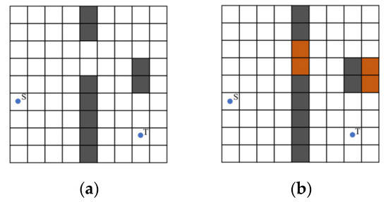
Figure 1.
Global Map and Global Map of Obstacle Gaps (a) Global Map; (b) Global Map of Obstacle Gaps.
There are two disadvantages to the original A* algorithm:
- The computing efficiency is seriously affected by too many search nodes;
- The continuity of movement is affected by redundant colinear nodes and turning points.
In response to the above problems, the following improvements are proposed in this study:
- A phenomenon in which the slow diffusion part of the search deviates from the path from the current semi-closed area to the next half-closed area is observed by visualizing the search process of the A* algorithm. And this path can be defined as the obstacle gap, deviating from this path is inconsistent with the experience of human experts.
- Based on the concept of obstacle gap, the search heuristic function, the search node direction, and the final path selection of the A* algorithm are comprehensively optimized.
The 1/6 threshold for obstacle gap identification balances robot maneuverability and environmental constraints. This ratio ensures detected gaps exceed 1.5× the robot’s width (with a safety margin) in standard 10 m × 10 m operational environments. For typical service robots (0.4–0.6 m width), this corresponds to a minimum navigable gap of 1.67 m (1/6 of 10 m), validated through simulations showing >90% traversal success while minimizing false detections. The nodes (G) are automatically tagged during map initialization (Figure 1b) to prioritize physically feasible narrow paths.
2.1.1. The Improvement of Heuristic Function
As it is difficult to judge whether the current optimal cost is a feasible path, too many edge points far from the target path will be retrieved in the search process of the A* algorithm. If the estimated value of the heuristic function is less than the actual cost value, the optimal path can be obtained, but there will be too many search nodes, which reduces the efficiency. On the contrary, if the estimated value of the heuristic function is larger than the actual cost value, it will be difficult to obtain the optimal path, but fewer nodes will be searched. And the highest search efficiency is achieved when the estimated value of the heuristic function is equal to the actual cost value.
Since the Euclidean distance is adopted by the heuristic function for judging, the role of the heuristic function at this time is only to provide the search algorithm with an estimated optimal path cost and in order to guide the search process to select the most promising nodes for expansion. However, based only on the straight-line distance between two points and ignoring the obstacles or any other constraints, the A* algorithm tends to explore the path directly connected to the target node first to speed up the search process in some cases. However, the Euclidean distance may overestimate the cost of the actual path when there are obstacles or unwalkable areas. That may cause the A* algorithm to choose to scale through the path of the obstacle instead of a longer path around the obstacle, and the resulting generated path could not meet the practical feasibility requirements. Meanwhile, more nodes may be expanded by the A* algorithm, thus increasing the computational overhead. In some cases, a more precise heuristic function may guide the search better and reduce unnecessary node expansion.
Based on the above, the Chebyshev distance is introduced in this study to provide a more accurate path cost estimation and a variable weight heuristic function is designed for the computational complexity problem to reduce the search nodes while ensuring the effectiveness of the cost of the heuristic function. The heuristic function [20] is shown as Equation (1), the Euclidean distance [21] as Equation (2), and the Chebyshev distance [22] as Equation (3).
At the same time, the weight of should be adjusted timely to improve efficiency. And the estimated value will approach the actual value gradually as the current point approaches the target. In order to increase the accuracy and reliability of the search and avoid the failure of finding the optimal path due to the excessive estimate, the estimated value is weighted also. In summary, the improved cost function is shown in Equation (4).
where, is the distance between the robot and the middle point of the obstacle gap, and is the distance between the robot and the target point.
The final design of the heuristic function for the A* algorithm is given by Equation (5), as follows:
By introducing the dynamic weighting factor , the heuristic factor can be strengthened. When the heuristic factor is too large, the shortest path may not be found. And if the heuristic factor is too small, the A* algorithm will degenerate into the Dijkstra algorithm, which takes too long. At the same time, the heuristic value of will bring negative effects when there are too many passable gaps. And only if the count of passable gaps is small, the heuristic value of can be increased to avoid searching redundant grids and enhance the efficiency of the overall pathfinding process. The specific calculation is shown in Equation (6), as follows:
where, represents the number of currently searched grids, represents the total number of gap regions, and represents the number of gap regions that have been searched. It can be obtained by the Gaussian function property that, the value of is low when the more gap regions exist in the remaining search region, and the heuristic is weak.
2.1.2. The Search Point Selection Strategy Based on Gap Optimization
The traditional A* algorithm expands the current node’s eight adjacent grid cells, represented by n1 to n8. However, in the selection of target points, although there are eight neighborhood grids to choose from, it leads to unnecessary grids, which wastes computing time and storage space. In order to further improve the search efficiency, an optimized search point selection strategy is proposed in this study. If there is a gap between the target point and the current point in the current search region, the three nearest neighbor search directions that are in line with the gap node concentration point are abandoned. By implementing the above optimization measures, the number of search nodes can be reduced, and computing efficiency can be improved. Figure 2 illustrates the search point selection strategy in this study path planning method. The left grid map shows the traditional search strategy, where the search area is limited and does not effectively consider obstacle gaps. The right grid map demonstrates our improved strategy, where the search points (marked as green squares) are selected based on gap optimization. This strategy expands the search area to better navigate through small gaps. Obstacle areas are marked in orange, and the optimal path is highlighted in yellow. This figure highlights how strategy enhances path planning by optimizing search points based on obstacle gap features.
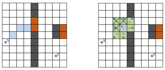
Figure 2.
Search Point Selection Strategy.
2.1.3. The Path Optimization Based on Gap Extraction
In the traditional A* path planning method that generates a path based on a grid map, the improvement of related redundant point deletion takes a long time to calculate, and the calculation of obstacle collision detection with different angles is difficult. Therefore, it does not meet the actual movement needs of robots. And the nodes are optimized by the obstacle gap map as follows:
- Extracting the gap map layer by obtaining the gap grid number of each obstacle in the global map;
- All the gap points represented by {P1, P2…Pn} passed by the robot are obtained by matching the grid matrix obtained by path planning with the gap map layer matrix. Then, put the starting and ending points into the set to generate the set of all nodes to be computed, which is represented by {Start Point, P1, P2…Pn, Target Point}. And the non-colliding node is obtained by calculating whether the neighboring path nodes of all nodes in the obtained node set. The calculation process is shown in Figure 3.
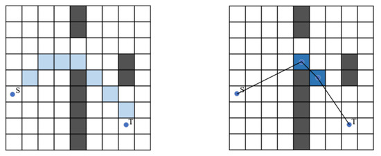 Figure 3. Node Optimization Process.
2.1.4. The Procedure of Proposed Algorithm
Step 1. The open list and close list are constructed to store the grid to be calculated and the calculated grid, respectively.
Step 2. Add the starting point to the open list and use a variable with the name of the path to compute the forward motion grid for the robot. Then, let the path equal the first element from the open list, and judge whether the path is equal to the target point. If the path is equal to the end point, the procedure is complete, otherwise, go to Step 3.
Step 3. Move the first element in the open list to the closed list, indicating that this path has been taken.
Step 4. All neighbors of the path are found and stored in a temporary variable neighbors List. Then eliminate the elements that have already been traveled in neighbors List.
Step 5. If neighbors List is not in the open list, it means that f(n) has not been calculated, calculate f(n), and set the parent node of neighbors List to path, then put it in the first place of the open list when f(n) is the smallest (ensure the shortest path).
Step 6. Recalculation of f(n) and updating f(n) and g(n) as well as the parent node if the recalculation is smaller than the previously computed value.
Step 7. Repeat Steps 2–6 until there are no elements in the open list (meaning no paths).
Step 8. If the path is successfully found, the endpoint is used to trace back to find the parent node, each parent node is stored in the pathList set, and the final set of path nodes is generated based on the path optimization method of gap extraction.
2.2. Real-Time Robot Control Method for Optimization of Clearance Angle
2.2.1. Obstacle Avoidance Angle Generation Method Based on Gap Extraction
The distance measurement between the robot and the obstacle is very important to determine the heading angle and speed of the robot during motion. The circular robot is regarded as a point robot in Cartesian space, and the distance between the robot and the obstacle boundary is calculated, represented by d. The Pythagorean theorem is used in the computational method by considering the geometry of the robot and the obstacles, as shown in Equation (7).
The heading angle of the robot is the angle adopted by the mobile robot to go to the goal position, which is an element composed of the clearance angle and the goal angle. The final heading angle of the robot is calculated based on the gap array so that the robot selects the position in the largest gap center during the motion. It is also considered that the robot may become unstable when there are multiple gaps of similar size; a suitable gap distance coefficient is used to eliminate the interference of redundant gaps. The optimal angle of each gap is deduced, and the new feasible gap is selected as the moving target of the robots. There are two key variables in the utility function: the size of the gap dn and the angle δn between the target point and the center of the gap. Which are formulated by Equation (8).
where, dn-gap and δn are, respectively, the size of the gap and the angle between the target point, and n represents the number of gaps. m1 and m2 are the weight coefficients of gap size and angle, respectively.
The gap angle between the target point and the center of the nth gap is expressed as Equation (9), as follows:
where, αn is the angle of the sampling path to the center line of the gap, and β is the angle of the current sampling path to the target point.
By considering both the size of the gap and its heading angle to the target point, the feasible gap of the robot can be calculated. And guiding the robot to choose the closest feasible gap to reach the goal position quickly, the shorter path is created while ensuring a collision-free trajectory. The optimal angle search is shown in Figure 4.
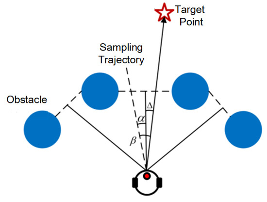
Figure 4.
Schematic diagram of optimal angle search.
At the same time, the evaluation function of the dynamic window algorithm is improved, which is shown in Equations (10) and (11), as follows:
where represents the reciprocal of the difference between the angle from the robot guidance angle to the end point and the optimal obstacle avoidance. Angle is the sample path heading angle for the robot.
2.2.2. Optimization of the Optimal Global Piecewise Control Point
The global optimal path searched by the existing algorithms is still difficult to balance the cooperativity between global planning and trajectory tracking. Therefore, it is necessary to set a virtual endpoint that has not yet reached the global path and is not within the non-navigable area by estimating the piecewise control stability. This point is usually an accurate position, but the trajectory tracking usually cannot be accurate to that point. So, it is necessary to set an appropriate threshold between the position of the robot and the point to avoid the stagnation phenomenon of the robot wandering around the point.
The stability of global path planning can be represented by the curvature of the trajectory curve. The larger the trajectory jitter is, the greater the absolute value of the trajectory curvature is. In this study, the curvature is adopted to evaluate the stability of hybrid path planning, which can account for wobble and jitter in the process of motion and represent the deviation effectively when the robot executes the global path. In the existing methods, the midpoint of the grid is used as the global path control point, which will limit the path selection of the robot and increase the collision risk of the turning angle and through the gap.
Therefore, the trajectory tracking method is adopted in this paper to introduce the robot motion model into the global path planning process and derives the following Equation (12) for the robot motion control model:
The motion of the robot with the method of the dynamic window can be regarded as an arc, and the position of the robot and the curvature of the arc can be solved by Equations (13)–(16):
The dynamic window approach models robot motion as a circular arc. Equation (12) defines the robot’s kinematic model, showing how its state evolves based on control inputs. Equations (13)–(16) are derived from this model to calculate the radius of curvature and predict the robot’s position and orientation over time. These formulas collectively enable motion prediction and path planning.
In order to further calculate the curvature and solve the optimal trajectory control points of the dynamic window method, the minimal curvature is adopted as the control objective, and each segment trajectory is fitted by the fifth-degree polynomial piecewise, which is shown in Equation (17):
The reciprocal of each order of any trajectory segment can be obtained by derivation of the above formula. In order to match the control target, each path point calculated by A* is selected as the curvature control point, and the curvature formula at t is shown in Equation (18).
The trajectory optimization problem is transformed into a quadratic programming problem with the control goal of minimizing curvature, which ensures the coupling degree and robustness of global and local paths, as shown in Equation (19):
and in order to improve the speed and quality of the trajectory solution, the parallel Bernstein equation [23] is used to solve the trajectory control points.
3. Experimental Verification
In order to verify the effectiveness and superiority of the proposed improved algorithm, a set of experiments, such as global path planning and hybrid path planning in a simulation environment, and navigation in a real environment are carried out to compare the proposed algorithm with other algorithms. In the simulations, we utilized the Robot Operating System (ROS) Noetic, installed on both the robot and a personal PC with Ubuntu 20.04. Additionally, the simulation experiments were carried out within the MATLAB environment (version R2021b).
3.1. The Simulation Experiment of Global Path Planning
In this section, a 30 × 30 grid environment is set up, and the performance of the proposed algorithm is compared with the algorithms in references [6,16].
The experimental results of scenario 1 are shown in Figure 5, and the experimental parameters are shown in Table 1. It can be seen that compared with the traditional A* algorithm, the proposed algorithm reduces the number of nodes, path length, path optimization times, and time consuming through the path optimization strategy significantly. And only a part of the redundancy points of the path are removed by the algorithm proposed by reference [16]. Compared with reference [6], although the length of the path is the same, the algorithm proposed in this study has a better comprehensive performance, and the final path generated by it is more consistent with the kinematic law of mobile robots. In addition, the key point selection range of the global method can be further optimized by the parallel Bernstein equation, which is more conducive to the subsequent selection of the local path planning range.
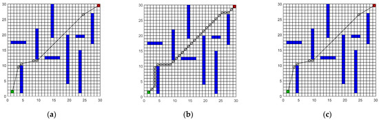
Figure 5.
Global Path Simulation Experiment for Scenario 1. (a) Algorithm from reference [6]; (b) Algorithm from reference [16]; (c) The algorithm in this paper.

Table 1.
Experimental results for Scenario 1.
The experimental results and parameters are shown in Figure 6 and Table 2. In the global search, the proposed algorithm can achieve the global optimal search without redundancy in a neutral posture. Compared with reference [5], the number of search nodes and optimization times of the proposed algorithm are significantly reduced.
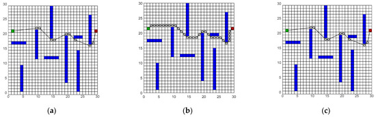
Figure 6.
Global Path Simulation Experiment for Scenario 2. (a) Algorithm from reference [6]; (b) Algorithm from reference [16]; (c) The algorithm in this paper.
Table 2.
Experimental results for Scenario 2.
3.2. The Simulation Experiment of Hybrid Path Planning
A hybrid path planning experiment is carried out, and the DWA algorithm is used to track the globally generated waypoints. The experimental results and parameters of scenario 3 are shown in Figure 7 and Table 3.
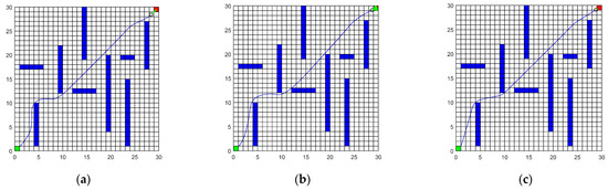
Figure 7.
Mixed Path Simulation Experiment for Scenario 3. (a) Algorithm from reference [6]; (b) Algorithm from reference [16]; (c) The algorithm in this paper.
Table 3.
Experimental results for Scenario 3.
The global control points are generated by the optimization model considering the smoothness and stability of the local path, which avoids unnecessary redundant steering and obtains the optimal local path effectively. And the improved A* algorithm can reduce the curvature to shorten the rotation time and spread the posture adjustment to the global path. However, in terms of co-directional posture, the algorithms in references [6,16] can also ensure the adjustment of the robot motion angle, which is not obvious compared with the improved A* algorithm. This can be attributed to the fact that the starting point is close to the X-axis, resulting in an insufficient path length of attitude adjustment.
Then, the experimental results and parameters of scenario 4 are shown in Figure 8 and Table 4. It can be seen that references [6,16] fail to reach the goal because the passage ability in a continuous narrow gap is weak. The classical DWA, which is adopted by them, only considers the forward motion while ignoring the influence of curvature on the passage of the robot.
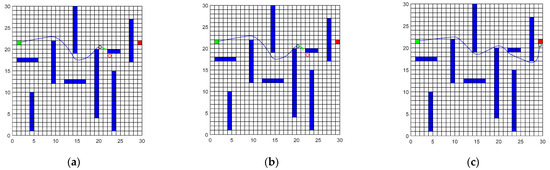
Figure 8.
Mixed Path Simulation Experiment for Scenario 4. (a) Algorithm from reference [6]; (b) Algorithm from reference [16]; (c) The algorithm in this paper.
Table 4.
Experimental results for Scenario 4.
3.3. The Experiment in the Real Environment
In this study, indoor integrated navigation experiments were conducted using the Tracer robot developed by Agile Robotics, which was equipped with an on-board laptop. The robot runs ROS Noetic on Ubuntu 20.04 and carries various sensors like a laser radar and an IMU. It navigates in a VLP-16-equipped indoor environment with complex layouts and dynamic obstacles. The on-board laptop handles real-time data processing and algorithm execution, ensuring smooth robot operation. The Agile X Tracer robot, equipped with a laptop computer, is adopted to carry out indoor integrated navigation experiments in this study. As mature robot navigation algorithms, the A* and DWA algorithms in ROS-Nav are widely used in real hybrid path planning, so they are used as comparison algorithms for the proposed improved algorithm.
Experimental scenario 1 is shown in Figure 9, which is a multi-bend scenario.
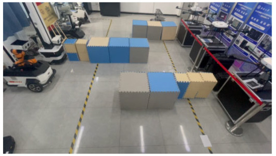
Figure 9.
Real-Machine Experiment Scenario 1.
It can be seen in Figure 9 and Figure 10 and Table 5 that since the proposed algorithm has obvious optimization in the path length, the number of turning points, and the control disturbance rate, it is significantly better than the general ROS-Nav algorithm in the actual navigation time.
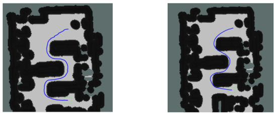
Figure 10.
Experimental comparison diagram for Scenario 1.
Table 5.
Algorithm experiment results for Scenario 1.
Experimental scenario 2 is composed of multiple narrow gap scenes. It is shown in Figure 11.
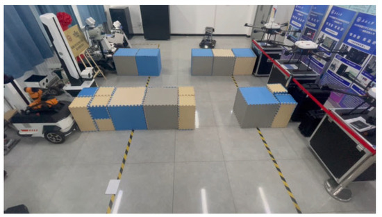
Figure 11.
Real-Machine Experiment Scenario 2.
Figure 11 and Figure 12 are the results of the navigation experiment. The trajectory angle generated by the algorithm in this study is smaller and smoother, and the attitude adjustment during the movement is more uniform, which is more suitable for the actual movement of the robot. It can be seen in Table 6 that there is a clear optimization of the movement time when the path length is close.
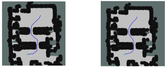
Figure 12.
Experimental comparison diagram for Scenario 2.
Table 6.
Algorithm experiment results for Scenario 2.
This work emphasizes path planning in tight spaces, distinct from the Intelligent Follow Gap Method (IFGM) presented in [24], which focuses on U- and H-shaped obstacles. While IFGM combines the Intelligent Bug Algorithm and Follow the Gap Method for goal-oriented navigation and local minima avoidance, our approach targets small gap scenarios. Both methods offer unique solutions within the mobile robot navigation field.
4. Conclusions
This paper examines the crucial issue of global path planning and stable tracking for mobile robots in extensive settings. A novel hybrid planning algorithm is proposed, merging an enhanced safe A* algorithm for global path planning with sophisticated motion planning algorithms for path tracking. This innovative approach ensures real-time navigation capabilities while markedly improving path accuracy and obstacle avoidance. The enhancement of the A* algorithm through optimized risk assessment in the cost function reduces computational load and accelerates decision-making. Furthermore, the hybrid strategy utilizes a real-time motion planning method with an adaptive window mechanism, enabling dynamic extraction and switching of critical path points as sub-targets to ensure smooth and collision-free path tracking. This combination of techniques results in significantly enhanced navigation efficiency and reliability in complex environments.
(1) The heuristic function was constructed by the influence of the gap units extracted from the global grid map on the global path planning. And the global path generated at the gap points was optimized to reduce the redundant nodes.
(2) The best steering angle of the robot through the obstacles was calculated by considering the position relationship between the obstacles. And the robustness and success rate of navigation were improved by adding an obstacle gap angle function to the dynamic window path evaluation function, which could change the moving direction of the mobile robots.
(3) The robot kinematics model was introduced in the process of optimizing the global path, which ensured that the setting of each virtual sub endpoint was more in line with the motion constraints, the posture adjustment was more reasonable, and the time consumed of local path planning was shorter.
(4) The experimental results showed that the proposed algorithm has a higher computational efficiency and faster optimization speed in the global static maps. And the effectiveness and robustness of mobile robot navigation were improved by the segmented virtual endpoint calculation methods of the dynamic window method. It was superior to the references [6,16] in terms of safety and motion performance in simulation and the real environment.
(5) Future work will focus on collision-free local path planning algorithms that take into account the velocity of mobile robots. And the noise and uncertainty of robots will also be taken into account precisely to create a more extensive, fast, and safe path planning algorithm.
Author Contributions
Conceptualization, H.W. and L.H.; methodology, H.W. and L.H.; software, S.Z.; formal analysis, S.Z.; investigation, R.B. and Y.W.; resources, H.W.; data curation, Y.W. and R.B.; writing—original draft preparation, H.W.; writing—review and editing, L.H.; visualization, S.Z.; supervision, H.W.; project administration, H.W.; funding acquisition, H.W. All authors have read and agreed to the published version of the manuscript.
Funding
This work was supported by the Natural Science Foundation of Xinjiang Uygur Autonomous Region (2022D01C392); the Xinjiang Uygur Autonomous Region Key Research and Development Project (2022B02016-1).
Institutional Review Board Statement
Not applicable.
Informed Consent Statement
Not applicable.
Data Availability Statement
The data presented in this study are available on request from the corresponding author. The data are not publicly available due to privacy concerns.
Conflicts of Interest
The authors declare no conflicts of interest.
References
- Li, C.G.; Huang, X.; Ding, J.; Song, K.; Lu, S.Q. Global path planning based on a bidirectional alternating search A* algorithm for mobile robots. Comput. Ind. Eng. 2022, 168, 108123. [Google Scholar] [CrossRef]
- Hassan, M.U.; Ullah, M.; Iqbal, J. Towards autonomy in agriculture: Design and prototyping of a robotic vehicle with seed selector. In Proceedings of the 2016 2nd International Conference on Robotics and Artificial Intelligence (ICRAI), Rawalpindi, Pakistan, 1–2 November 2016; pp. 37–44. [Google Scholar]
- Wang, C.Q.; Chen, X.Y.; Li, C.M.; Song, R.; Li, Y.B.; Meng, M.Q.H. Chase and Track: Toward Safe and Smooth Trajectory Planning for Robotic Navigation in Dynamic Environments. IEEE Trans. Ind. Electron. 2023, 70, 604–613. [Google Scholar] [CrossRef]
- Fu, B.; Chen, L.; Zhou, Y.T.; Zheng, D.; Wei, Z.Q.; Dai, J.; Pan, H.H. An improved A* algorithm for the industrial robot path planning with high success rate and short length. Robot. Auton. Syst. 2018, 106, 26–37. [Google Scholar] [CrossRef]
- Alshammrei, S.; Boubaker, S.; Kolsi, L. Improved Dijkstra Algorithm for Mobile Robot Path Planning and Obstacle Avoidance. CMC—Comput. Mater. Contin. 2022, 72, 5939–5954. [Google Scholar] [CrossRef]
- Cheng, C.; Hao, X.; Li, J.; Zhang, Z.; Sun, G. Global dynamic path planning based on fusion of improved A* algorithm and dynamic window approach. J. Xi’an Jiaotong Univ. 2017, 51, 137–143. [Google Scholar]
- Wang, H.W.; Lou, S.J.; Jing, J.; Wang, Y.S.; Liu, W.; Liu, T.M. The EBS-A* algorithm: An improved A* algorithm for path planning. PLoS ONE 2022, 17, e026384. [Google Scholar] [CrossRef]
- Liu, Y.J.; Wang, C.; Wu, H.; Wei, Y.L. Mobile Robot Path Planning Based on Kinematically Constrained A-Star Algorithm and DWA Fusion Algorithm. Mathematics 2023, 11, 4552. [Google Scholar] [CrossRef]
- Zhong, X.Y.; Tian, J.; Hu, H.S.; Peng, X.F. Hybrid Path Planning Based on Safe A* Algorithm and Adaptive Window Approach for Mobile Robot in Large-Scale Dynamic Environment. Intell. Robot. Syst. 2020, 99, 65–77. [Google Scholar] [CrossRef]
- Chi, Z.Z.; Yu, Z.H.; Wei, Q.Y.; He, Q.C.; Li, G.X.; Ding, S.L. High-Efficiency Navigation of Nonholonomic Mobile Robots Based on Improved Hybrid A* Algorithm. Appl. Sci. 2023, 13, 6141. [Google Scholar] [CrossRef]
- Huang, C.S.; Zhao, Y.P.; Zhang, M.J.; Yang, H.Y. APSO: An A*-PSO Hybrid Algorithm for Mobile Robot Path Planning. IEEE Access 2023, 11, 43238–43256. [Google Scholar] [CrossRef]
- Liu, L.X.; Wang, X.; Yang, X.; Liu, H.J.; Li, J.P.; Wang, P.F. Path planning techniques for mobile robots: Review and prospect. Expert Syst. Appl. 2023, 227, 120254. [Google Scholar] [CrossRef]
- Wu, L.; Huang, X.D.; Cui, J.G.; Liu, C.; Xiao, W.S. Modified adaptive ant colony optimization algorithm and its application for solving path planning of mobile robot. Expert Syst. Appl. 2023, 215, 119410. [Google Scholar] [CrossRef]
- Zou, A.; Wang, L.; Li, W.M.; Cai, J.C.; Wang, H.; Tan, T.L. Mobile robot path planning using improved mayfly optimization algorithm and dynamic window approach. J. Supercomput. 2023, 79, 8340–8367. [Google Scholar] [CrossRef]
- Zhang, D.; Luo, R.; Yin, Y.B.; Zou, S.L. Multi-objective path planning for mobile robot in nuclear accident environment based on improved ant colony optimization with modified A. Nucl. Eng. Technol. 2023, 55, 1838–1854. [Google Scholar] [CrossRef]
- Lao, C.; Li, P.; Feng, Y. Path Planning of Greenhouse Robot Based on Fusion of Improved A* Algorithm and Dynamic Window Approach. J. Agric. Mach. 2021, 52, 14–22. [Google Scholar]
- Liao, T.J.; Chen, F.; Wu, Y.T.; Zeng, H.Q.; Ouyang, S.J.; Guan, J.S. Research on Path Planning with the Integration of Adaptive A-Star Algorithm and Improved Dynamic Window Approach. Electronics 2024, 13, 455. [Google Scholar] [CrossRef]
- Li, Y.G.; Jin, R.C.; Xu, X.R.; Qian, Y.D.; Wang, H.Y.; Xu, S.S.; Wang, Z.X. A Mobile Robot Path Planning Algorithm Based on Improved A* Algorithm and Dynamic Window Approach. IEEE Access 2022, 10, 57736–57747. [Google Scholar] [CrossRef]
- Zohaib, M.; Pasha, S.M.; Javaid, N.; Iqbal, J. IBA: Intelligent Bug Algorithm—A Novel Strategy to Navigate Mobile Robots Autonomously. Commun. Comput. Inf. Sci. 2014, 414, 291–299. [Google Scholar]
- Wang, P.Y.; Liu, Y.L.; Yao, W.M.; Yu, Y. B; Improved A-star algorithm based on multivariate fusion heuristic function for autonomous driving path planning. Proc. Inst. Mech. Eng. Part. D—J. Automob. Eng. 2023, 237, 1527–1542. [Google Scholar] [CrossRef]
- Bai, R.Y.; Wang, H.W.; Sun, W.L.; He, L.; Shi, Y.X.; Xu, Q.G.; Wang, Y.H.; Chen, X.C. Intelligent diagnosis of gearbox in data heterogeneous environments based on federated supervised contrastive learning framework. Sci. Rep. 2025, 15, 14596. [Google Scholar] [CrossRef]
- Liu, X.; Chen, W.T.; Peng, L.; Luo, D.; Jia, L.K.; Xu, G.; Chen, X.B.; Liu, X.M. Secure computation protocol of Chebyshev distance under the malicious model. Sci. Rep. 2024, 14, 17115. [Google Scholar] [CrossRef] [PubMed]
- Kousik, S.; Zhang, B.; Zhao, P.; Vasudevan, R. Safe, Optimal, Real-Time Trajectory Planning with a Parallel Constrained Bernstein Algorithm. IEEE Trans. Robot. 2021, 37, 815–830. [Google Scholar] [CrossRef]
- Zohaib, M.; Pasha, S.M.; Javaid, N.; Salaam, A.; Iqbal, J. An improved algorithm for collision avoidance in environments having U and H shaped obstacles. Stud. Inform. Control 2014, 23, 97–106. [Google Scholar] [CrossRef]
Disclaimer/Publisher’s Note: The statements, opinions and data contained in all publications are solely those of the individual author(s) and contributor(s) and not of MDPI and/or the editor(s). MDPI and/or the editor(s) disclaim responsibility for any injury to people or property resulting from any ideas, methods, instructions or products referred to in the content. |
© 2025 by the authors. Licensee MDPI, Basel, Switzerland. This article is an open access article distributed under the terms and conditions of the Creative Commons Attribution (CC BY) license (https://creativecommons.org/licenses/by/4.0/).