Hyperband-Optimized CNN-BiLSTM with Attention Mechanism for Corporate Financial Distress Prediction

Abstract

In the context of new quality productive forces, enterprises must leverage technological innovation and intelligent management to enhance financial risk resilience. This article proposes a financial distress prediction model based on deep learning, combined with a CNN, BiLSTM, and attention mechanism, using SMOTE for sample imbalance and Hyperband for hyperparameter optimization. Among four CNN-BiLSTM-AT model structures and seven mainstream models (CNN, BiLSTM, CNN-BiLSTM, CNN-AT, BiLSTM-AT, CNN-GRU, and Transformer), the 1CNN-1BiLSTM-AT model achieved the highest validation accuracy and relatively faster training speed. We conducted 100 repeated experiments using data from two companies, with validation on 2025 data, confirming the model’s stability and effectiveness in real-world scenarios. This article lays a solid empirical foundation for further optimization of financial distress warning models.

1. Introduction

Against the backdrop of continued global economic uncertainty and the accelerated digital transformation of Chinese industries, enterprise financial risk management is facing severe challenges. According to a report by the United Nations, the global economic growth rate is expected to drop from 2.9% in 2024 to 2.4% in 2025. The global economy is recovering sluggishly, and domestic development is also under tremendous pressure. Some listed companies are facing greater operational challenges, with 29 entering bankruptcy and restructuring proceedings in 2024. This represents a 16% increase on the 25 companies in 2023, highlighting the vulnerability of enterprises’ risk resistance capacity. In this situation, the requirement for financial distress prediction to be both timely and accurate has significantly increased. However, traditional methods have a limited ability to identify nonlinear relationships and time dependence, making it difficult to respond effectively to the current complex risk characteristics.Therefore, this paper proposes a fusion model combining a convolutional neural network (CNN), a bidirectional long short-term memory (BiLSTM) network, and an attention mechanism (AT) with a Hyperband algorithm for hyperparameter optimization. The aim is to construct a dynamic warning system that is both highly precise and robust.

This article proposes a deep learning model that incorporates a CNN, a BiLSTM, and an attention mechanism. This model achieves a prediction accuracy of 0.994 on the test set, outperforming existing mainstream models. The model effectively combines CNN’s local feature extraction capability, BiLSTM’s time series modeling advantage and the attention mechanism’s dynamic weighting of key features. It also introduces the SMOTE algorithm to mitigate the bias caused by sample category imbalance, improving the recognition of distressed enterprises. The Hyperband algorithm automatically optimizes the model’s hyperparameter configuration, enhancing its overall performance and training efficiency. The model has high practical value and application potential in the early warning of financial risk and decision-making.

This article enriches the theoretical framework for predicting financial risk, deepens our understanding of the dynamic allocation of temporal features and weights of key variables in deep neural network models, and encourages the exploration of applying the attention mechanism to analyze financial data. The introduction of an automated hyperparameter optimization method improves the efficiency and generalization ability of model training and reduces the subjectivity of manual parameter tuning. Meanwhile, validation based on repeated case company trials and the latest 2025 data enhances the model’s robustness and applicability, providing more solid empirical support for financial risk management theory and laying the methodological groundwork for subsequent related research.

This article is structured as follows: Section 1 is the introduction section, outlining the research background, significance, and main contributions; Section 2 is the literature review section, reviewing the research progress in financial distress prediction and deep learning modeling at home and abroad; Section 3 is the methodology section, describing the structural design and hyperparameter optimization strategy of the proposed model; Section 4 is the experimental section, which describes the data sources, preprocessing procedure and experimental protocol; Section 5 is the results section, which covers the performance evaluation of the model structure, comparative analysis with mainstream models, and stability validation; and Section 6 is the conclusion section, which summarizes the research results, discusses the limitations, and proposes the future research direction.

2. Literature Review

In recent years, many innovative algorithms and model architectures have emerged in deep learning as data storage capacity and computational power have increased dramatically. Deep neural network architectures enable models to automatically learn hierarchical feature representations that are better adapted to real-world diversity and change. This capability has led to significant advances in image recognition, time series prediction, natural language processing, and speech recognition. They have surpassed traditional machine learning approaches in many areas. Deep learning models have significant advantages in dealing with complex nonlinear relationships and large-scale data.

Kuen (2015) applied deep learning to invariant representation learning for visual tracking, achieving good results in tracking visual descriptions through strong spatiotemporal constraints and stacked convolutional autoencoders [1]. Gu et al. (2020) compared various machine learning methods for asset risk premium prediction and found that models like neural networks significantly outperform traditional regression-based approaches [2]. HHosaka (2019) selected financial ratios from financial statements of four fiscal periods and attempted to generate images for training and testing automatically. A convolutional neural network model for bankruptcy prediction was constructed and compared with various methods such as Z-Score, decision tree, support vector machine, linear discriminant analysis, AdaBoost, etc. The results showed that the convolutional neural network had better predictive performance [3]. Zhou et al. (2023) showed that deep neural network models outperform ordinary least squares and historical average methods in forecasting the equity premium [4]. Li (2021) used Google’s “Bert-based Chinese” pre-trained language model to represent word vectors and combined the advantages of a bidirectional recurrent neural network (BiRNN) and LSTM to construct the BiLSTM model. This deep learning-based model can achieve high predictive performance in four aspects of emotions: the capital market, the stock market, the internal conditions of enterprises, and politics [5]. Aslam et al. (2021) proposed an LSTM model for predicting stock market reactions to sudden events such as terrorist attacks and natural disasters [6]. Siami-Namini compared the performance of BiLSTM and conventional LSTM in time series prediction. Research has shown that, although BiLSTM provided additional training capabilities through bidirectional traversal of input data, resulting in better prediction accuracy than unidirectional LSTM and ARIMA models, its convergence speed was slower than that of LSTM. This indicated that, although additional training can improve prediction performance, the convergence efficiency of the model also needs to be considered [7]. Tao Lihong (2022) used the Transformer model for enterprise financial crisis warning, with an accuracy rate of 92%. It should be noted that the Transformer model is essentially an attention-based model, which gives it significant advantages in capturing key features and relationships in data [8]. The application of deep learning models in financial early warning is quite significant.

Many scholars have begun constructing composite models to improve individual models’ performance and prediction accuracy by integrating the advantages of multiple models. Ouyang (2021) constructed a risk warning model using an attention-LSTM neural network and found that, compared with the BP neural network model, the SVM model, and the ARIMA model, the attention-LSTM neural network had higher average prediction accuracy in the short, medium, and long term [9]. Zhao Y (2023) proposed a financial crisis prediction model with a feature attention mechanism based on an artificial bee colony recurrent neural network (ABC-RNN) and bidirectional long short-term memory (BiLSTM), with an accuracy of 89% [10]. Chen (2024) proposed a hybrid model, TG-LSTM, which combines time series ratio analysis and a long short-term memory (LSTM) model, and improves prediction accuracy through TSVD technology and the XGBoost method. When the data dimension was reduced, experimental results show that the model’s accuracy on the CSI 300 and SSE 50 datasets reached 96.1%, significantly better than traditional methods [11]. In addition, deep learning has also been widely applied in other fields. The CNN-BiLSTM model, combined with the attention mechanism proposed by Lu et al. (2021), performed the best in predicting stock prices in practical applications [12]. Kavianpour (2023) combined convolutional neural networks (CNNs), bidirectional long short-term memory (BiLSTM) networks, attention mechanisms, and zero-order preservation (ZOH) preprocessing techniques to predict the maximum magnitude and number of earthquakes in the following month. Through evaluating earthquake data from nine regions in China, the results showed that this method outperforms other prediction methods (SVM, MLP, DT, RF, CNN, LSTM, and CNN-BiLSTM) in terms of performance and generalization ability [13]. Han et al. (2025) proposed a generalized multimodal fusion approach (MFB) for Bitcoin price prediction by integrating time-lagged sentiment signals from news and tweets with technical indicators. Their model combines BiLSTM and BiGRU layers for deep feature extraction, utilizes BorutaShap for feature selection, and applies attention mechanisms and spatial dropout for improved generalization [14]. Chen Jian and Liu Weiji (2023) used Hyperband-LSTM to predict stock prices, and the results showed that using the Hyperband algorithm to optimize hyperparameters yielded better and more robust results than the Bayes algorithm [15]. This indicates that deep learning methods can significantly improve the predictive ability of time series data.

Although deep learning has made some progress in the prediction of financial distress, most of the existing research focuses on the prediction of price trends or the modeling of market reactions based on unexpected events, such as the use of sentiment analysis, multimodal fusion, or the prediction of unstructured textual data, and the research of in-depth modeling for structured financial data is still relatively limited. At the same time, existing studies are still deficient in terms of model interpretability and applicability, and often lack in-depth analyses of the internal mechanisms of models, making it difficult to meet the demand for transparency and reliability in financial decision-making. In particular, the structural design and selection of hyperparameters of combined models are not yet sufficiently applied in the field of financial risk identification, and there is a lack of systematic performance comparisons and mechanism analyses. To address these issues, this article proposes a combined model that integrates a Hyperband algorithm, a convolutional neural network (CNN), bidirectional long short-term memory (BiLSTM), and an attention mechanism (AT) for financial distress prediction. This model improves the interpretability and effectiveness of the model by optimizing the combination structure and hyperparameter selection, combined with ablation methods and company case applications, and further enhances the ability to mine temporal features, thereby promoting the application of deep learning technology in the financial field.

3. Methodology

3.1. CNN-BiLSTM-AT

CNNs can extract local salient features from a company’s financial data through convolutional layers. BiLSTM can capture bidirectional dependencies in the time series, and, by adding a bidirectional LSTM layer on top of the features extracted by the CNN, the performance of the company’s financial metrics for each quarter before financial distress can be learned. The attention mechanism (AT) can identify key features in the financial data of each quarter and add these features to the output results after weighting them to improve the model’s performance. Based on these features, the development of a CNN-BiLSTM-AT model for financial risk prediction is reported in this article. The structure of the model is shown in Figure 1, and mainly includes an input layer, a CNN layer, a BiLSTM layer, an attention mechanism layer, two fully connected layers, and an output layer.

The model processes a series of consecutive financial indicators from multiple quarters with an input tensor shape of (batch_size, time_steps, features), where time_steps represents the continuous time steps in each sample. The convolutional layer extracts local patterns along the feature dimension, while keeping the time dimension intact, resulting in an output shape of (batch_size, time_steps, filters). Max pooling is then applied to compress the time dimension, producing an intermediate representation of (batch_size, time_steps/pool_size, filters). This reduces the computational burden while preserving essential information. The pooled sequence is passed into a BiLSTM layer, which models the temporal dependencies of financial indicators bidirectionally, outputting a shape of (batch_size, time_steps/pool_size, 2 × lstm_units). An attention mechanism is used to weight and integrate time step information, generating contextual representations that emphasize key features. Finally, the model applies feature transformation through two fully connected layers, resulting in output shapes of (batch_size, dense_units_1) and (batch_size, dense_units_2). The sigmoid activated output layer then predicts the financial risk of the enterprise, with an output of (batch_size, 1). This approach combines convolutional feature extraction, cyclic time series modeling, and attention to focus on critical information, enhancing the accuracy and robustness of financial risk identification.

3.2. CNN

The CNN (convolutional neural network) was proposed by Kunihiko Fukushima in 1980, who introduced the concept of hierarchical structure and local connectivity, and something that is good at dealing with data with a grid structure [16]. Yann LeCun et al. in 1998 described in detail the structure of convolutional neural networks (CNNs) and the application of handwritten digit recognition, which contains convolutional, pooling, and fully connected layers, etc., as well as how to use the backpropagation algorithm for training and prediction [17].

(1)

The convolutional layer operation extracts the local features of the input data $x_{i+m-1,j+n-1}$ by convolution operation, i.e., the convolution kernel sliding dot product operation on the input data.

$$h_{ij}=f(\sum _{m=1}^M\sum _{n=1}^N{x}_{i+m-1,j+n-1}·w_{m,n}+b),$$

(1)

where $h_{ij}$ is the output of the convolutional layer, $x_{i+m-1,j+n-1}$ is the input data, $w_{m,n}$ is the weight of the convolutional kernel, b is the bias of the convolutional kernel, and f is the $ReLU$ activation function.

(2)

Pooling layer operation uses a maximum pooling operation to divide the input data into non-overlapping rectangular regions. It selects the maximum value within each rectangular region as the representative value for that region.

$$p_{ij}=max\left(h_{2i,2j},h_{2i,2j+1},h_{2i+1,2j},h_{2i+1,2j+1}\right)$$

(2)

where the above formula is for a maximum pooling window of 2 × 2 and a step size of 2, indicating the value of the position in the output region after the pooling operation.

(3)

Fully connected layer operations, where the multi-dimensional feature maps output from the convolutional or pooling layers are spread into one-dimensional vectors and fed into one or more fully connected layers, and the classification results are outputted using the softmax activation function.

$$y_k=\sigma (\sum _{i=1}^N{w}_{k,i}·p_i+b_k),$$

(3)

where $w_{k,i}$ is the weight of the fully connected layer, $p_i$ is the output of the last pooling layer, $b_k$ is the bias of the fully connected layer, and $\sigma$ is the activation function.

3.3. BiLSTM

The BiLSTM (bidirectional long short-term memory) network was proposed by Felix A. Gers, Jürgen Schmidhuber, and Fred Cummins in 1997 as an extension of the long short-term memory (LSTM) time network. BiLSTM combines two LSTM networks that process sequences in a forward manner and a reverse manner, respectively, and this bidirectional architecture is capable of capturing the backward and forward dependencies of time series data well. BiLSTM demonstrates improved performance in many tasks by learning from past and future data, rather than solely from past data [18].

The LSTM unit is composed of input gates, output gates, forgetting gates, and memory units that can process and preserve the long-term dependencies of the time series [19].

The forgetting gate, $f_t$, controls the effect of the previous moment memory cell, $C_{t-1}$, on the current moment, i.e., the information that is unimportant in the previous and current moments can be selectively forgotten; the input gate, $i_t$, controls the effect of the input information, $x_t$, in the current moment on the memory cell, deciding which information will be stored in the memory cell, and the candidate memory cell, $\widetilde{C_t}$, combines the output, $h_{t-1}$, of the hidden layer in the previous moment, and the input information, $x_t$, in the current moment to update the new information in the current moment, and the output gate controls how much information is to be output to the hidden layer. Updating the information of the current moment memory cell, $C_t$, combines the forgetting gate and input gate, combining the memory cell, $C_{t-1}$, of the previous moment and the new information, $\widetilde{C_t}$, of the current moment; the output gate, $o_t$, controls how much information in the memory cell state, C, needs to be output to the hidden layer, H. The specific formulae are as follows.

$$h_t=\sigma (w_f·[h_{t-1},x_t]+b_f),$$

(4)

$$i_t=\sigma (w_i·[h_{t-1},x_t]+b_i),$$

(5)

$$\widetilde{C_t}=tanh(w_c·[h_{t-1},x_t]+b_c),$$

(6)

$$C_t=f_t·C_{t-1}+i_t·\widetilde{C_t},$$

(7)

$$o_t=\sigma (w_o·[h_{t-1},x_t]+b_o),$$

(8)

$$h_t=o_t·tanh\left(C_t\right)$$

(9)

where $w_f$, $w_i$, $w_c$, $w_o$ represent the weight matrices of the forgetting gate, the input gate, the candidate memory unit, and the output gate, respectively, $b_f$, $b_i$, $b_c$, $b_o$ represent the biases of the forgetting gate, the input gate, the candidate memory unit, and the output gate, respectively, and $\sigma$ are sigmoid activation functions with outputs ranging between 0 and 1, and are hyperbolic tangent functions with outputs ranging between −1 and 1.

BiLSTM combines two LSTM networks to comprehensively capture the dependencies of the sequence data by processing the sequences in both forward and reverse directions.

(1)

Positive $LSTM$ processing sequence. The input sequence is processed step by step from the first to the last time step. For each time step, t, the positive hidden layer state, $\overrightarrow{h_t}$, is computed according to the positive $LSTM$ formula.

$$\overrightarrow{h_t}=LSTM(x_t,\overrightarrow{h_{t-1}},\overrightarrow{C_{t-1}})$$

(10)

(2)

The reverse $LSTM$ processes the sequence. The input sequence is processed step by step from the last time step to the first-time step. For each time step, t, the reverse hidden layer state, $\overleftarrow{h_t}$, is computed according to the reverse $LSTM$ formula.

$$\overleftarrow{h_t}=LSTM(x_t,\overleftarrow{h_{t-1}},\overleftarrow{C_{t-1}}))$$

(11)

(3)

Connect the forward and backward hidden states. For each time step t, the forward and backward hidden states are concatenated. The concatenated hidden state $h_t$ is then passed through the fully connected layer to produce the final output $y_t$.

$$h_t=[\overrightarrow{h_t},\overleftarrow{h_t}]$$

(12)

$$y_t=\sigma (w·h_t+b)$$

(13)

3.4. Attention Mechanism

The attention mechanism (AT) was proposed by Bahdanau et al. in 2014 [20]. It was initially intended to be used mainly to improve machine translation performance by allowing the model to dynamically select and learn the relevant information in the original sentence as it translates each word, instead of relying on a fixed context vector. Unlike BiLSTM, the attention mechanism not only focuses on the input of the current time step when processing each time step of the input sequence, but also adjusts its weights based on the information of other time steps, to better capture the important information in the input sequence. In the work reported in this article, we implemented a customized layer based on additive attention.

(1)

Calculating the attention score. For each time step t, the attention score $s_t$ is calculated via the $tanh$ activation function.

$$s_t=tanh(w·h_t+b)$$

(14)

(2)

Calculating the attention weights. For each time step t, calculate the attention weights, $a_t$, using the softmax function; these weights represent the importance of each time step.

$$a_t={\displaystyle \frac{exp\left(s_t\right)}{{\sum }_{k=1}^{T}exp\left(s_k\right)}},$$

(15)

(3)

Calculating the weighted summation. Based on the calculated attention weights $a_{t,i}$, for the i-th hidden state $h_i$, at time step t, the input sequence $h_i$, is weighted and summed to obtain the context vector $c_t$ of the output of the current time step.

$$c_t=\sum _{i=1}^T{a}_{t,i}{h}_i.$$

(16)

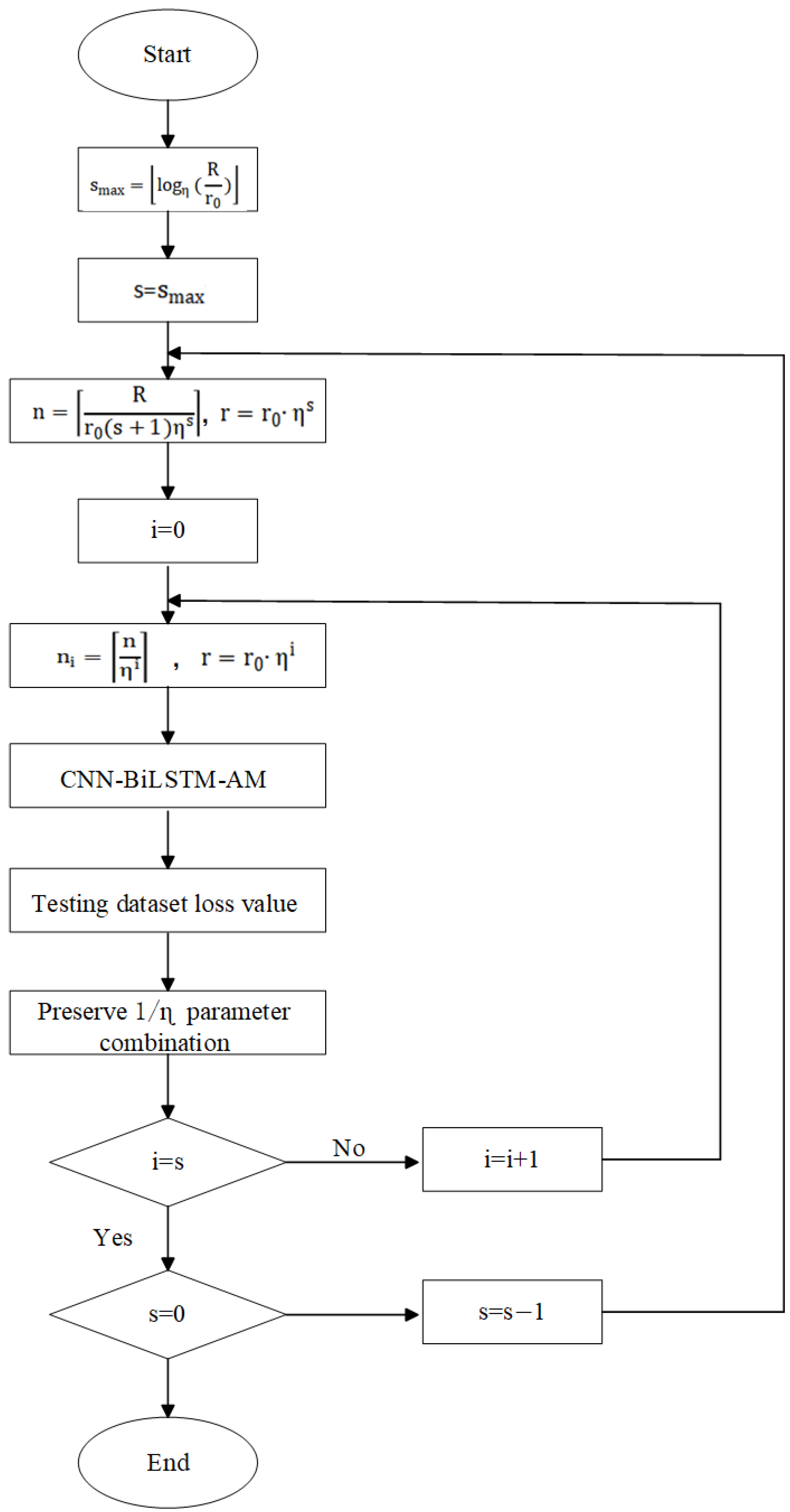
3.5. Hyperband Algorithm

The Hyperband algorithm, proposed by Lisha Li and Kevin Jamieson in 2016 [21], eliminates the underperforming hyperparameter configurations in each round by combining the Successive Halving algorithm in the multi-armed bandit strategy and efficiently selects the best-performing hyperparameter configurations from the final configuration to optimize the model training process.

(1)

Initialization parameters. Set the resource budget R (the total number of training rounds), set the bandwidth factor $\eta$ (a parameter controlling the elimination speed of hyper-parameter configurations; the default is 3), and set the initial amount of resources $r_0$ (the amount of resources used by each configuration in the initial evaluation).

(2)

Calculate maximum rounds. $s_{max}$ is the maximum number of rounds that can be performed with the current resource budget R, and initial resource amount $r_0$.

$$s_{max}=\lfloor lo{g}_{\eta }{\displaystyle \frac{R}{r_0}}\rfloor .$$

(17)

where $\lfloor \rfloor$ stands for the downward rounding sign.

(3)

Perform multiple rounds of hyperparameter configuration and the elimination process. Multiple rounds are performed from $s=0$ to $s=max$.

For each round s, the number of configurations and the amount of resources are initialized, and n hyperparameter configurations are generated, each of which receives a training resource amount r, at the beginning.

$$n=\lceil {\displaystyle \frac{R}{r_0(s+1){\eta }^s}}\rceil ,r=r_0·{\eta }^s.$$

(18)

In each round s, obtain the number of hyperparameter configurations $n_i$, and the amount of resources $r_i$, used for each configuration in the ith subphase (from 0 to s).

$$n_i=\lceil {\displaystyle \frac{n}{{\eta }^i}}\rceil ,r=r_0·{\eta }^i.$$

(19)

Allocate resources evenly to all hyperparameter configurations and perform initial training. According to the Successive Halving algorithm, eliminate the underperforming configurations and concentrate the resources on the best-performing configurations, at which point the elimination ratio is $1-{\displaystyle \frac{1}{\eta }}$, and the best-performing ${\displaystyle \frac{1}{\eta }}$ configurations are retained.

(4)

Selection of the optimal configuration. At the end of all rounds, the best-performing hyperparameter configuration is selected from the final configuration.

The Hyperband CNN-BiLSTM-AT Flowchart is shown in Figure 2.

4. Experiment

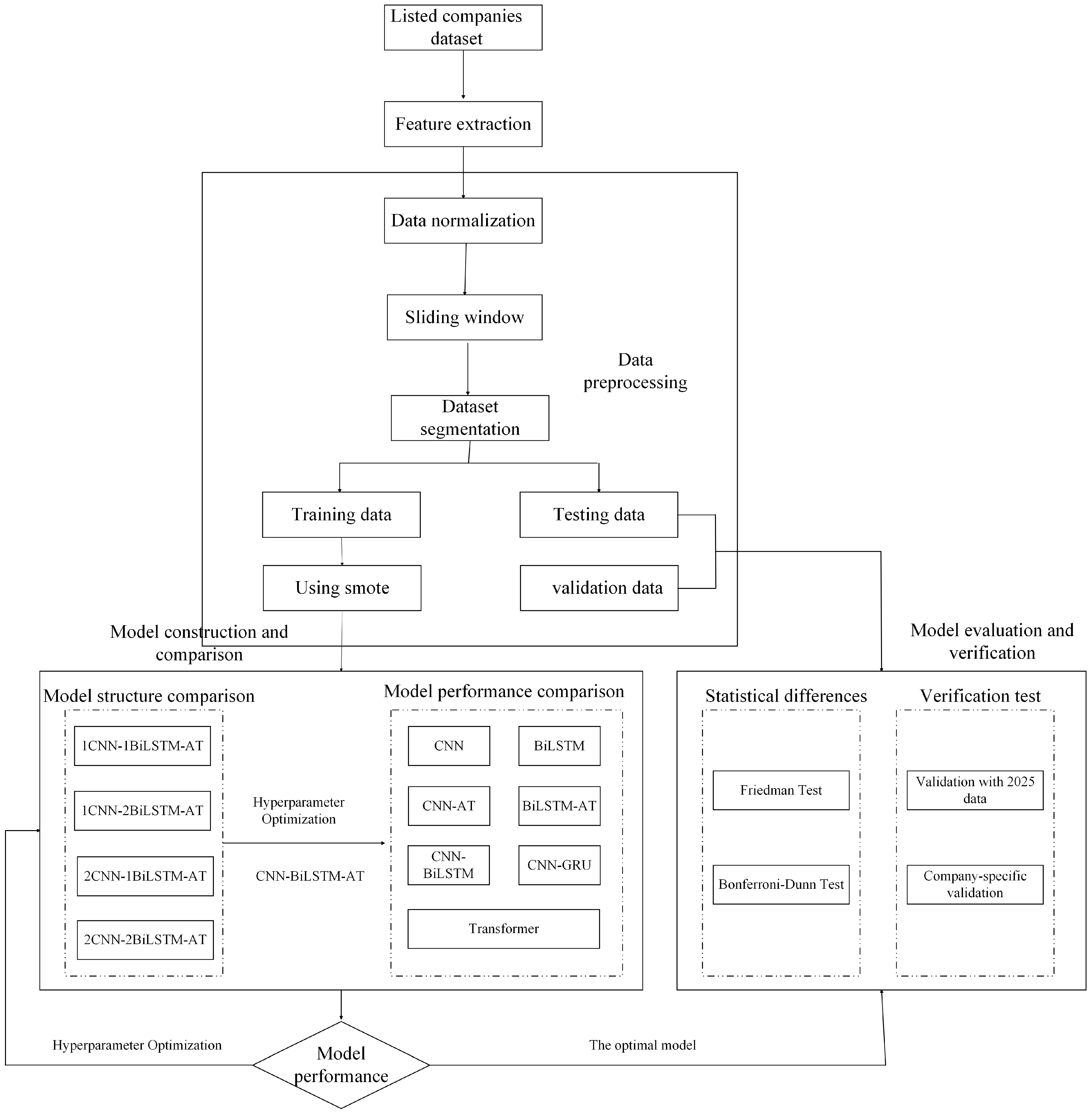
4.1. Overview of Experimental Process

The CNN-BiLSTM-AT model constructed in this study mainly predicts financial risks for listed companies. The experimental process is shown in the figure below. It can be divided into three stages: data preprocessing, model construction and training, and model prediction and evaluation. The overall workflow is illustrated in Figure 3.

In the data preprocessing stage, we first import the dataset containing financial indicators and risk labels. To eliminate the dimensional differences between different financial indicators, we use the z-score normalization method to standardize the input data. Subsequently, the standardized data are converted into time series format using a sliding window method to capture the temporal characteristics of financial indicators. Assuming a sliding window size of w, for the input data $Z=[z_1,z_2,\dots ,z_n]$, generate new data $Z^{\prime }=\left\{[z_i,z_{i+1},\dots ,z_{i+w-1}]|i=1,2,\dots ,n-w+1\right\}$. The new generated dataset is partitioned into training and test sets in a 80:20 ratio. To deal with the problem of risk category imbalance, SMOTE (a synthetic minority class oversampling technique) is used to generate new minority class samples to make the dataset more balanced; for the minority class sample, $z_i$, its nearest neighbor samples, k, are selected to generate a new sample, $z_{new}$ [22].

In the model construction and training stage, a one-dimensional convolutional neural network (CNN) is used to extract local temporal features, and the dimension is reduced through the maximum pooling operation to obtain the key feature representation; then the CNN output is passed to the bidirectional long short-term memory (BiLSTM) network to capture the temporal relationship between the front and back in the sequence; then the attention mechanism (attention layer) is introduced to give different weights to the BiLSTM output to highlight the key information. The model’s hyperparameters (including learning rate, batch size, convolution kernel size, number of LSTM units, dropout rate, number of hidden layer units, etc.) are automatically searched and optimized through the Hyperband algorithm, and the optimal configuration is finally determined to improve the model’s performance. In the model comparison stage, multiple deep learning architectures combining CNN, BiLSTM, and attention mechanism are designed, such as 1CNN-1BiLSTM-AT, 1CNN-2BiLSTM-AT, 2CNN-1BiLSTM-AT, and 2CNN-2BiLSTM-AT, and the optimal structure is determined through hyperparameter optimization. At the same time, the performance of traditional deep learning models (CNN, BiLSTM), hybrid models (CNN-AT, BiLSTM-AT, CNN-BiLSTM, CNN-GRU), and Transformer models are evaluated, and the optimal model is found by comparing the performance of each model.

In the model prediction and evaluation stage of the model, the preprocessed test data are input into the trained CNN-BiLSTM-AT model to obtain the prediction results. To ensure statistical reliability and generalizability of the results, the Friedman test and Bonferroni–Dunn follow-up test are used to assess whether the performance differences between the models are statistically significant. In the validation test phase, two types of validation are performed: one is future prediction validation using 2025 data to evaluate the temporal generalizability of the model; the other is validation of 100 repeated experiments of the company using data from two different companies to evaluate the adaptability of the model in a business environment.

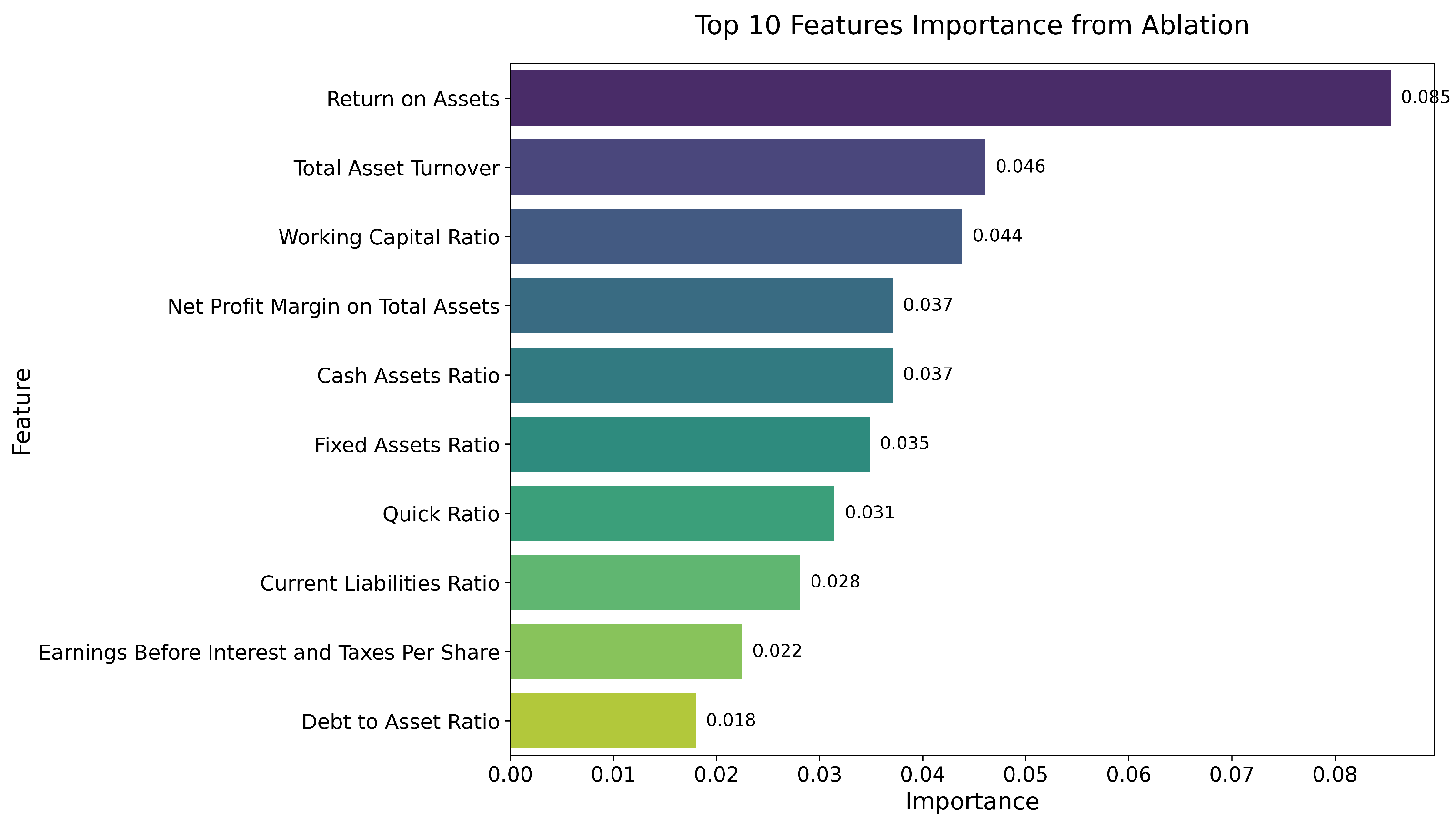
4.2. Sample and Indicator Selection

In this article, 890 Shanghai and Shenzhen A-share listed companies were selected from 2017 to 2024, and the sample data were from the Cathay Pacific CSMAR database. The specific experimental environment of this study was based on TensorFlow deep learning architecture, running on the Windows 10 operating system. Special treatment was implemented due to abnormal financial conditions (such as continuous losses in the past two years) as the sample data of ST companies, and companies that did not receive special treatment in the same year and are in the same industry with comparable asset sizes were selected as the sample data of non-ST companies. The year marked as ST is recorded as year T, and the previous year of ST is recorded as year T-1. In order to predict the financial difficulties in advance in the companies’ regular operation, we selected the quarterly financial index data from year T-3 to year T-5 as the sample characteristic data for prediction analysis. The financial data indicators are shown in

Table 1. Corporate financial data indicators.

Indicator Name	Description
Debt Service Capacity	Current ratio, quick ratio, cash ratio, working capital, debt-to-asset ratio, equity ratio, multiplier equity ratio
Ratio Structure	Current assets ratio, cash assets ratio, working capital ratio, non-current assets ratio, current liabilities ratio, fixed assets ratio, operating profit margin
Operating Capacity	Accounts receivable turnover, inventory turnover, accounts payable turnover, current asset turnover, fixed asset turnover, total asset turnover
Earnings Capacity	Return on assets, net profit margin on total assets, net profit margin on current assets, net profit margin on fixed assets, return on equity, operating profit rate
Cash Flow Capacity	Operating index
Development Capability	Capital preservation and appreciation rate, fixed asset growth rate, revenue growth rate, sustainable growth rate, owners’ equity growth rate
Per Share Metrics	Earnings per share, earnings before interest, taxes per share

. The sample distribution is shown in

Table 2. Sample distribution table.

Company Type	Number of Company Samples	Number of Time Series Data Points
ST	135	1620
Non-ST	755	9060
Total	890	10,680

Notes: Data sourced from the quarterly financial analysis module of the CSMAR database.

.

4.3. Data Preprocessing

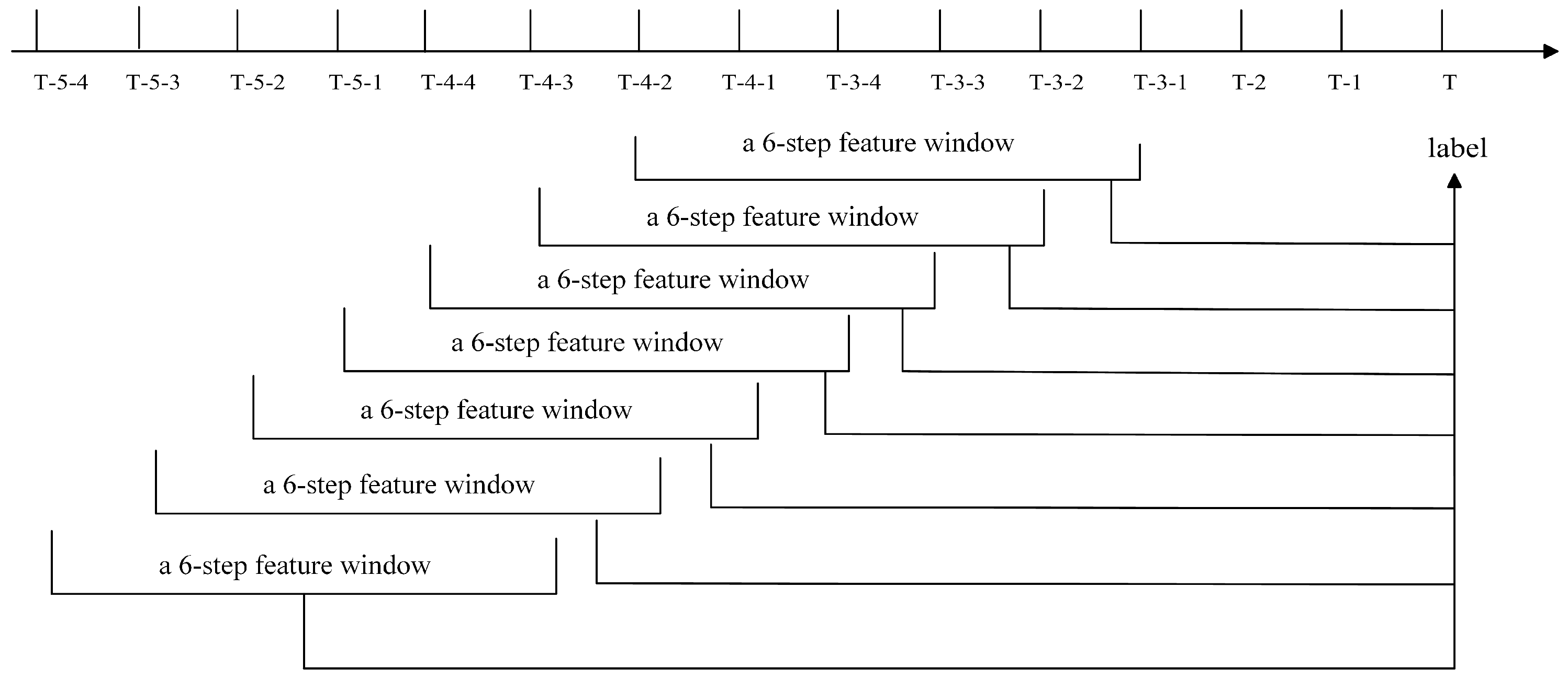
4.3.1. Sliding Window

A total of 135 ST and 755 non-ST companies were selected, with financial indicator data extracted for each company for 12 quarters over 3 years. This resulted in 1630 time series points for ST companies and 9060 for non-ST companies. The sliding window technique can generate feature windows and corresponding labels for subsequent analysis and model training. As shown in Figure 4, as an example of a sliding feature window of 6, windows are slid over the time series data to create overlapping windows. Each window contains six consecutive data points, and, for each feature window, a label was assigned from the subsequent time step, T, i.e., whether it was an ST company, which can effectively utilize the time series data to generate more training samples and improve the generalization ability of the model. Specifically, a six-step feature window was slid along each company’s financial time series with a stride of 1, creating overlapping input sequences. Each feature window consists of six consecutive quarters of financial data, and the corresponding label is determined by the ST status of the quarter immediately following the window (denoted as time T). The distribution of sliding window samples is shown in

Table 3. Distribution of sliding window samples.

Time Step	Training Data			Testing Data
	Non-ST	ST	Total	Non-ST	ST	Total
$w=4$	5346	972	6318	1359	243	1602
$w=5$	4832	864	5696	1208	216	1424
$w=6$	4228	756	4984	1057	189	1246
$w=7$	3624	648	4272	906	162	1068
$w=8$	3020	540	3560	772	118	890
$w=9$	2416	432	2848	604	108	712
$w=10$	1811	325	2136	454	80	534
$w=11$	1204	220	1424	306	50	356
$w=12$	603	109	712	152	26	178

Notes: ST denotes specially treated (financially distressed) companies, and non-ST denotes normal companies. Time step, w, refers to the sliding window length, i.e., the number of time points in each sample.

.

4.3.2. SMOTE Oversampling

The training set data were augmented using the synthetic minority over-sampling technique (SMOTE) method. SMOTE increases the number of minority samples by generating new synthetic samples around the minority class samples for data balancing. From

Table 4. Distribution of sliding window samples with oversampling.

Time Step	Original Training Data		Oversampled Training Data
	ST	Non-ST	ST	Non-ST
$w=4$	972	5346	5346	5346
$w=5$	864	4832	4832	4832
$w=6$	756	4228	4228	4228
$w=7$	648	3624	3624	3624
$w=8$	540	3020	3020	3020
$w=9$	432	2416	2416	2416
$w=10$	325	1811	1811	1811
$w=11$	220	1204	1204	1204
$w=12$	109	603	603	603

, taking time step 6 (w = 6) as an example, the number of samples of ST firms in the original training data was 756, and the number of samples of non-ST firms was 4228. Using the SMOTE method, new synthetic samples were generated to increase the number of samples of ST firms from 756 to 4228, which was equal to the number of samples of non-ST firms. SMOTE effectively increased the number of samples of the minority class (ST firms) and made the data more balanced and reduced the bias due to sample imbalance.

5. Results

5.1. Analysis of the Prediction Effect of Hyperband-CNN-BiLSTM-AT Model

5.1.1. Hyperband Algorithm Application

The number of neurons in the hidden layer of a neural network significantly impacts the model’s performance. Proper selection of the number of neurons in the hidden layer can help the model to fit the data better, while improper selection may lead to overfitting or underfitting. In order to verify the effectiveness of the Hyperband hyperparameter optimization method used, this study also selected two other common optimization strategies for comparison, namely random search and Bayesian optimization. All three methods perform a hyperparameter search under the same neural network structure, training epochs (epochs = 30), training and validation set partitioning strategy (validation_split = 0.2), and early stopping mechanism (EarlyStop) to ensure fairness in comparison. We recorded each method’s tuning time and final accuracy on the test set. The search space for the three-parameter tuning methods covers key parameters such as convolutional layer channels, LSTM layer units, dropout rate, and the number of fully connected layer neurons.

The optimal model for each method was evaluated on the test set, and their accuracy and time consumption are shown in

Table 5. Comparison of hyperparameter optimization methods.

Method	Time (Seconds)	Test Accuracy
Hyperband	2186.32	0.9876
Random search	628.25	0.9798
Bayesian optimization	591.74	0.9764

. The results show that, although Hyperband took the longest time, it achieves the highest model accuracy (0.9876). This indicates that its efficiency advantage in resource allocation can be explored more fully in a high-performance model configuration. Random search and Bayesian optimization have shorter testing times. However, their testing accuracy is slightly lower, indicating that Hyperband is more effective in discovering superior hyperparameter combinations under the constraint of a given number of experiments.

In this study, we mainly used the Hyperband algorithm to help select the appropriate number of neurons and other hyperparameter configurations. We first conducted preliminary experiments on Hyperband, random search, and Bayesian optimization within a small hyperparameter search space to determine appropriate parameter boundary intervals. On this basis, we further expanded the search scope and used the Hyperband method for a more comprehensive search to explore potential high-performance configurations fully. The range of hyperparameter search spaces and optimal configurations set are shown in

Table 6. Hyperparameter optimization results.

Hyperparameter	Search Scope	Step	Optimal Value
Conv_filters	[16, 128]	16	64
CNN_Dropout	[0.1, 0.5]	0.1	0.5
Bilstm_units1	[32, 128]	32	64
Bilstm_Dropout1	[0.1, 0.5]	0.1	0.2
Bilstm_units2	[32, 128]	32	128
Bilstm_Dropout2	[0.1, 0.5]	0.1	0.1
Dense_units1	[32, 256]	32	128
Dense_Dropout1	[0.1, 0.5]	0.1	0.1
Dense_units2	[32, 256]	32	128
Dense_Dropout2	[0.1, 0.5]	0.1	0.3

, where the Hyperband algorithm is set with the number of training rounds = 50, bandwidth factor = 3, and sub-stage i = 2, and the optimization objective is the accuracy of the test set. The search was run on the training set using 20% of the data for validation, with early stopping based on validation loss to prevent overfitting.

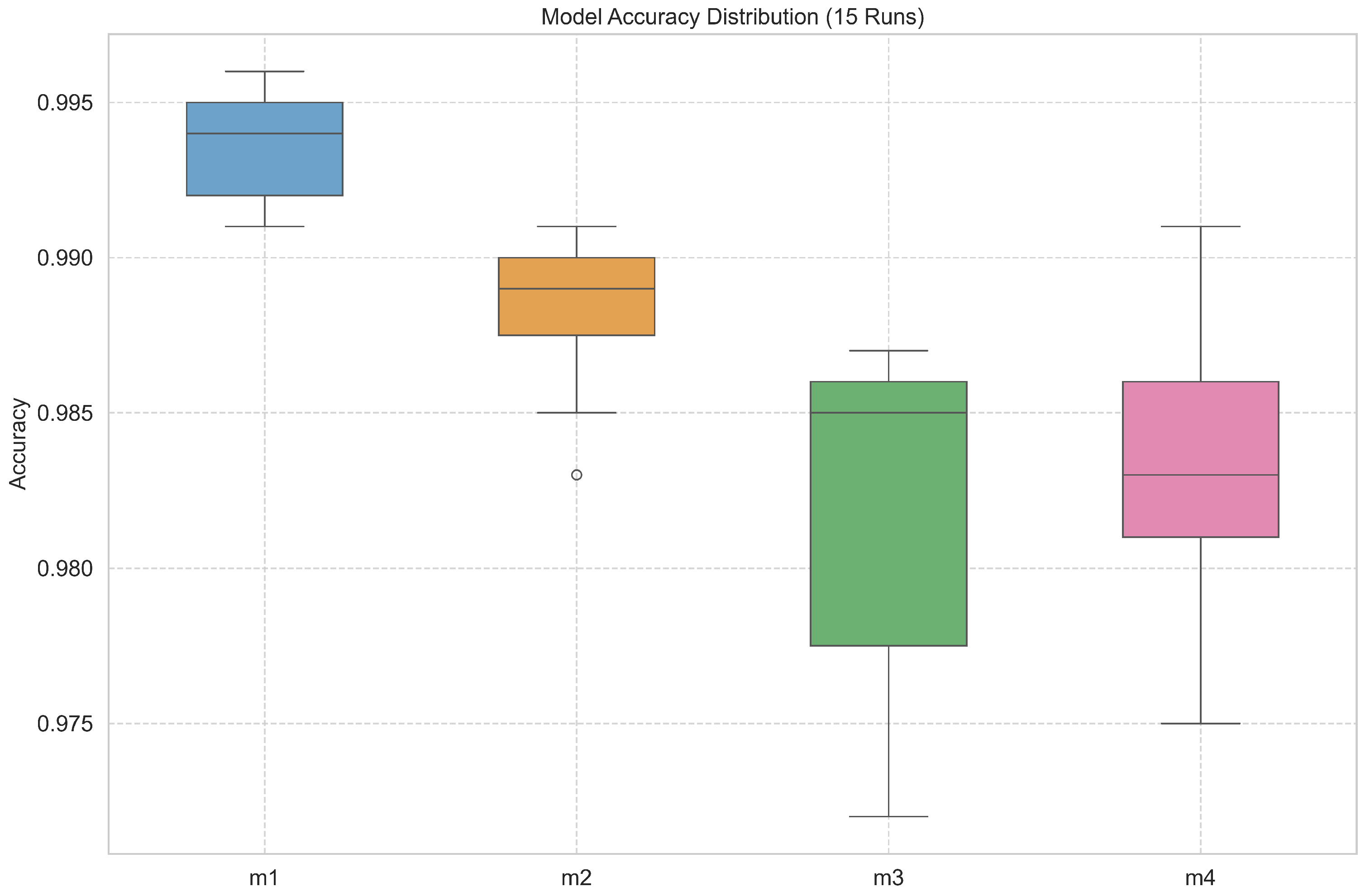
5.1.2. Comparative Analysis of CNN-BiLSTM-AT Model Structure

A series of experiments was designed to compare the effects of different model structures, batch counts, and time steps. The same dataset was used for training and evaluation: m1 represents 1 CNN layer + 1 BiLSTM layer + 1 AT layer, m1 represents 1 CNN layer + 2 BiLSTM layers + 1 AT layer, m3 represents 2 CNN layers + 1 BiLSTM layer + 1 AT layer, and m4 represents 2 CNN layers + 2 BiLSTM layers + 1 AT layer, as shown in

Table 7. CNN-BiLSTM-AT model structure table.

Layer	m1: 1CNN-1BiLSTM-AT	m2: 1CNN-2BiLSTM-AT	m3: 2CNN-1BiLSTM-AT	m4: 2CNN-2BiLSTM-AT
Conv1D	3 × 64 (ReLU)	3 × 64 (ReLU)	3 × 64 (ReLU)	3 × 64 (ReLU)
MaxPool	2 × 2	2 × 2	2 × 2	2 × 2
Conv1D	-	-	3 × 128 (ReLU)	3 × 128 (ReLU)
MaxPool	-	-	2 × 2	2 × 2
BiLSTM	64 (Tanh)	64 (Tanh)	64 (Tanh)	64 (Tanh)
BiLSTM	-	128 (Tanh)	-	128 (Tanh)
Attention	✔	✔	✔	✔
Dense	128 (ReLU)	128 (ReLU)	128 (ReLU)	128 (ReLU)

.

(1) Analysis of Results from Different Model Structures

Table 8. Comparison of CNN-BiLSTM-AT Model Performance.

Time Step	Batch Size = 32				Batch Size = 64
	m1	m2	m3	m4	m1	m2	m3	m4
$w=4$	0.948	0.947	0.917	0.923	0.956	0.946	0.917	0.908
$w=5$	0.963	0.958	0.946	0.928	0.955	0.961	0.946	0.935
$w=6$	0.984	0.987	0.953	0.967	0.984	0.983	0.972	0.960
$w=7$	0.982	0.980	0.968	0.966	0.978	0.977	0.969	0.970
$w=8$	0.994	0.987	0.987	0.981	0.985	0.987	0.980	0.976
$w=9$	0.993	0.993	0.973	0.976	0.990	0.985	0.979	0.987
$w=10$	0.983	0.979	0.983	0.968	0.987	0.981	0.974	0.981
$w=11$	0.941	0.958	0.916	0.924	0.952	0.941	0.930	0.955
$w=12$	0.820	0.787	0.792	0.781	0.798	0.792	0.798	0.815

Notes: m1 = 1CNN-1BiLSTM-AT; m2 = 1CNN-2BiLSTM-AT; m3 = 2CNN-1BiLSTM-AT; m4 = 2CNN-2BiLSTM-AT. Batch size denotes the number of samples used in each training iteration.

shows the accuracy of four models (m1 to m4) under different time steps (w) and batch sizes (batch_2) settings. Overall, as the time step increased, the model’s accuracy generally showed a trend of first increasing and then decreasing, especially reaching a high level of accuracy in the range of w = 6 to w = 10. When the time step was w = 8 and the batch size was 32, the accuracy of the m1 model was the highest at 99.4%.

From the perspective of model structure, the m1 and m2 models generally exhibited high accuracy in all time steps and batch size settings, especially in larger time steps (w = 6 to w = 10), where their performance was remarkably stable and excellent, demonstrating good learning and generalization abilities, whereas m3 and m4 exhibited inevitable fluctuations at specific time steps, with slightly lower overall accuracy, which may indicate that the model structures of m3 and m4 had relatively weak processing power in financial indicator series data.

From the perspective of batch size, there was no significant difference in model performance between the two batch size settings in most cases. However, in certain cases (m4 model from w = 5 to w = 12), the accuracy of models with a batch size of 32 was generally slightly higher.

From the perspective of time steps, models with smaller time steps (w = 4 to w = 5) exhibited relatively lower accuracy. The models showed high accuracy with larger time steps (w = 6 to w = 10). However, their performance sharply declined at w = 12, indicating that excessively long time steps caused dataset bias and made it difficult for the models to learn effectively.

To ensure the reliability of the significance test results and verify that the observed differences in model accuracy are not due to random chance, we did not fix the random seed during model training. Instead, each model was independently run 15 times with different random initializations. Figure 5 shows the accuracy distribution of the four models (m1, m2, m3, m4) in 15 experiments. The accuracy of m1 and m4 is relatively stable, while m2 and m3 exhibit significant fluctuations.

The average performance across these runs was used to conduct the Friedman test [23], a non-parametric statistical test suitable for comparing multiple models across multiple datasets. From

Table 9. Friedman test results of model performance comparison.

Model	m1	m2	m3	m4
Mean Rank	1.0000	2.3000	3.3333	3.3667
Friedman statistic	34.3061
p-value	0.000

, the resulting Friedman statistic was 34.3061 with a p-value of 0.000, indicating statistically significant differences among the models.

To further determine which models had significant differences, we used Bonferroni–Dunn post hoc testing [24]. From

Table 10. Post hoc comparison using Bonferroni correction.

Comparison	Z-Score	Bonferroni-Corrected p-Value
m1 and m2	2.7577	0.0349
m1 and m3	4.9497	0.0000
m1 and m4	5.0205	0.0000
m2 and m3	2.1920	0.1703
m2 and m4	2.2627	0.1419
m3 and m4	0.0707	1.0000

Notes: m1 = 1CNN-1BiLSTM-AT; m2 = 1CNN-2BiLSTM-AT; m3 = 2CNN-1BiLSTM-AT; m4 = 2CNN-2BiLSTM-AT.

, the results show that model m1 performed significantly better than m2, m3, and m4, with Bonferroni corrected p-values of 0.0349, 0.0000, and 0.0000, respectively. However, the differences between m2, m3, and m4 were insignificant (p > 0.05). These findings confirm that the performance improvement of m1 is statistically significant, rather than due to random variations.

(2) Results analysis of the best CNN-BiLSTM-AT models

After conducting experiments on different CNN-BiLSTM-AT model structures, we found that the m1 model (1CNN-1BiLSTM-AT) achieved the highest validation accuracy (0.994) at a time step of 8, batch size of 32, and 180 epochs of training. The loss value and accuracy trend chart in Figure 6 show that the model exhibits good convergence and stability during the training and validation process. This indicates that the m1 model has strong generalization ability and excellent performance under the current optimal configuration of the Hyperband algorithm, making it an ideal model structure.

According to the performance evaluation table for the best CNN-BiLSTM-AT model (

Table 11. Performance evaluation table of the best CNN-BiLSTM-AT models.

Sampling Method	Type	Precision	Recall	F1-Score	Accuracy
SMOTE	Non-ST	0.995	0.998	0.997	0.994
	ST	0.991	0.966	0.979
Non-SMOTE	Non-ST	0.985	0.992	0.988	0.979
	ST	0.946	0.898	0.922

), the overall accuracy was 99.4%, indicating strong performance. Among all samples predicted as the non-ST class, 99.5% were correctly identified as non-ST, and 99.8% of all predicted non-ST samples were accurately classified. For the ST class, 99.1% of predicted ST samples were correctly identified, while 96.6% of actual ST samples were accurately predicted as ST. In addition, compared with the model without SMOTE, the model’s accuracy was only 97.9%, and all evaluation indicators were lower than those of the SMOTE model, indicating the effectiveness of the SMOTE method.

(3) Feature Analysis of the Best CNN-BiLSTM-AT Model

① Key Features Highlighted by the Attention Mechanism

To interpret how the 1CNN-1BiLSTM-AT model identifies financial risks, we extracted and visualized the attention weights learned by the model. Specifically, the attention scores assigned to each financial indicator were averaged across all samples and time steps to obtain a global importance score. These scores were visualized in a horizontal bar chart (see Figure 7), where the top 10 features are ranked by their average attention weights. The results show that the model places the highest attention on the current asset turnover, working capital ratio, current assets ratio, inventory turnover, operating profit margin, current liabilities ratio, net profit margin on fixed assets, earnings before interest and taxes per share, operating profit rate, and net profit margin on total assets.

② Features Identified Through Ablation Study

This article used the feature ablation method to evaluate which features significantly impact the performance of the CNN-BiLSTM-AT model. This method trains a benchmark model using all features, records its performance metrics, removes each feature one by one, retrains the model, and evaluates the changes in model performance. A significant decrease in performance indicates that the feature is important to the model and ultimately determines the ranking of the feature. Figure 8 shows that the top 10 features had a significant impact on model performance: return on assets, total asset turnover, working capital ratio, net profit margin on total assets, cash assets ratio, fixed assets ratio, quick ratio, current liabilities ratio, earnings before interest and taxes per share, and debt-to-asset ratio.

The analysis combines the results of the attention mechanism and the ablation study to understand better how the model identifies key financial indicators. Several indicators, such as the working capital ratio, current liabilities ratio, net profit margin on total assets, and earnings before interest and taxes per share, are important in both methods, suggesting they play a consistent and critical role in financial distress prediction.

5.1.3. Comparison of Results from Different Models

Figure 9 and Figure 10, along with

Table 12. Performance evaluation of different models.

Model	ST			Non-ST			Training Time (s)
	Precision	Recall	F1-Score	Precision	Recall	F1-Score
CNN	0.990	0.814	0.893	0.972	0.999	0.985	162.52
BiLSTM	0.957	0.932	0.944	0.990	0.994	0.992	1279.94
CNN-BiLSTM	0.982	0.941	0.961	0.991	0.997	0.994	798.16
CNN-AT	0.982	0.949	0.966	0.992	0.997	0.995	163.34
BiLSTM-AT	0.958	0.958	0.958	0.994	0.994	0.994	1064.18
CNN-GRU	0.964	0.898	0.939	0.985	0.995	0.990	418.58
Transformer	0.982	0.957	0.970	0.994	0.997	0.995	151.87
CNN-BiLSTM-AT	0.991	0.966	0.979	0.995	0.999	0.997	430.97

, show the accuracy comparison results of six different models (w = 8, batch_size = 32), namely CNN, BiLSTM, CNN-BiLSTM, CNN-AT, BiLSTM-AT, CNN-GRU, Transformer, and CNN-BiLSTM-AT. From the figure, it can be seen that the CNN-BiLSTM-AT model performed the best with an accuracy of 0.994.

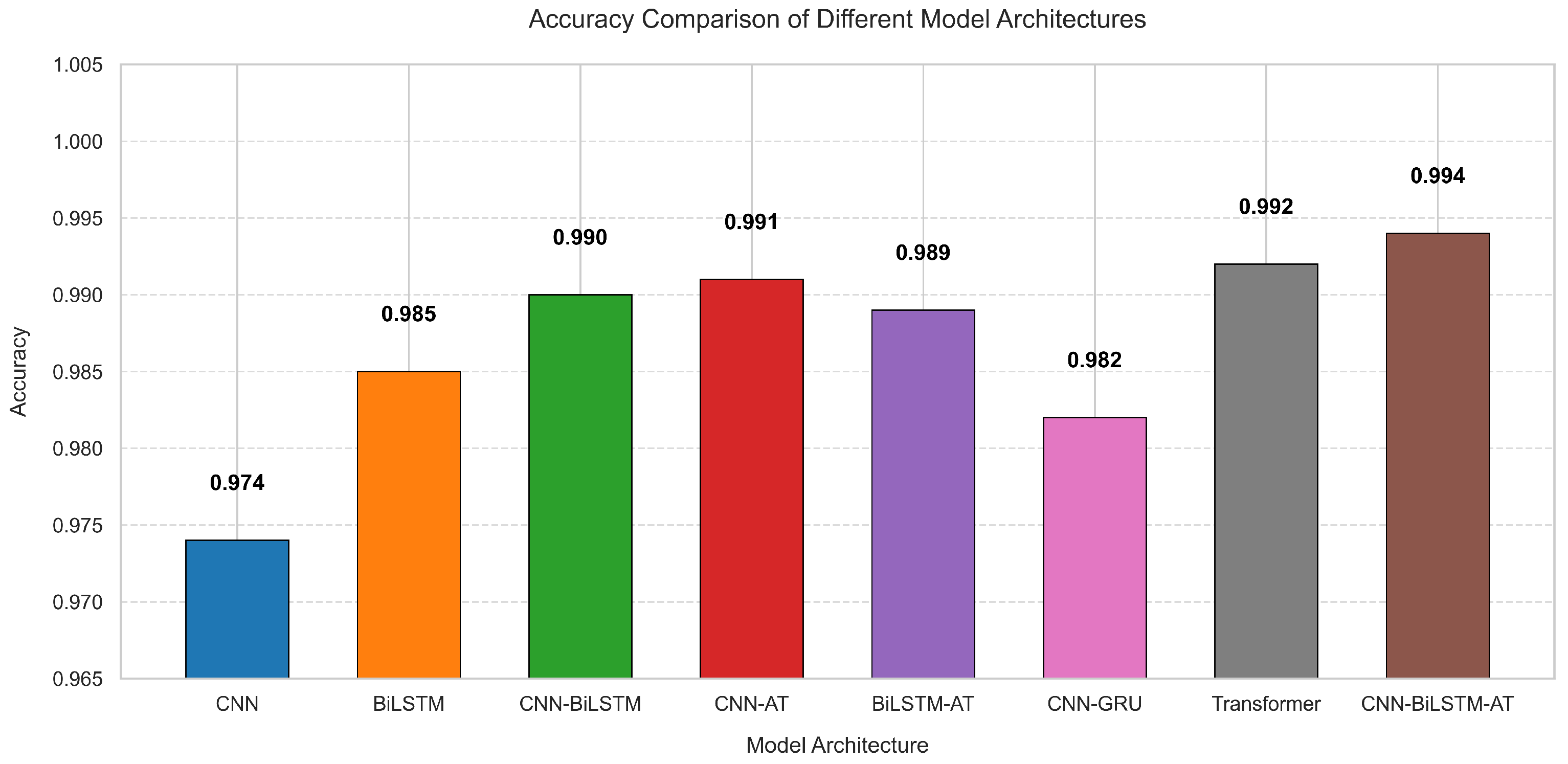
(1)

CNN model. The accuracy of this model was 0.974, showing it performed relatively well. However, it had the lowest accuracy among all models, mainly when predicting ST companies. Among the 118 actual ST sequence data points, 22 were mispredicted, and the recall rate was only 0.814. This indicates that using the CNN alone may not achieve optimal results when dealing with specific tasks. In addition, the model had a training time of 162.52 s, the shortest training time, and therefore is mainly suitable for use in scenarios with limited computing resources or requiring fast training.

(2)

BiLSTM model. The accuracy of this model was 0.985, which is significantly improved compared with the simple CNN model. The recall rate of ST samples was increased to 0.932, indicating that the model performs stably in identifying ST samples and performs better for time series data. In addition, the model took 1279.94 s to train, the longest training time. Although it performed well, the training time was relatively long, making it suitable for use in scenarios where resources are abundant or time is not tight.

(3)

CNN-BiLSTM model. This model’s accuracy was 0.990, performing better than CNN or BiLSTM. It also improved the accuracy and recall of predicting ST companies. In addition, the model’s training time was 798.16 s, which was shorter than the training time of the BiLSTM model alone. This indicates that the CNN can effectively extract features in the model, reduce the computational burden of BiLSTM, and thus accelerate the training speed.

(4)

CNN-AT model. The accuracy of this model was 0.991, which was better than using the CNN alone. The accuracy and recall of predicting ST companies were significantly improved, indicating that the combination of the CNN and attention mechanism gave a good performance in handling tasks that require attention to important features. Although the training time was 163.34 s, which was slightly longer than CNN, the performance improvement proved the effectiveness of this combination in enhancing the model’s predictive ability.

(5)

BiLSTM-AT model. This model’s accuracy was 0.989, outperforming BiLSTM used alone. It combines the advantages of BiLSTM and the attention mechanism and performs well in tasks that require long-term dependencies and important feature attention. In addition, the model’s training time was 1064.18 s. Although the performance improved, the training time was relatively long and unsuitable for fast iteration scenarios.

(6)

CNN-GRU model. The accuracy of this model was 0.982, which is an improvement compared with the standalone CNN model, but still lower than more complex structures such as CNN-BiLSTM and CNN-AT. Among 118 actual ST samples, the model had 12 prediction errors and a recall rate of 0.898, indicating that it still has some shortcomings in identifying ST companies. The training time was 418.58 s, which is at a moderate level.

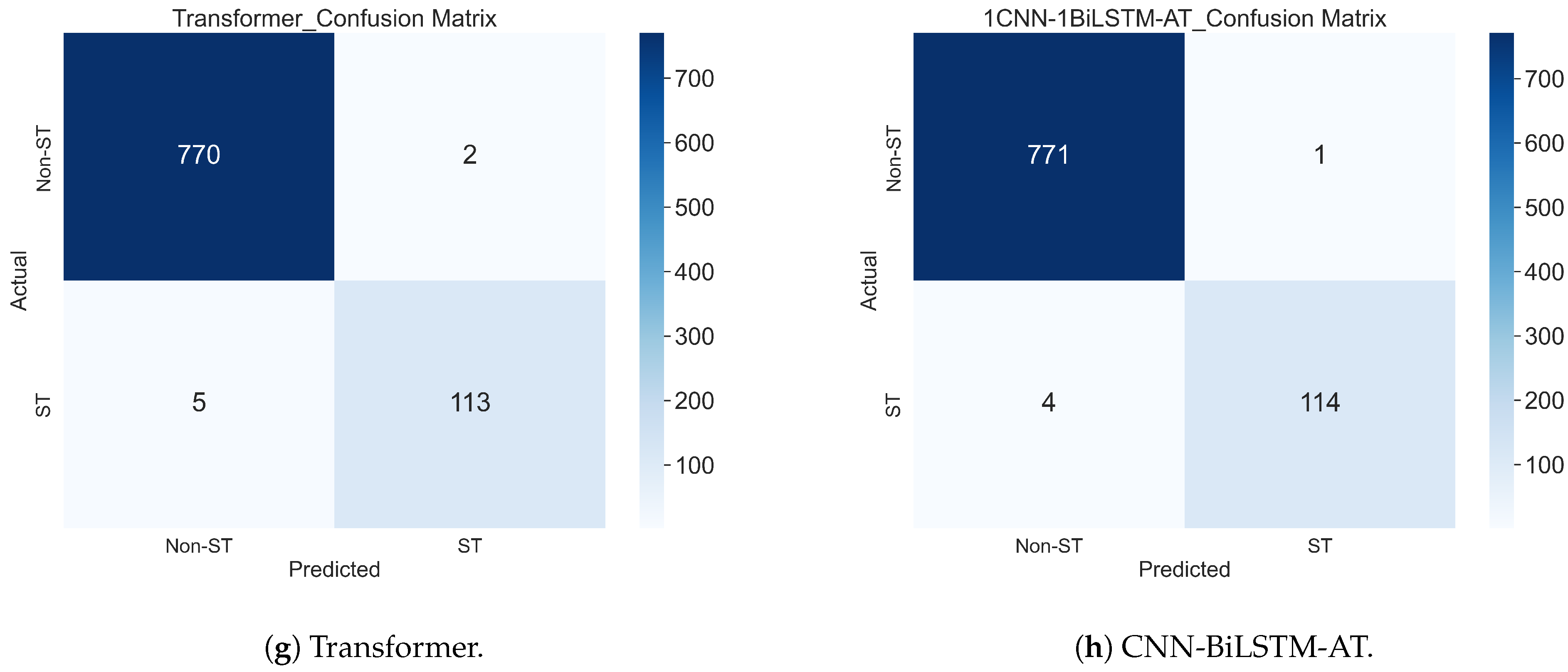
(7)

Transformer model. The accuracy of this model was 0.992, ranking high among all models, second only to the CNN-BiLSTM-AT model. This model utilized a self-attention mechanism to model the relationships between time points in the sequence, effectively capturing the global dependency features of the data and improving overall prediction performance. However, when predicting ST samples, its performance was slightly inferior to CNN-BiLSTM-AT, indicating that sensitivity to small sample categories still needs to be strengthened. The training time was 151.87 s, one of the shortest among all models.

(8)

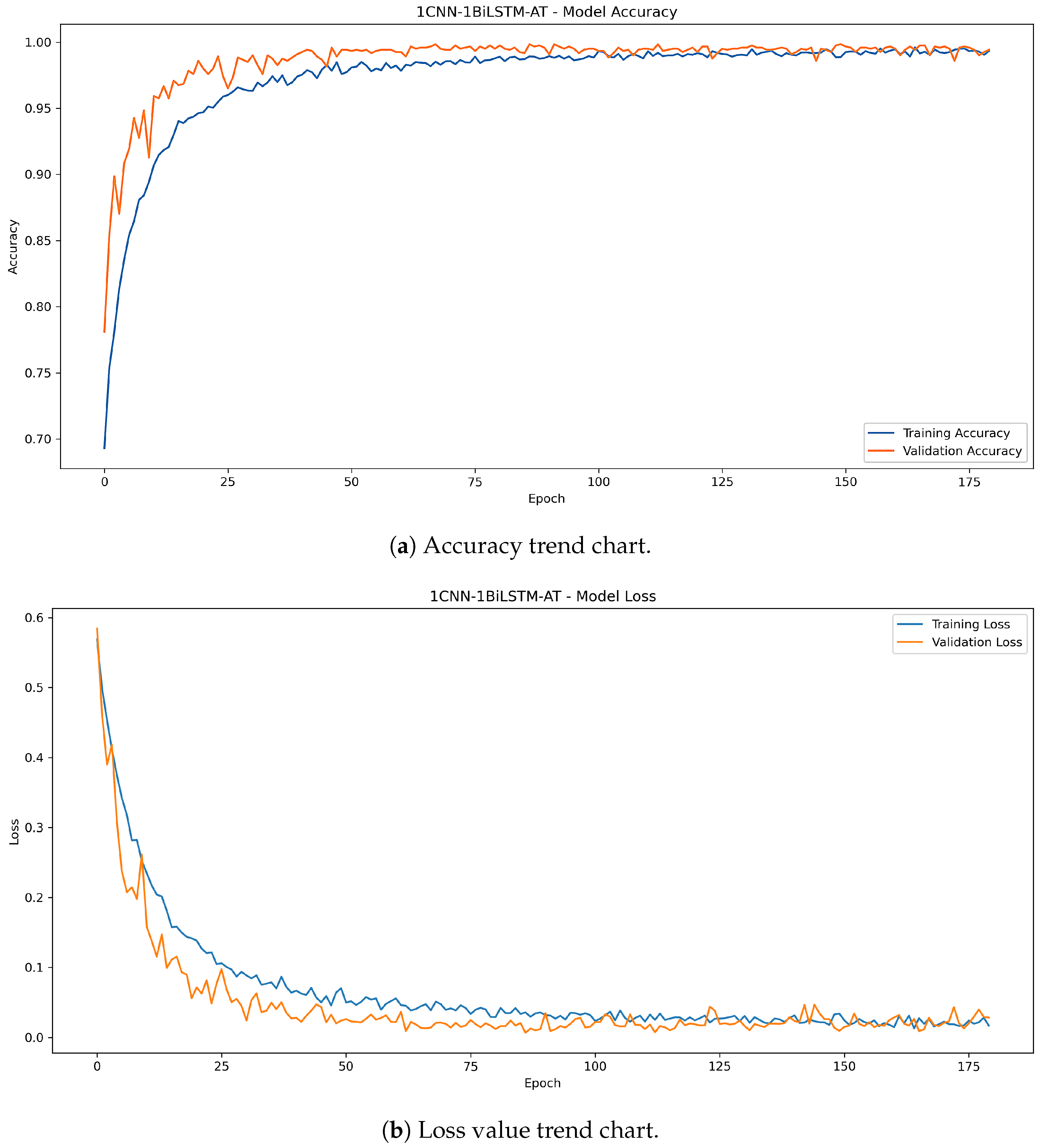
CNN-BiLSTM-AT model. The accuracy of this model was 0.994, and only five time data points were mispredicted. This indicates that this comprehensive model can fully utilize the features extracted by the convolutional layer, the time series information processed by BiLSTM, and the important features focused on by the attention mechanism to achieve the best results. Although the training time was 430.97 s, slightly longer than the CNN and CNN-AT models, its training time was still relatively short compared with the other models, and its overall performance was the best, making it an ideal choice for achieving a good balance between accuracy and efficiency.

5.2. Optimal Model Validation Analysis

To further validate the effectiveness and robustness of the constructed 1CNN-1BiLSTM-AT model, this article conducted in-depth testing of the model from two perspectives: firstly, evaluating the model’s performance outside the sample using new data from listed companies in 2025 to test its generalization ability on future data; and, secondly, selecting historical financial data of actual enterprises for case verification, in order to explore the applicability of the model in real business scenarios.

5.2.1. Data Validation in 2025

In the 2025 data validation, the financial data of listed companies in 2025 were used. The data were preprocessed and standardized, and time series features were constructed using sliding window technology. From

Table 13. Prediction classification report with 2025 data.

Class	Precision	Recall	F1-Score	Support
0	0.994	0.988	0.991	341
1	0.905	0.950	0.927	40
Macro Avg	0.949	0.969	0.959	381
Weighted Avg	0.985	0.984	0.984	381
Accuracy	0.984

, the verification results show that the 1CNN-1BiLSTM-AT model has good generalization ability, with an overall accuracy of 98.4%. Among them, the prediction accuracy and recall rate of category 0 (non-ST) are close to 99%; the accuracy of category 1 (ST) is 90.5%, the recall rate is 95.0%, and the F1 score is 92.7%. The overall performance is stable, indicating the model has good application prospects and predictive ability in practical scenarios.

5.2.2. Case Application Analysis

In order to achieve dynamic monitoring of financial distress of listed companies and verify the stability and effectiveness of the constructed model, this article selected the financial indicators of Company A and Company B in the past 12 quarters as inputs. It substituted them into the financial distress warning model based on CNN-BiLSTM-AT that had been built. One hundred repeated experiments with different random numbers of seeds were conducted. In each experiment, the model predicts the probability, p, of two companies facing financial distress, with a p-value range of [0, 1]. According to the judgment criteria set by the model, when the p-value is greater than 0.5, it is judged that the listed company is facing financial distress; when the p-value is less than or equal to 0.5, it is judged that the company is in a normal operating state.

Figure 11 and Figure 12 show the financial distress warning model results predicting the probability of financial distress faced by Company A and Company B under 100 different random numbers, respectively. Among them, for Company A, it was predicted that the minimum probability value of financial distress faced by the company in 100 repeated experiments was greater than 0.5, indicating that the company was facing financial distress. In 100 repeated experiments, using Company B, the probability of the company facing financial distress was predicted to be 0, which was less than 0.5, indicating that the company’s situation was normal. This indicates that the model can effectively distinguish whether a company is facing financial distress, further verifying the stability and reliability of the model in financial distress prediction, and meeting the actual financial distress prediction applications of listed companies.

6. Conclusions

6.1. Research Conclusions

This article proposes a CNN-BiLSTM-AT model optimized using the Hyperband algorithm, which predicts financial difficulties for listed companies based on their financial indicators over the past 3 years and 12 quarters. The empirical results demonstrated the model’s strong predictive performance across various configurations, notably achieving the highest accuracy of 0.994 with a time step of 8 and a batch size of 32. The complementary nature of the model’s structure enhances its ability to extract meaningful time series features. The CNN layers excel at capturing local patterns and short-term fluctuations, such as sudden changes in quarterly financial data, while the BiLSTM layers model long-term dependencies, helping the model grasp the trends and cycles of a company’s financial evolution. Additionally, the attention mechanism further strengthens the model’s ability to focus on critical financial indicators and key time points, allowing for more reasonable weight allocation.

The use of the SMOTE algorithm plays a crucial role in mitigating the bias caused by class imbalance, which is often a challenge in financial distress prediction, as financially troubled companies are relatively rare. Traditional models are often dominated by the majority class, which leads to the underrepresentation of minority class features. By generating synthetic samples, SMOTE improved the representation of distressed companies, allowing the model to learn their characteristics better, which significantly enhanced the recognition rate of financially distressed firms and, in turn, improved the overall predictive performance. The introduction of the Hyperband optimization algorithm further contributed to the model’s superior performance. Compared with random search and Bayesian optimization, Hyperband efficiently allocates resources to the most promising hyperparameter combinations, enabling the model to find better configurations in less time. Although Hyperband requires a slightly longer overall search time, its higher accuracy demonstrates its effectiveness in complex tasks with large parameter spaces. Feature ablation analysis combined with attention weights revealed that financial indicators such as the working capital ratio, return on assets, current ratio, and return on total assets consistently played significant roles in the model.

This model has important application value in financial decision-making and investment practice. Analyzing historical financial indicators and training them can lead to accurately predict financial difficulties, providing strong support for investors, credit analysts, and financial institutions. Key financial indicators such as return on assets, quick ratio, working capital ratio, current liabilities ratio, and net profit margin on total assets can help investors identify stable companies and avoid high-risk ones. Integrating this model into the early warning platform can enhance forward-looking and data-driven decision-making, reduce risks, and improve long-term returns, providing more accurate decision support for investors and financial institutions.

6.2. Research Limitations and Prospects

Although the model performs well in predicting financial distress, limitations remain. The model’s performance is highly dependent on the dataset used, and the current dataset only covers Chinese A-share listed companies. The research results may not directly apply to other markets or nonlisted companies, which limits their universality and applicability to some extent. In addition, although the model makes predictions based on historical financial data, it may not fully capture sudden market shocks, regulatory changes, or other external factors such as political events or global economic changes. The model did not consider textual data (such as news sentiment or social media indicators), which can provide valuable supplementary perspectives for predicting financial distress.

Another important limitation is that the model lacks sufficient transparency. Although the model can extract key financial indicators and the impact of these indicators has been identified, the internal decision-making process is still not straightforward enough due to the black box nature of deep learning methods. This lack of transparency is crucial for financial decision-making, as understanding the decision-making logic behind model predictions is key to improving decision trust and acceptability.

Future research can explore the adaptability of this model in different market environments, especially for nonlisted companies, to evaluate its robustness in different financial contexts. At the same time, combining external data sources such as macroeconomic indicators, market sentiment, and textual data may improve the accuracy of the model’s predictions of financial distress. In addition, it is crucial for future improvements to address the limitations of the model in handling complex, noisy, or unstructured data and enhancing its ability to respond to sudden market changes. Improving the transparency and interpretability of deep learning models will be a key research direction to promote their widespread acceptance in the financial field.

References

- Kuen, J.; Lim, K.M.; Lee, C.P. Self-taught learning of a deep invariant representation for visual tracking via temporal slowness principle. Pattern Recognit. 2015, 48, 2964–2982. [Google Scholar] [CrossRef]
- Gu, S.; Kelly, B.; Xiu, D. Empirical asset pricing via machine learning. Rev. Financ. Stud. 2020, 33, 2223–2273. [Google Scholar] [CrossRef]
- Hosaka, T. Bankruptcy prediction using imaged financial ratios and convolutional neural networks. Expert Syst. Appl. 2019, 117, 287–299. [Google Scholar] [CrossRef]
- Zhou, X.; Zhou, H.; Long, H. Forecasting the equity premium: Do deep neural network models work? Mod. Financ. 2023, 1, 1–11. [Google Scholar] [CrossRef]
- Li, S.; Chen, X. Research on Enterprise Financial Crisis Warning Model Based on Deep Learning Neural Network. Modern Inf. Technol. 2021, 5, 101–103+107. [Google Scholar]
- Aslam, S.; Rasool, A.; Jiang, Q.; Qu, Q. LSTM based model for real-time stock market prediction on unexpected incidents. In Proceedings of the 2021 IEEE International Conference on Real-Time Computing and Robotics (RCAR), Xining, China, 15–19 July 2021; pp. 1149–1153. [Google Scholar]
- Siami-Namini, S.; Tavakoli, N.; Namin, A.S. The performance of LSTM and BiLSTM in forecasting time series. In Proceedings of the 2019 IEEE International Conference on Big Data (Big Data), Los Angeles, CA, USA, 9–12 December 2019; pp. 3285–3292. [Google Scholar]
- Tao, L.H. Research on the Early Warning of Enterprise Financial Crisis Based on Transformer. Master’s Thesis, Hunan University of Science and Technology, Xiangtan, China, 2022. [Google Scholar]
- Ouyang, Z.S.; Lai, Y. Systemic financial risk early warning of financial market in China using Attention-LSTM model. N. Am. J. Econ. Financ. 2021, 56, 101383. [Google Scholar] [CrossRef]
- Zhao, Y. Design of a corporate financial crisis prediction model based on improved ABC-RNN+ Bi-LSTM algorithm in the context of sustainable development. PeerJ Comput. Sci. 2023, 9, e1287. [Google Scholar] [CrossRef]
- Chen, J.; Sun, B. Enhancing Financial Risk Prediction Using TG-LSTM Model: An Innovative Approach with Applications to Public Health Emergencies. J. Knowl. Econ. 2024, 16, 2979–2999. [Google Scholar] [CrossRef]
- Lu, W.; Li, J.; Wang, J.; Qin, L. A CNN-BiLSTM-AM method for stock price prediction. Neural Comput. Appl. 2021, 33, 4741–4753. [Google Scholar] [CrossRef]
- Kavianpour, P.; Kavianpour, M.; Jahani, E.; Ramezani, A. A CNN-BiLSTM model with attention mechanism for earthquake prediction. J. Supercomput. 2023, 79, 19194–19226. [Google Scholar] [CrossRef]
- Han, P.; Chen, H.; Rasool, A.; Jiang, Q.; Yang, M. MFB: A generalized multimodal fusion approach for bitcoin price prediction using time-lagged sentiment and indicator features. Expert Syst. Appl. 2025, 261, 125515. [Google Scholar] [CrossRef]
- Chen, J.; Liu, W. A study on stock price prediction based on Hyperband-LSTM model. Fin. Manag. Res. 2023, 1, 65–85. [Google Scholar]
- Fukushima, K. Neocognitron: A self-organizing neural network model for a mechanism of pattern recognition unaffected by shift in position. Biol. Cybern. 1980, 36, 193–202. [Google Scholar] [CrossRef]
- LeCun, Y.; Bottou, L.; Bengio, Y.; Haffner, P. Gradient-based learning applied to document recognition. Proc. IEEE 1998, 86, 2278–2324. [Google Scholar] [CrossRef]
- Gers, F.A.; Schmidhuber, J.; Cummins, F. Learning to forget: Continual prediction with LSTM. Neural Comput. 2000, 12, 2451–2471. [Google Scholar] [CrossRef]
- Hochreiter, S.; Schmidhuber, J. Long short-term memory. Neural Comput. 1997, 9, 1735–1780. [Google Scholar] [CrossRef]
- Bahdanau, D.; Cho, K.; Bengio, Y. Neural machine translation by jointly learning to align and translate. arXiv 2014, arXiv:1409.0473. [Google Scholar]
- Li, L.; Jamieson, K.; DeSalvo, G.; Rostamizadeh, A.; Talwalkar, A. Hyperband: A novel bandit-based approach to hyperparameter optimization. J. Mach. Learn. Res. 2018, 18, 1–52. [Google Scholar]
- Chawla, N.V.; Bowyer, K.W.; Hall, L.O.; Kegelmeyer, W.P. SMOTE: Synthetic minority over-sampling technique. J. Artif. Intell. Res. 2002, 16, 321–357. [Google Scholar] [CrossRef]
- Friedman, M. A comparison of alternative tests of significance for the problem of m rankings. Ann. Math. Stat. 1940, 11, 86–92. [Google Scholar] [CrossRef]
- Dunn, O.J. Multiple comparisons using rank sums. Technometrics 1964, 6, 241–252. [Google Scholar] [CrossRef]