Semi-Supervised Learning for Intrusion Detection in Large Computer Networks

Abstract

In an increasingly interconnected world, securing large networks against cyber-threats has become paramount as cyberattacks become more rampant, difficult, and expensive to remedy. This research explores data-driven security by applying semi-supervised machine learning techniques for intrusion detection in large-scale network environments. Novel methods (including decision tree with entropy-based uncertainty sampling, logistic regression with self-training, and co-training with random forest) are proposed to perform intrusion detection with limited labeled data. These methods leverage both available labeled data and abundant unlabeled data. Extensive experiments on the CIC-DDoS2019 dataset show promising results; both the decision tree with entropy-based uncertainty sampling and the co-training with random forest models achieve 99% accuracy. Furthermore, the UNSW-NB15 dataset is introduced to conduct a comparative analysis between base models (random forest, decision tree, and logistic regression) when using only labeled data and the proposed models when using partially labeled data. The proposed methods demonstrate superior results when using 1%, 10%, and 50% labeled data, highlighting their effectiveness and potential for improving intrusion detection systems in scenarios with limited labeled data.

1. Introduction

In our interconnected and digitized world, the security of digital networks has evolved from a concern to a necessity. The uninterrupted exchange of information across these networks underpins the operations of businesses, governments, and individuals alike. However, this connectivity introduces vulnerabilities that cyber attackers can exploit to compromise data integrity, confidentiality, and availability. Network intrusion in the form of unauthorized access to or manipulation of network resources remains a persistent threat, jeopardizing the trust upon which modern communication systems are built. The rapid evolution of technology has led to an increase in the complexity and scale of digital networks. As organizations migrate their operations to the cloud, adopt Internet of Things (IoT) devices, and process larger volumes of data, the attack surface for potential threats expands exponentially. The consequences of successful network breaches are far-reaching, encompassing financial loss, reputational damage, and even risks to public safety. High-profile breaches of financial institutions, government agencies, and multinational corporations underscore the urgency of safeguarding network infrastructure against malicious activities. As traditional methods of intrusion detection struggle to keep pace [1], there is a critical need for innovative solutions that can effectively address these evolving threats. The present study aims to fill this gap by investigating the application of semi-supervised machine learning techniques for intrusion detection in large network environments.

The primary aim of this work is to evaluate the effectiveness of these methods through extensive experimentation on large, complex, diverse, and imbalanced datasets such as CIC-DDoS2019 and UNSW-NB15. The secondary aim is to compare the proposed models with traditional fully-supervised models. By comparing the performance of the proposed semi-supervised models with that of traditional fully-supervised models, this research seeks to demonstrate the advantages of semi-supervised learning for intrusion detection. The principal conclusions highlight the potential for these methods to achieve high accuracy even with limited labeled data, offering a promising direction for future research and practical applications in cybersecurity.

2. Related Works

The current state of research highlights various approaches to intrusion detection, primarily relying on fully supervised machine learning models that require extensive labeled datasets. Examples of decision tree for intrusion detection in current research can be seen in [2,3,4]. Many papers have used K-nearest neighbor for intrusion detection [5,6,7]. Several other algorithms, including random forest [8,9,10] and neural networks [11,12,13], have also seen have notable research in the intrusion detection area. While the aforementioned research demonstrates the effectiveness of machine learning for intrusion detection, these approaches are not without limitations. Obtaining labeled data is often challenging and costly, leading to a growing interest in semi-supervised learning methods. Although key publications in the field have explored various semi-supervised techniques, there remains a need for comprehensive comparative studies that evaluate their effectiveness in real-world scenarios. Thus, there exists a continued need to strengthen computer systems and enhance their resilience against evolving cyber threats [14].

A variety of hypotheses exist regarding the optimal approach for semi-supervised intrusion detection, as seen in [15,16,17,18,19,20,21]. Some researchers advocate for more complex ensemble methods [22,23,24], while others emphasize the efficiency of simpler models combined with effective sampling techniques [25]. To address these debates and provide a clearer understanding of the potential benefits of semi-supervised learning in this context, this study proposes a number of novel methods, including decision tree with entropy-based uncertainty sampling, logistic regression with self-training, and co-training with random forest.

3. Methodology

This section provides a detailed description of the experimental setup, including the dataset, hardware, software, parameter settings, and methods used in this study, helping to ensure the results can be replicated and built upon.

3.1. Data Collection and Preprocessing

3.1.1. Description of the Dataset

The CIC-DDoS2019 dataset [26] is a substantial and diverse collection of network traffic data that closely resembles real-world network environments. It contains a wide range of network activities, including both normal and anomalous behavior, making it an ideal foundation for our intrusion detection research. The dataset has the following key characteristics:

• Size and Scope: The CIC-DDoS2019 dataset is substantial in size, containing a 30 gigabyte collection of network traffic records. It spans a wide range of network activities, making it suitable for both research and real-world application.
• Variety of Network Traffic: It comprises diverse network traffic data, encompassing legitimate network transactions and various forms of network attacks. The dataset includes BENIGN, DNS, LDAP, MSSQL, NetBIOS, NTP, SNMP, SSDP, UDP, Portmap, Syn, TFTP, and UDPLag data labels. This diversity reflects the complexity of real-world network environments.
• Real-World Relevance: The dataset is curated to mirror real-world scenarios, capturing network behaviors observed in operational networks. This real-world relevance ensures that the research findings are applicable to practical network security situations.
• Network Protocols: It covers a wide range of network protocols, including HTTP, TCP, UDP, ICMP, and others. This protocol diversity reflects the complexity of modern network communications.
• Traffic Features: Each network traffic record is associated with a set of features, which include flow characteristics, packet attributes, and temporal information. In total, the standard dataset before preprocessing contains 85 features. These features are essential for building effective intrusion detection models.
• Imbalanced Data: To mirror common real-world intrusion detection scenarios, the dataset exhibits class imbalance in which normal traffic significantly outweighs malicious traffic. Addressing class imbalance is a crucial aspect of our research.

The UNSW-NB15 dataset [27] is a widely recognized benchmark dataset for network intrusion detection that is designed to simulate real-world network environments and cyberattack scenarios. It serves as an excellent resource for evaluating intrusion detection models, and has been used extensively in research due to its comprehensive coverage of various attack types. The dataset has the following key characteristics:

• Size and Scope: The UNSW-NB15 dataset contains over 2.5 million network traffic records. The dataset’s large size ensures that it encompasses a broad spectrum of network behaviors, providing ample data for training and testing intrusion detection models.
• Variety of Network Traffic: The dataset includes a mix of legitimate (normal) network traffic and a wide range of attack vectors. In addition to normal traffic, it contains nine categories of attack labels: Fuzzers, Analysis, Backdoor, DoS, Exploits, Generic, Reconnaissance, Shellcode, and Worms. This variety offers a diverse set of data to evaluate the effectiveness of different detection techniques.
• Real-World Relevance: UNSW-NB15 was designed to replicate realistic network environments and modern-day cyber threats. It reflects the behavior of real-world traffic, making it highly relevant for evaluating security models aimed at practical deployment in current network security systems.
• Network Protocols: The dataset captures network flows that involve various protocols such as TCP, UDP, ICMP, and HTTP. The inclusion of multiple protocols makes it possible to explore a wide range of attack surfaces and defense mechanisms.
• Traffic Features: Each record in the UNSW-NB15 dataset includes 49 features, which cover both network flow characteristics and packet-level details. These features are critical for building robust machine learning models for intrusion detection. Key features include flow duration, service type, packet size, and content-based attributes.
• Imbalanced Data: As with many real-world intrusion detection datasets, UNSW-NB15 exhibits class imbalance, where the number of normal records is significantly larger than the attack records. This imbalance presents a challenge for machine learning models and underscores the need for specialized techniques to handle skewed data distributions.

3.1.2. Data Preprocessing

Data preprocessing plays a pivotal role in ensuring the quality and reliability of the CIC-DDoS2019 dataset for our intrusion detection research. In this section, we present the preprocessing pipeline along with the steps taken to clean and transform the raw data by addressing challenges such as duplicates, missing values, and outliers.

The preprocessing pipeline is as follows:

• Data cleaning and Transforming

  (i)

  Redundant data removal

  (ii)

  Imputation of missing values

  (iii)

  Imputation of infinite values

  (iv)

  Data type conversion

  (v)

  Managing inconsistencies in the data

• Feature Selection and Engineering

  (i)

  Label encoding

  (ii)

  Feature hashing

  (iii)

  Feature extraction

  (iv)

  Adding/removing features

These preprocessing steps collectively form the cornerstone of our methodology, ensuring that the CIC-DDoS2019 dataset is refined and ready for advanced analyses and model development. The decisions made during preprocessing align with the overarching goals of our research, emphasizing data quality, privacy preservation, and feature engineering to support effective intrusion detection models.

3.2. Design and Implementation

In the implementation of the intrusion detection system, we utilized various machine learning models to effectively classify network traffic. The implementation consists of three unique types of semi-supervised learning models

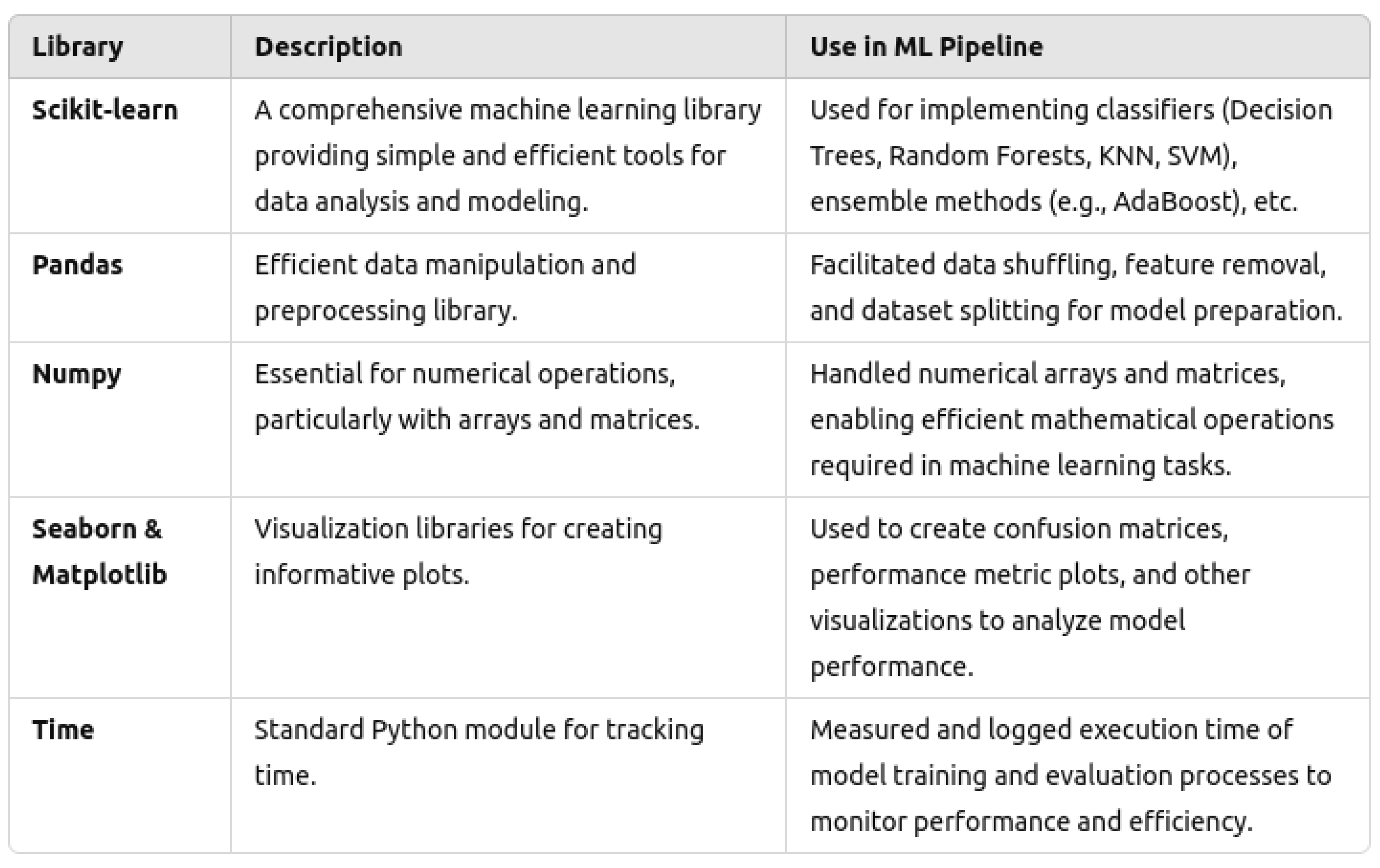
3.2.1. Libraries and Frameworks

The implementation leveraged popular Python 3.12 libraries and frameworks for machine learning, shown in Figure 1 below.

3.2.2. Hyperparameter Tuning Strategies

GridSearch was employed as the primary hyperparameter tuning strategy. Specifically, GridSearchCV from Scikit-learn was utilized to systematically search through a predefined hyperparameter space and identify the optimal configuration for each classifier. This iterative approach helped to fine-tune the models, maximizing their performance.

3.3. Proposed Semi-Supervised Learning Models

(1) Decision Tree with Entropy-based Uncertainty Sampling. Our first proposed model combines decision tree with entropy-based uncertainty sampling for semi-supervised learning, integrating concepts from decision trees, active learning, and semi-supervised learning. This approach was selected for its computational efficiency and ability to adapt to new and unseen data through query mechanisms [28,29]. A comprehensive overview is provided below.

3.3.1. Decision Trees

A decision tree is a machine learning model used for classification and regression. It works by recursively splitting the data into subsets based on feature values in order to create branches, aiming for maximum class separation [30]. The tree structure includes the following:

• Root Node: The top node, representing the entire dataset.
• Internal Nodes: Nodes representing tests on features.
• Branches: Outcomes of the tests.
• Leaf Nodes: Terminal nodes that represent class labels or regression values.

3.3.2. Entropy

Entropy measures the uncertainty or impurity in a dataset. In decision trees, it is used to calculate information gain, guiding the choice of features for splitting:

$$H\left(D\right)=-\sum _{i=1}^{k}p\left(c_i\right){log}_{2}p\left(c_i\right)$$

where $p\left(c_i\right)$ is the proportion of instances in class $c_i$.

Uncertainty sampling is an active learning strategy in which the model selects the most uncertain instances for labeling. Entropy-based uncertainty sampling chooses instances with the highest entropy, indicating maximum uncertainty:

$$H\left(x\right)=-\sum _{i=1}^{k}p\left(y_i\right|x){log}_{2}p\left(y_i\right|x).$$

3.3.3. Semi-Supervised Learning

Semi-supervised learning utilizes both labeled and unlabeled data to improve model performance, especially when labeled data are scarce or expensive. The idea is to leverage the abundant unlabeled data to gain better generalization capability.

3.3.4. Combining These Concepts

In semi-supervised learning with decision trees and entropy-based uncertainty sampling, the workflow typically includes the following:

• Initial Training: Start with a small labeled dataset and train a decision tree.
• Uncertainty Estimation: Use the trained decision tree to predict class probabilities for the unlabeled instances and calculate their entropy.
• Instance Selection: Select the unlabeled instances with the highest entropy for labeling.
• Labeling: Query an oracle (e.g., a human annotator) to obtain the true labels for these selected instances.
• Model Update: Retrain the decision tree with the expanded labeled dataset, now including the newly labeled instances.
• Iteration: Repeat the process of uncertainty estimation, instance selection, labeling, and model updating until a stopping criterion is met (e.g., a certain number of iterations, achieving a performance threshold, or exhausting the labeling budget).

The workflow is summarized in the following Algorithm 1.

Algorithm 1 Semi-Supervised Learning Workflow Using Decision Tree

Require:   Labeled dataset $\mathcal{L}$, Unlabeled dataset $\mathcal{U}$, Oracle for labeling; Ensure:  Trained Decision Tree Model $\mathcal{M}$;    1: Initialize: Train initial decision tree $\mathcal{M}$ on labeled set $\mathcal{L}$;    2: while stopping criterion not met do    3:     for each instance $x\in \mathcal{U}$ do    4:         Predict class probabilities for x using $\mathcal{M}$;    5:         Calculate uncertainty (entropy) $H\left(x\right)$ based on the predicted probabilities;    6:    end for    7:    Select instances with the highest entropy from $\mathcal{U}$;    8:    Request labels for the selected high-entropy instances from the oracle;    9:    Add newly labeled instances to $\mathcal{L}$ and remove them from $\mathcal{U}$;  10:    Retrain the decision tree $\mathcal{M}$ using the updated labeled set $\mathcal{L}$;  11: end while

(2) Logistic Regression with Self-Training. This model uses a self-training classifier with logistic regression as the base estimator. By combining logistic regression with self-training for semi-supervised learning, it integrates concepts from both logistic regression and semi-supervised learning. This approach was chosen for its binary classification suitability as well as to explore performance improvement through self-training [31,32]. A comprehensive overview is provided below.

3.3.5. Logistic Regression

Logistic regression is a statistical model used for binary classification tasks. It models the probability that a given input point belongs to a certain class [33]. The model uses the logistic function to map the predicted values to probabilities:

$$P(y=1|X)=\sigma (w^{T}X+b)={\displaystyle \frac{1}{1+e^{-(w^{T}X+b)}}}$$

where $\sigma$ is the sigmoid function, w is the weight vector, X is the input feature vector, and b is the bias term. The parameters w and b are learned by maximizing the likelihood of the observed data.

3.3.6. Self-Training

Self-training is a type of semi-supervised learning method in which the model is trained iteratively while using its own predictions to label the unlabeled data. The general process involves the following steps:

• Train the model on the initial labeled dataset.
• Use the trained model to predict labels for the unlabeled data.
• Select the most confident predictions and add them to the labeled dataset.
• Retrain the model on the updated labeled dataset.
• Repeat the process until a stopping criterion is met.

3.3.7. Combining These Concepts

In semi-supervised learning with logistic regression and self-training, the workflow typically includes the following steps:

• Initial Training: Train the logistic regression model on a small labeled dataset.
• Prediction: Use the trained model to predict probabilities for the unlabeled instances.
• Confidence Selection: Select the instances with the highest confidence (i.e., the highest predicted probabilities) for which the model is most certain.
• Labeling: Assign the predicted labels to these selected instances.
• Model Update: Add the newly labeled instances to the labeled dataset.
• Retraining: Retrain the logistic regression model with the expanded labeled dataset.
• Iteration: Repeat the process of prediction, selection, labeling, and retraining until a stopping criterion is met (e.g., a certain number of iterations, achieving a performance threshold, or exhausting the labeling budget).

The workflow is summarized in the Algorithm 2.

Algorithm 2 Semi-Supervised Learning Workflow Using Logistic Regression

Require:   Labeled dataset $\mathcal{L}$, Unlabeled dataset $\mathcal{U}$; Ensure:  Trained Logistic Regression Model $\mathcal{M}$;    1: Initialize: Train initial logistic regression model $\mathcal{M}$ on labeled set $\mathcal{L}$;    2: while stopping criterion not met do    3:     for each instance $x\in \mathcal{U}$ do    4:         Predict the probability $P(y=1|x)$ for x using $\mathcal{M}$;    5:     end for    6:     Select instances from $\mathcal{U}$ with the highest confidence (i.e., probabilities close to 0 or 1);    7:     Assign predicted labels to these high-confidence instances;    8:     Add newly labeled instances to $\mathcal{L}$ and remove them from $\mathcal{U}$;    9:     Retrain the logistic regression model $\mathcal{M}$ using the updated labeled set $\mathcal{L}$;  10: end while

(3) Co-Training with a Random Forest Base Estimator. This approach uses a co-training model with a random forest estimator as the base. Co-training with a random forest base estimator integrates concepts from both co-training and ensemble learning, and is adopted here for its high accuracy, robustness to class imbalance, and reduced exposure to overfitting [34,35]. A comprehensive overview is provided below.

3.3.8. Random Forest

Random forest is an ensemble learning method used for classification and regression tasks. It works by constructing multiple decision trees during training, then outputting the mode of the classes (classification) or the mean prediction (regression) of the individual trees [36]. Key characteristics include the following:

• Ensemble Method: Combines the predictions of several decision trees to improve generalization and robustness.
• Bagging: Uses bootstrap aggregation to create diverse subsets of the training data for each tree.
• Feature Randomness: Introduces additional randomness by selecting a random subset of features for each split in the trees.

3.3.9. Co-Training

Co-training is a semi-supervised learning algorithm that leverages multiple views of the data to improve learning. The basic idea is to train two classifiers on different views of the data and let them teach each other by labeling the unlabeled data:

• Multiple Views: It is assumed that the features can be split into two disjoint sets (views) that are sufficient to make predictions independently.
• Initial Training: Two classifiers (one for each view) are trained using the initial labeled dataset.
• Labeling: Each classifier labels the unlabeled instances that it is most confident about.
• Teaching: The labeled instances from one classifier are added to the training set of the other classifier.
• Iteration: The process is repeated iteratively to improve both classifiers.

3.3.10. Combining These Concepts

In semi-supervised learning with co-training and a random forest base estimator, the workflow typically includes the following:

• Initial Training: Train two random forest classifiers on different views of a small labeled dataset.
• Prediction: Use each random forest classifier to predict labels for the unlabeled instances.
• Confidence Selection: Select the instances with the highest confidence from each classifier’s predictions.
• Teaching: Add the confidently labeled instances from one classifier to the training set of the other classifier.
• Model Update: Retrain each random forest classifier with its expanded training set.
• Iteration: Repeat the process of prediction, selection, teaching, and retraining until a stopping criterion is met (e.g., a certain number of iterations, achieving a performance threshold, or exhausting the labeling budget).

The workflow is summarized in the following Algorithm 3.

Algorithm 3 Co-Training Workflow Using Random Forests on Split Feature Views

Require:   Labeled dataset $\mathcal{L}$, Unlabeled dataset $\mathcal{U}$, Feature views $V_1$ and $V_2$; Ensure:  Trained Random Forest models RF1 and RF2;    1: Initialize: Split features into two disjoint views $V_1$ and $V_2$;    2: Train initial Random Forest models RF1 on view $V_1$ and RF2 on view $V_2$ using labeled set $\mathcal{L}$;    3: while stopping criterion not met do    4:     for each instance $x\in \mathcal{U}$ do    5:         RF1 predicts the label for x using view $V_1$;    6:         RF2 predicts the label for x using view $V_2$;    7:     end for    8:     Select instances from $\mathcal{U}$ with the highest confidence from RF1 and RF2;    9:     Add the confidently labeled instances from RF1 to the training set of RF2, and vice versa;  10:     Update the labeled datasets for RF1 and RF2 with newly labeled instances;  11:     Retrain RF1 using the updated labeled set from view $V_1$, and RF2 using the updated labeled set from view $V_2$; 12: end while Note: ∈ is the mathematical symbol for “element of”.

4. Experimental Results and Discussion

4.1. Experimental Setup

This section provides the detailed experimental setup, including the datasets, hardware and software, and corresponding parameter settings.

4.2. Hardware

The experimental setup for this study utilized an IBM Power 8 server, which provides a robust and high-performance computing environment. The server was equipped with the following specifications:

• CPU Cores: 32
• CPU Speed: 4.22 GHz
• Memory: 1 TB (1024 GB)

4.3. Software

The following software was used to complete the research documented in this proposal:

• Python 3.7.6
• PyCharm (python version 3.8.10)
• RStudio 2023.03.0+386
• BigQuery

4.4. Parameter Settings

The parameter settings listed in

Table 1. Parameter settings used in the experimental setup.

Parameter	Setting
Software	PyCharm (Python version 3.8.10)
Packages	pandas (1.5.3), numpy (1.24.2), sklearn (1.2.2), scipy (1.10.1), matplotlib.pyplot (3.7.1), seaborn (0.12.2)
Functions/Modules	shuffle, train_test_split, classification_report, confusion_matrix, entropy
Classifiers	DecisionTreeClassifier, LogisticRegression, RandomForestClassifier
Data Tools	BigQuery

are the specific settings of the software used in the experimental setup.

4.5. Dataset Preparation and Coding

In terms of dataset preparation, most of the data preparation was the same for all of the models. The commonalities were as follows:

• Data shuffling: The dataset was shuffled for every model.
• Data splitting: For each model and its variants, 80% of the data was used for training and 20% was used for testing.
• Data stratification: The dataset was stratified for every model, which ensures that all labels are present in both training and testing.
• Second data splitting: All data were divided into scenarios in which 1%, 5%, 10%, 50%, or 100% of the training data were unlabeled.
• Data Reports: Classification reports and a confusion matrix were documented for each model.

4.6. Hyperparameters

4.6.1. Decision Tree with Entropy-Based Uncertainty Sampling

The following hyperparameters and parameters were used in the implementation:

• Data shuffling and splitting were performed with random_state = 42 to ensure reproducibility.
• For semi-supervised learning, entropy-based sampling was performed to select the most uncertain samples from the unlabeled data. n_samples = 20 were selected in each iteration.
• The semi-supervised learning process was iterated n_iterations = 10 times.

4.6.2. Logistic Regression with Self-Training

The following hyperparameters and parameters were used in the implementation:

• Data shuffling and splitting were performed with random_state = 42 to ensure reproducibility.
• A confidence threshold of 0.8 was used to add pseudo-labeled data to the labeled set.
• The self-training process was iterated max_iterations = 10 times.
• Class weights were assigned based on the presence of labels in the initially labeled data. Labels present in y_labeled were assigned a weight of 1.0, while others were assigned a weight of 0.5.

4.6.3. Co-Training with Random Forest

The following hyperparameters and parameters were used in the implementation:

• Data shuffling and splitting were performed with random_state = 42 to ensure reproducibility.
• The dataset was split into num_views = 2 different views, each using a subset of the features.
• Features were evenly split between the views, with

  features_per_view = len(X_train_labeled.columns) // num_views.

4.7. Results and Analysis

4.7.1. Evaluation Metrics

Evaluation metrics are numerical measures used to evaluate the performance and effectiveness of a statistical or machine learning model. These metrics offer insights into the model’s performance and facilitate the comparison of different models or algorithms.

4.7.2. Confusion Matrix

A confusion matrix is a vital tool when evaluating the performance of a classification algorithm. It is a table that is used to describe the performance of a classification model on a set of test data for which the true values are known. The matrix itself is easy to understand and provides a great deal of insight into the performance of the model. A confusion matrix for a binary classification problem is typically structured as follows:

	Predicted Positive	Predicted Negative
Actual Positive	True Positive (TP)	False Negative (FN)
Actual Negative	False Positive (FP)	True Negative (TN)

A breakdown of the terms is provided below:

True Positive (TP): The number of positive instances correctly predicted by the classifier.

False Negative (FN): The number of positive instances incorrectly predicted by the classifier as negative.

False Positive (FP): The number of negative instances incorrectly predicted by the classifier as positive.

True Negative (TN): The number of negative instances correctly predicted by the classifier.

Several performance metrics can be derived from the confusion matrix. These metrics are part of what is known as a classification report.

4.7.3. Classification Report

A classification report is a detailed performance evaluation of a classification algorithm. It provides key metrics for each class in a classification problem, helping to understand the performance of the model in more depth. The main metrics included in a classification report are precision, recall, F1-score, and support [37].

• Accuracy: The proportion of correctly classified instances (both true positives and true negatives) among the total instances:

  $$\mathrm{Accuracy}={\displaystyle \frac{TP+TN}{TP+TN+FP+FN}}.$$
• Precision: The proportion of true positive instances among those instances predicted as positive:

  $$\mathrm{Precision}={\displaystyle \frac{TP}{TP+FP}}.$$
• Recall (Sensitivity or True Positive Rate): The proportion of true positive instances among the actual positive instances:

  $$\mathrm{Recall}={\displaystyle \frac{TP}{TP+FN}}.$$
• Specificity (True Negative Rate): The proportion of true negative instances among the actual negative instances:

  $$\mathrm{Specificity}={\displaystyle \frac{TN}{TN+FP}}.$$
• F1-Score: The harmonic mean of precision and recall, which provides a balance between the two metrics:

  $$\mathrm{F}1-\mathrm{Score}=2·{\displaystyle \frac{\mathrm{Precision}·\mathrm{Recall}}{\mathrm{Precision}+\mathrm{Recall}}}.$$

In addition to per-class metrics, the classification report also provides the macro average and weighted average:

• Macro Average: Unweighted mean of the metrics for each class.
• Weighted Average: Mean of the metrics weighted by the support of each class.

The confusion matrix provides a comprehensive view of the performance of a classification model, allowing for the calculation of key metrics such as accuracy, precision, recall, specificity, and F1-score. These metrics help in understanding not only how many predictions were correct but also the types of errors made by the classifier. These insight are crucial for model evaluation and subsequent improvement.

In addition to providing a comprehensive overview of the performance of a classification model by detailing precision, recall, F1-score, and support for each class the classification report includes the macro and weighted averages, offering a balanced view of the model’s performance across all classes. This detailed analysis helps in understanding the strengths and weaknesses of the model and can guide further improvements.

4.7.4. Key Metrics

The metrics reported in this section are critical to assessing the performance of the proposed intrusion detection models under varying levels of labeled data. The accuracy metric quantifies how effectively the model distinguishes between normal and attack traffic, providing a direct measure of its classification performance. The misclassification metric highlights the number of samples from the large dataset that were incorrectly classified by the intrusion detection model. This metric is particularly useful for understanding the model’s limitations and its dependence on the amount of labeled data available during training. Followed by these is the classification report which provides a breakdown of the model performance by class.

4.7.5. Decision Tree with Entropy-Based Uncertainty Sampling

The performance of the decision tree model was evaluated with varying amounts of labeled data (1%, 5%, 10%, 50%, and 100%). A summary of the results is provided below.

4.7.6. Key Metrics

• Accuracy: Near-perfect across all levels of labeled data
• Misclassifications:

  –

  1% labeled data: 4225 samples

  –

  5% labeled data: 1408 samples

  –

  10% labeled data: 1408 samples

  –

  50% labeled data: 197 samples

  –

  100% labeled data: 98 samples

4.7.7. Performance by Class

The performance of the proposed method is given in

Table 2. Classification report (1% labeled data).

Class	Precision	Recall	F1-Score	Support
0.0	0.9787	0.9687	0.9737	22,766
1.0	0.9996	0.9995	0.9995	1,014,202
2.0	0.9997	0.9998	0.9998	819,011
3.0	0.9998	0.9998	0.9998	2,061,989
4.0	0.9995	0.9997	0.9996	1,550,155
5.0	0.9995	0.9994	0.9994	240,528
6.0	0.9996	0.9998	0.9997	1,031,974
7.0	0.9998	0.9996	0.9997	522,122
8.0	0.9998	0.9997	0.9997	1,400,360
9.0	0.9954	0.9984	0.9969	37,392
10.0	0.9997	0.9996	0.9996	1,294,758
11.0	1.0000	0.9999	1.0000	4,016,516
12.0	0.9954	0.9992	0.9973	73,667
13.0	0.7778	0.4773	0.5915	88
Accuracy	0.9997 (14,085,528)
Macro Avg	0.9817	0.9600	0.9683	14,085,528
Weighted Avg	0.9997	0.9997	0.9997	14,085,528

,

Table 3. Classification report (5% labeled data).

Class	Precision	Recall	F1-Score	Support
0.0	0.9931	0.9881	0.9906	22,766
1.0	0.9999	0.9999	0.9999	1,014,202
2.0	0.9999	0.9999	0.9999	819,011
3.0	1.0000	1.0000	1.0000	2,061,989
4.0	0.9999	0.9999	0.9999	1,550,155
5.0	0.9998	0.9998	0.9998	240,528
6.0	0.9999	1.0000	0.9999	1,031,974
7.0	0.9999	0.9998	0.9999	522,122
8.0	0.9999	0.9999	0.9999	1,400,360
9.0	0.9981	0.9996	0.9988	37,392
10.0	0.9999	1.0000	1.0000	1,294,758
11.0	1.0000	1.0000	1.0000	4,016,516
12.0	0.9996	0.9996	0.9996	73,667
13.0	0.9667	0.9886	0.9775	88
Accuracy	0.9999 (14,085,528)
Macro Avg	0.9969	0.9982	0.9975	14,085,528
Weighted Avg	0.9999	0.9999	0.9999	14,085,528

,

Table 4. Classification report (10% labeled data).

Class	Precision	Recall	F1-Score	Support
0.0	0.9957	0.9939	0.9948	22,766
1.0	0.9999	1.0000	1.0000	1,014,202
2.0	1.0000	1.0000	1.0000	819,011
3.0	1.0000	1.0000	1.0000	2,061,989
4.0	0.9999	1.0000	1.0000	1,550,155
5.0	0.9999	1.0000	1.0000	240,528
6.0	0.9999	1.0000	1.0000	1,031,974
7.0	1.0000	0.9999	1.0000	522,122
8.0	1.0000	1.0000	1.0000	1,400,360
9.0	0.9992	0.9994	0.9993	37,392
10.0	1.0000	1.0000	1.0000	1,294,758
11.0	1.0000	1.0000	1.0000	4,016,516
12.0	0.9994	0.9995	0.9994	73,667
13.0	0.9322	0.9659	0.9487	88
Accuracy	0.9999 (14,085,528)
Macro Avg	0.9975	0.9983	0.9979	14,085,528
Weighted Avg	0.9999	0.9999	0.9999	14,085,528

,

Table 5. Classification report (50% labeled data).

Class	Precision	Recall	F1-Score	Support
0.0	0.9987	0.9987	0.9987	22,766
1.0	1.0000	1.0000	1.0000	1,014,202
2.0	1.0000	1.0000	1.0000	819,011
3.0	1.0000	1.0000	1.0000	2,061,989
4.0	1.0000	1.0000	1.0000	1,550,155
5.0	1.0000	1.0000	1.0000	240,528
6.0	1.0000	1.0000	1.0000	1,031,974
7.0	1.0000	1.0000	1.0000	522,122
8.0	1.0000	1.0000	1.0000	14,00,360
9.0	0.9999	0.9999	0.9999	37,392
10.0	1.0000	1.0000	1.0000	1,294,758
11.0	1.0000	1.0000	1.0000	4,016,516
12.0	0.9999	0.9999	0.9999	73,667
13.0	0.9647	0.9886	0.9765	88
Accuracy	0.999999 (14,085,528)
Macro Avg	0.9987	0.9990	0.9988	14,085,528
Weighted Avg	1.0000	1.0000	1.0000	14,085,528

and

Table 6. Classification report (100% labeled data).

Class	Precision	Recall	F1-Score	Support
0.0	0.9993	0.9994	0.9993	22,766
1.0	1.0000	1.0000	1.0000	1,014,202
2.0	1.0000	1.0000	1.0000	819,011
3.0	1.0000	1.0000	1.0000	2,061,989
4.0	1.0000	1.0000	1.0000	1,550,155
5.0	1.0000	1.0000	1.0000	240,528
6.0	1.0000	1.0000	1.0000	1,031,974
7.0	1.0000	1.0000	1.0000	522,122
8.0	1.0000	1.0000	1.0000	1,400,360
9.0	0.9999	1.0000	0.9999	37,392
10.0	1.0000	1.0000	1.0000	1,294,758
11.0	1.0000	1.0000	1.0000	4,016,516
12.0	1.0000	1.0000	1.0000	73,667
13.0	0.9667	0.9886	0.9775	88
Accuracy	0.999999 (14,085,528)
Macro Avg	0.9987	0.9990	0.9988	14,085,528
Weighted Avg	1.0000	1.0000	1.0000	14,085,528

corresponding to $1\%$, $5\%$, $10\%$, $50\%$ and $100\%$ of the labeled data, respectively.

4.7.8. Highlights

Class 11 consistently exhibits the highest performance metrics across all levels of labeled data. With a substantial support of 4,016,516 samples, this class demonstrates near-perfect precision, recall, and F1-score. This consistently high performance suggests that the decision tree model is particularly adept at accurately classifying instances belonging to Class 11, indicating robust representation of its distinguishing features within the dataset.

Class 13 presents a contrasting scenario, with the lowest performance metrics among all classes. This poor performance is primarily attributed to its significantly smaller support of only 88 samples. With lower support, the model has less data to learn from, leading to difficulties in accurately capturing the intricate patterns and nuances specific to Class 13. As a result, precision, recall, and F1-score for this class are comparatively lower, indicating a higher rate of misclassifications or difficulties in identifying its instances correctly.

Compared to the macro average, the weighted average emphasizes the significance of considering class imbalances when evaluating the model’s overall performance. The weighted average takes into account the contribution of each class in proportion to its support, providing a more accurate representation of the model’s effectiveness across the entire dataset. In contrast, the macro average treats each class equally, potentially skewing the assessment toward classes with larger support. The consistently higher weighted average reflects this model’s strong performance across classes with substantial support, indicating robustness in handling imbalanced datasets and accurate classification of majority classes while maintaining competitive performance for smaller classes.

4.7.9. Logistic Regression with Self-Training

The performance of the logistic regression model was evaluated with varying amounts of labeled data (1%, 5%, 10%, 50%, and 100%). A summary of the results is provided below:

4.7.10. Key Metrics

• Accuracy: Suboptimal across all levels of labeled data
• Misclassifications:

  –

  1% labeled data: 9,654,220 samples

  –

  5% labeled data: 9,844,375 samples

  –

  10% labeled data: 9,809,161 samples

  –

  50% labeled data: 9,559,847 samples

  –

  100% labeled data: 8,875,291 samples

4.7.11. Performance by Class

The performance of the proposed method is given in

Table 7. Classification report (1% labeled data).

Class	Precision	Recall	F1-Score	Support
0.0	0.0000	0.0000	0.0000	22,766
1.0	0.2090	0.2500	0.2277	1,014,202
2.0	0.0000	0.0000	0.0000	819,011
3.0	0.2850	0.8989	0.4327	2,061,989
4.0	0.2012	0.4039	0.2686	1,550,155
5.0	0.0000	0.0000	0.0000	240,528
6.0	0.0000	0.0000	0.0000	1,031,974
7.0	0.0000	0.0000	0.0000	522,122
8.0	0.0000	0.0000	0.0000	1,400,360
9.0	0.0000	0.0000	0.0000	37,392
10.0	0.9326	0.2691	0.4177	1,294,758
11.0	0.4681	0.3360	0.3912	4,016,516
12.0	0.0000	0.0000	0.0000	73,667
13.0	0.0000	0.0000	0.0000	88
Accuracy	0.3146 (14,085,528)
Macro Avg	0.1497	0.1541	0.1241	14,085,528
Weighted Avg	0.2981	0.3146	0.2593	14,085,528

,

Table 8. Classification report (5% labeled data).

Class	Precision	Recall	F1-Score	Support
0.0	0.0000	0.0000	0.0000	22,766
1.0	0.2005	0.1208	0.1508	1,014,202
2.0	0.0000	0.0000	0.0000	819,011
3.0	0.2784	0.8963	0.4248	2,061,989
4.0	0.1716	0.4095	0.2419	1,550,155
5.0	0.0000	0.0000	0.0000	240,528
6.0	0.0000	0.0000	0.0000	1,031,974
7.0	0.0000	0.0000	0.0000	522,122
8.0	0.0000	0.0000	0.0000	1,400,360
9.0	0.0000	0.0000	0.0000	37,392
10.0	0.9349	0.2806	0.4317	1,294,758
11.0	0.4631	0.3167	0.3762	4,016,516
12.0	0.0000	0.0000	0.0000	73,667
13.0	0.0000	0.0000	0.0000	88
Accuracy	0.3011 (14,085,528)
Macro Avg	0.1463	0.1446	0.1161	14,085,528
Weighted Avg	0.2921	0.3011	0.2466	14,085,528

,

Table 9. Classification report (10% labeled data).

Class	Precision	Recall	F1-Score	Support
0.0	0.0000	0.0000	0.0000	22,766
1.0	0.2660	0.1160	0.1615	1,014,202
2.0	0.0000	0.0000	0.0000	819,011
3.0	0.2879	0.9578	0.4427	2,061,989
4.0	0.1327	0.2492	0.1732	1,550,155
5.0	0.0000	0.0000	0.0000	240,528
6.0	0.0000	0.0000	0.0000	1,031,974
7.0	0.0000	0.0000	0.0000	522,122
8.0	0.0000	0.0000	0.0000	1,400,360
9.0	0.0000	0.0000	0.0000	37,392
10.0	0.9291	0.2780	0.4231	1,294,758
11.0	0.4820	0.3184	0.3848	4,016,516
12.0	0.0000	0.0000	0.0000	73,667
13.0	0.0000	0.0000	0.0000	88
Accuracy	0.3082 (14,085,528)
Macro Avg	0.1507	0.1501	0.1205	14,085,528
Weighted Avg	0.2957	0.3082	0.2551	14,085,528

,

Table 10. Classification report (50% labeled data).

Class	Precision	Recall	F1-Score	Support
0.0	0.0000	0.0000	0.0000	22,766
1.0	0.2457	0.1364	0.1760	1,014,202
2.0	0.0000	0.0000	0.0000	819,011
3.0	0.2892	0.9569	0.4432	2,061,989
4.0	0.1698	0.3521	0.2305	1,550,155
5.0	0.0000	0.0000	0.0000	240,528
6.0	0.0000	0.0000	0.0000	1,031,974
7.0	0.0000	0.0000	0.0000	522,122
8.0	0.0000	0.0000	0.0000	1,400,360
9.0	0.0000	0.0000	0.0000	37,392
10.0	0.9324	0.2822	0.4324	1,294,758
11.0	0.4653	0.3072	0.3680	4,016,516
12.0	0.0000	0.0000	0.0000	73,667
13.0	0.0000	0.0000	0.0000	88
Accuracy	0.3042 (14,085,528)
Macro Avg	0.1502	0.1467	0.1165	14,085,528
Weighted Avg	0.2944	0.3042	0.2506	14,085,528

and

Table 11. Classification report (100% labeled data).

Class	Precision	Recall	F1-Score	Support
0.0	0.0000	0.0000	0.0000	22,766
1.0	0.2597	0.1431	0.1856	1,014,202
2.0	0.0000	0.0000	0.0000	819,011
3.0	0.2900	0.9554	0.4441	2,061,989
4.0	0.1664	0.3217	0.2206	1,550,155
5.0	0.0000	0.0000	0.0000	240,528
6.0	0.0000	0.0000	0.0000	1,031,974
7.0	0.0000	0.0000	0.0000	522,122
8.0	0.0000	0.0000	0.0000	1,400,360
9.0	0.0000	0.0000	0.0000	37,392
10.0	0.9346	0.2801	0.4312	1,294,758
11.0	0.4601	0.3011	0.3627	4,016,516
12.0	0.0000	0.0000	0.0000	73,667
13.0	0.0000	0.0000	0.0000	88
Accuracy	0.3007 (14,085,528)
Macro Avg	0.1500	0.1442	0.1158	14,085,528
Weighted Avg	0.2928	0.3007	0.2463	14,085,528

corresponding to $1\%$, $5\%$, $10\%$, $50\%$ and $100\%$ of the labeled data, respectively.

4.7.12. Highlights

Class 0 and Class 2 show very poor performance metrics (precision, recall, F1-score: 0.0000) across all levels of labeled data. These results indicate that the model struggles significantly with these classes, potentially due to inadequate feature representation or insufficient labeled data for these specific classes.

Class 3 shows strong recall across all levels of labeled data, particularly with 10% and higher. This high recall, reaching as high as 95.78% with 10% labeled data, indicates the model’s ability to correctly identify the majority of Class 3 instances. However, the precision for this class is moderate, suggesting that while most Class 3 instances are identified, there are still a significant number of false positives.

Class 10 has high precision (around 93%) but relatively low recall (around 28%) across all labeled data levels. This indicates that while the model is very accurate when it predicts Class 10, it misses a significant number of instances, leading to a moderate F1-score.

Class 11 consistently exhibits relatively high performance metrics across all levels of labeled data. With substantial support of 4,016,516 samples, this class shows consistent precision, recall, and F1-score. Although not perfect, the consistent performance suggests that the logistic regression model is particularly adept at classifying instances belonging to Class 11, indicating robust representation of its distinguishing features within the dataset.

Class 13 presents a contrasting scenario, with the lowest performance metrics among all classes. This poor performance is primarily attributed to its significantly smaller support of only 88 samples. With lower support, the model has less data to learn from, leading to difficulties in accurately capturing the intricate patterns and nuances specific to Class 13. As a result, precision, recall, and F1-score for this class are 0.0000, indicating a higher rate of misclassifications or difficulties in correctly identifying its instances.

Compared to the macro averages, the weighted averages emphasize the significance of considering class imbalance when evaluating the model’s overall performance. The weighted average takes into account the contribution of each class in proportion to its support, providing a more accurate representation of the model’s effectiveness across the entire dataset. In contrast, the macro average treats each class equally, potentially skewing the assessment towards classes with larger supports. The consistently higher weighted averages reflect this model’s stronger performance across classes with substantial support, indicating its robustness when handling imbalanced datasets and ability to accurately classify majority classes while maintaining competitive performance in smaller classes.

Class imbalance significantly affects model performance, as can be seen in the classes with high and low support. Classes with higher support generally perform better due to more data being available for the model to learn from. Conversely, classes with lower support struggle with poor performance metrics, highlighting challenges in capturing the nuanced patterns of less frequent classes.

4.7.13. Co-Training with Random Forest Base Estimator

The performance of the co-training model with a random forest base estimator was evaluated with varying amounts of labeled data (1%, 5%, 10%, 50%, and 100%). A summary of the results is provided below:

4.7.14. Key Metrics

• Accuracy: Very high across all levels of labeled data
• Misclassifications:

  –

  1% labeled data: 140,869 samples

  –

  5% labeled data: 140,855 samples

  –

  10% labeled data: 140,855 samples

  –

  50% labeled data: 140,855 samples

  –

  100% labeled data: 140,855 samples

4.7.15. Performance by Class

The performance of the proposed method is given in

Table 12. Classification report (1% labeled data).

Class	Precision	Recall	F1-Score	Support
0.0	0.99	1.00	1.00	22,766
1.0	0.99	1.00	0.99	1,014,202
2.0	0.99	1.00	0.99	819,011
3.0	0.99	1.00	1.00	2,061,989
4.0	0.96	0.99	0.97	1,550,155
5.0	1.00	1.00	1.00	240,528
6.0	0.99	0.95	0.97	1,031,974
7.0	0.91	0.99	0.95	522,122
8.0	0.99	0.96	0.98	1,400,360
9.0	1.00	0.07	0.14	37,392
10.0	1.00	1.00	1.00	1,294,758
11.0	1.00	1.00	1.00	4,016,516
12.0	1.00	0.89	0.94	73,667
13.0	1.00	0.83	0.91	88
Accuracy	0.9899 (14,085,528)
Macro Avg	0.99	0.91	0.92	14,085,528
Weighted Avg	0.99	0.99	0.99	14,085,528

,

Table 13. Classification report (5% labeled data).

Class	Precision	Recall	F1-Score	Support
0.0	0.99	1.00	1.00	22,766
1.0	0.99	1.00	0.99	1,014,202
2.0	0.99	1.00	0.99	819,011
3.0	0.99	1.00	1.00	2,061,989
4.0	0.96	0.99	0.97	1,550,155
5.0	1.00	1.00	1.00	240,528
6.0	0.99	0.95	0.97	1,031,974
7.0	0.91	0.99	0.95	522,122
8.0	0.99	0.96	0.98	1,400,360
9.0	1.00	0.07	0.14	37,392
10.0	1.00	1.00	1.00	1,294,758
11.0	1.00	1.00	1.00	4,016,516
12.0	1.00	0.89	0.94	73,667
0.0	0.99	1.00	1.00	22,766
1.0	0.99	1.00	0.99	1,014,202
2.0	0.99	1.00	0.99	819,011
3.0	0.99	1.00	1.00	2,061,989
4.0	0.96	0.99	0.97	1,550,155
5.0	1.00	1.00	1.00	240,528
6.0	0.99	0.95	0.97	1,031,974
7.0	0.91	0.99	0.95	522,122
8.0	0.99	0.96	0.98	1,400,360
9.0	1.00	0.07	0.14	37,392
10.0	1.00	1.00	1.00	1,294,758
11.0	1.00	1.00	1.00	4,016,516
12.0	1.00	0.89	0.94	73,667
13.0	1.00	0.92	0.96	88
Accuracy	0.9900 (14,085,528)
Macro Avg	0.99	0.91	0.92	14,085,528
Weighted Avg	0.99	0.99	0.99	14,085,528

,

Table 14. Classification report (50% labeled data).

Class	Precision	Recall	F1-Score	Support
0.0	0.99	1.00	1.00	22,766
1.0	0.99	1.00	0.99	1,014,202
2.0	0.99	1.00	0.99	819,011
3.0	0.99	1.00	1.00	2,061,989
4.0	0.96	0.99	0.97	1,550,155
5.0	1.00	1.00	1.00	240,528
6.0	0.99	0.95	0.97	1,031,974
7.0	0.91	0.99	0.95	522,122
8.0	0.99	0.96	0.98	1,400,360
9.0	1.00	0.07	0.14	37,392
10.0	1.00	1.00	1.00	1,294,758
11.0	1.00	1.00	1.00	4,016,516
12.0	1.00	0.89	0.94	73,667
13.0	1.00	0.92	0.96	88
Accuracy	0.9900 (14,085,528)
Macro Avg	0.99	0.91	0.92	14,085,528
Weighted Avg	0.99	0.99	0.99	14,085,528

and

Table 15. Classification report (100% labeled data).

Class	Precision	Recall	F1-Score	Support
0.0	0.99	1.00	1.00	22,766
1.0	0.99	1.00	0.99	1,014,202
2.0	0.99	1.00	0.99	819,011
3.0	0.99	1.00	1.00	2,061,989
4.0	0.96	0.99	0.97	1,550,155
5.0	1.00	1.00	1.00	240,528
6.0	0.99	0.95	0.97	1,031,974
7.0	0.91	0.99	0.95	522,122
8.0	0.99	0.96	0.98	1,400,360
9.0	1.00	0.07	0.14	37,392
10.0	1.00	1.00	1.00	1,294,758
11.0	1.00	1.00	1.00	4,016,516
12.0	1.00	0.89	0.94	73,667
13.0	1.00	0.92	0.96	88
Accuracy	0.9900 (14,085,528)
Macro Avg	0.99	0.91	0.92	14,085,528
Weighted Avg	0.99	0.99	0.99	14,085,528

corresponding to $1\%$, $5\%$, $50\%$ and $100\%$ of the labeled data, respectively.

4.7.16. Highlights

Class 9 shows the lowest performance metrics across all levels of labeled data, with precision at 1.00 but recall and F1-score at 0.07 and 0.14, respectively. This indicates that while the model is very confident when it does predict Class 9, it rarely identifies instances of this class correctly, leading to high misclassification rates.

Classes 0, 3, 5, 10, and 11 show exceptionally high performance across all levels of labeled data, with precision, recall, and F1-scores close to or at 1.00. This indicates that the model is highly effective at identifying and correctly classifying instances of these classes.

Class 6 has high precision and F1-score but slightly lower recall (0.95) compared to the best-performing classes. This suggests that the model is highly accurate when predicting Class 6 but occasionally misses some instances.

Class 7 shows strong performance in terms of both precision (0.91) and recall (0.99), leading to a high F1-score (0.95). This indicates robust ability to correctly identify instances of this class, with a few false positives.

Class 12 presents good performance, with precision and F1-score close to 1.00 but slightly lower recall (0.89). This shows that the model generally performs well on this class, but misses a few instances.

Class 13 demonstrates lower performance metrics, with precision at 1.00 but recall at 0.83 and F1-score at 0.91. This is likely due to its very small support (88 samples), and indicates challenges in accurately identifying this class due to limited data.

Compared to the macro averages, the weighted averages emphasize the importance of considering class imbalances in model evaluation. The weighted averages show consistently higher values, reflecting this model’s effectiveness in handling larger classes and maintaining high overall performance despite imbalances.

Class imbalance significantly affects this model’s performance, as evidenced by the high performance metrics in classes with large support and lower metrics in classes with small support. This highlights the need for strategies to handle class imbalance in order to improve performance in underrepresented classes.

4.7.17. Comparative Results

As shown above, the proposed models perform well on limited data due to the very large size of the dataset. Since the dataset is so large that 1% is still a substantial amount, this raises the possibility of simply ignoring the unlabeled data and using the base models on the labeled data. The comparative results for decision tree models with split 1, split 2, and split 3 are given in

Table 16. Comparative results for decision tree models: Split 1.

Metrics	Base Model	Proposed Model
Precision (Macro Avg)	0.47243	0.62157
Recall (Macro Avg)	0.47695	0.45497
F1-Score (Macro Avg)	0.47177	0.46753
Precision (Weighted Avg)	0.79098	0.82486
Recall (Weighted Avg)	0.78901	0.82722
F1-Score (Weighted Avg)	0.78955	0.81179
Accuracy	0.78901	0.82722

,

Table 17. Comparative results for decision tree models: Split 2.

Metrics	Base Model	Proposed Model
Precision (Macro Avg)	0.54269	0.61963
Recall (Macro Avg)	0.55215	0.54234
F1-Score (Macro Avg)	0.54682	0.55647
Precision (Weighted Avg)	0.83050	0.85081
Recall (Weighted Avg)	0.83122	0.85297
F1-Score (Weighted Avg)	0.83079	0.84714
Accuracy	0.83122	0.85297

and

Table 18. Comparative results for decision tree models: Split 3.

Metrics	Base Model	Proposed Model
Precision (Macro Avg)	0.58713	0.77094
Recall (Macro Avg)	0.60104	0.57212
F1-Score (Macro Avg)	0.59308	0.59138
Precision (Weighted Avg)	0.84939	0.86714
Recall (Weighted Avg)	0.84928	0.86401
F1-Score (Weighted Avg)	0.84932	0.85975
Accuracy	0.84928	0.86401

, respectively. The comparative results for logistic regression models with split 1, split 2, and split 3 are given in

Table 19. Comparative results for logistic regression models: Split 1.

Metrics	Base Model	Proposed Model
Precision (Macro Avg)	0.29998	0.26
Recall (Macro Avg)	0.21074	0.19
F1-Score (Macro Avg)	0.18447	0.14
Precision (Weighted Avg)	0.51886	0.51
Recall (Weighted Avg)	0.56098	0.55
F1-Score (Weighted Avg)	0.47851	0.41
Accuracy	0.56098	0.55

,

Table 20. Comparative results for logistic regression models: Split 2.

Metrics	Base Model	Proposed Model
Precision (Macro Avg)	0.16	0.23478
Recall (Macro Avg)	0.18	0.19994
F1-Score (Macro Avg)	0.13	0.16741
Precision (Weighted Avg)	0.41	0.46723
Recall (Weighted Avg)	0.54	0.55308
F1-Score (Weighted Avg)	0.40	0.44911
Accuracy	0.54	0.55308

and

Table 21. Comparative results for logistic regression models: Split 3.

Metrics	Base Model	Proposed Model
Precision (Macro Avg)	0.20	0.19405
Recall (Macro Avg)	0.20	0.19831
F1-Score (Macro Avg)	0.17	0.16435
Precision (Weighted Avg)	0.42	0.43987
Recall (Weighted Avg)	0.54	0.55135
F1-Score (Weighted Avg)	0.43	0.44469
Accuracy	0.54	0.55135

, respectively. Similarly, the comparative results for random forest models with split 1, split 2, and split 3 are given in

Table 22. Comparative results for random forest models: Split 1.

Metrics	Base Model	Proposed Model
Precision (Macro Avg)	0.49496	0.61501
Recall (Macro Avg)	0.44648	0.48520
F1-Score (Macro Avg)	0.45134	0.51273
Precision (Weighted Avg)	0.79908	0.82203
Recall (Weighted Avg)	0.81743	0.83795
F1-Score (Weighted Avg)	0.80544	0.81859
Accuracy	0.81743	0.83795

,

Table 23. Comparative results for random forest models: Split 2.

Metrics	Base Model	Proposed Model
Precision (Macro Avg)	0.63372	0.54920
Recall (Macro Avg)	0.48442	0.51740
F1-Score (Macro Avg)	0.51185	0.52878
Precision (Weighted Avg)	0.82432	0.83616
Recall (Weighted Avg)	0.84017	0.84141
F1-Score (Weighted Avg)	0.81829	0.83783
Accuracy	0.84017	0.84141

and

Table 24. Comparative results for random forest models: Split 3.

Metrics	Base Model	Proposed Model
Precision (Macro Avg)	0.61529	0.61760
Recall (Macro Avg)	0.47534	0.58065
F1-Score (Macro Avg)	0.50116	0.58895
Precision (Weighted Avg)	0.81912	0.85338
Recall (Weighted Avg)	0.83543	0.85460
F1-Score (Weighted Avg)	0.81190	0.85353
Accuracy	0.83543	0.85460

, respectively.

The comparative analysis reveals that the proposed models generally outperform the base models across various metrics, particularly in terms of accuracy and weighted average F1-scores. The inclusion of unlabeled data in a semi-supervised learning framework adds significant value, especially when the amount of labeled data is limited, as in this study. This validates the approach of leveraging both labeled and unlabeled data to enhance the model’s ability to generalize and perform effectively in real-world intrusion detection scenarios.

4.8. Discussion

The improved performance of the proposed models, particularly those incorporating decision trees and random forests, suggests that the modifications such as hyperparameter tuning, feature selection, and data augmentation are effective in enhancing model accuracy and robustness. These findings are consistent with previous studies that have highlighted the importance of model optimization and feature engineering in improving machine learning model performance for intrusion detection [38,39,40].

The marginal improvement observed with the logistic regression model suggests that linear models may have limitations in handling the complexity of intrusion detection tasks. This highlights the need for more sophisticated methods such as nonlinear models or ensemble techniques in order to better capture the intricacies of the data.

In the broader context, these findings align with the growing body of research emphasizing the need for advanced machine learning techniques in cybersecurity contexts. As the landscape of cyber threats evolves, the need for robust and adaptable intrusion detection systems is becoming more critical. The success of the proposed models, particularly the random forest model, suggests that future research could explore further enhancements such as combining multiple models (ensemble learning), incorporating deep learning techniques, or applying semi-supervised learning to leverage both labeled and unlabeled data.

Additionally, future research could focus on real-time implementation and testing of these models in dynamic environments to explore their scalability and resilience against adversarial attacks. Understanding the tradeoffs between model complexity, interpretability, and performance is crucial in developing practical and deployable solutions for intrusion detection.

5. Conclusions

Machine learning-enabled intrusion detection plays a vital role in modern cybersecurity systems by providing intelligent, adaptive, and efficient means of identifying and responding to cyber threats. Unlike traditional rules-based systems, machine learning models can analyze vast volumes of network traffic and system logs to detect subtle patterns and anomalies that may indicate malicious activity. Machine learning-based cybersecurity systems can continuously learn and evolve, allowing them to recognize emerging threats and attacks that would otherwise go unnoticed. By automating intrusion detection and reducing false positives, machine learning can enhance the accuracy and responsiveness of cybersecurity operations, ultimately helping organizations to better protect their sensitive data and critical infrastructure.

In this research work, we go a step further to address machine learning-enabled intrusion detection with very limited amounts of labeled data, as is typically the case in real-world scenarios. Specifically, we explore various techniques for semi-supervised learning, focusing on self-training, co-training, and entropy-based uncertainty sampling. Through extensive experimentation and analysis, several key insights and findings have emerged.

Initially, the concept of semi-supervised learning was introduced and highlighted in scenarios where labeled data are scarce and unlabeled data are abundant. As one of the fundamental methods in this domain, self-training was investigated thoroughly in this research. Iteratively training a model on initially labeled data and subsequently training it on unlabeled data demonstrated good effectiveness in improving classification accuracy across different datasets.

The next model adopted co-training, a strategy that leverages multiple views or feature representations of data to enhance learning. Our experiments showed that co-training can outperform traditional self-training methods when multiple diverse sources of unlabeled data are available. By exploiting complementary information from different views, co-training effectively reduces the risk of overfitting and improves the robustness of the learned model.

Finally we explored an entropy-based uncertainty sampling approach which chooses those instances with the highest entropy, indicating maximum uncertainty. This approach demonstrated superior performance in scenarios where data can naturally be represented in multiple ways, such as textual and visual features in multimedia data.

Our experimental evaluation employed the CIC-DDoS2019 and UNSW-NB15 benchmark datasets across different metrics to validate the efficacy of the proposed methods. The results consistently showed that our proposed approaches enhance classification accuracy and provide robustness against noisy and limited labeled data, with the only exception being the logistic regression-based co-training model.

6. Future Work

Looking forward, several avenues for future research and development in semi-supervised learning emerge from this research:

• Enhancing model robustness: Investigate methods to further improve the robustness of semi-supervised learning models, especially in real-world noisy environments where unlabeled data may contain significant noise or outliers.
• Incorporating domain knowledge: Explore techniques to incorporate domain knowledge or priors into the semi-supervised learning framework, potentially through Bayesian approaches or reinforcement learning paradigms.
• Scalability and efficiency: Address scalability challenges by developing scalable algorithms that can efficiently handle large-scale datasets without sacrificing accuracy.
• Multimodal and multi-task learning: Extend the multi-view learning paradigm to more complex scenarios involving multimodal data sources or multi-task learning objectives, aiming for more comprehensive understanding and utilization of available information.
• Theoretical foundations: Advance the theoretical understanding of semi-supervised learning methods, particularly in terms of convergence guarantees, optimization landscapes, and generalization bounds.
• Applications in emerging domains: Apply semi-supervised learning techniques to emerging domains where labeled data are scarce but high-quality predictions are crucial, e.g., healthcare, cybersecurity, and autonomous systems.

References

- Usman, F.M.; Pavan, S.; Suhas, M.R.; Yogesh, B.; Surendra Babu, K.N.; Thirumala, A.K.; Riyaz, A.M. Intrusion Detection Landscape: Exploring Progress and Confronting Challenges in Security Advances. In Proceedings of the 2024 International Conference on Integrated Circuits and Communication Systems (ICICACS), Bangalore, India, 21–23 February 2024; pp. 1–8. [Google Scholar] [CrossRef]
- Taghavinejad, S.M.; Taghavinejad, M.; Shahmiri, L.; Zavvar, M.; Zavvar, M.H. Intrusion Detection in IoT-Based Smart Grid Using Hybrid Decision Tree. In Proceedings of the 2020 6th International Conference on Web Research (ICWR), Tehran, Iran, 21–22 April 2020; pp. 152–156. [Google Scholar] [CrossRef]
- Reddy, A.V.S.; Reddy, B.P.; Sujihelen, L.; Mary, A.V.A.; Jesudoss, A.; Jeyanthi, P. Intrusion Detection System in Network using Decision Tree. In Proceedings of the 2022 International Conference on Sustainable Computing and Data Communication Systems (ICSCDS), Erode, India, 7–8 April 2022; pp. 1186–1190. [Google Scholar] [CrossRef]
- Zou, L.; Luo, X.; Zhang, Y.; Yang, X.; Wang, X. HC-DTTSVM: A Network Intrusion Detection Method Based on Decision Tree Twin Support Vector Machine and Hierarchical Clustering. IEEE Access 2023, 11, 21404–21416. [Google Scholar] [CrossRef]
- Atefi, K.; Hashim, H.; Kassim, M. Anomaly Analysis for the Classification Purpose of Intrusion Detection System with K-Nearest Neighbors and Deep Neural Network. In Proceedings of the 2019 IEEE 7th Conference on Systems, Process, and Control (ICSPC), Malacca, Malaysia, 13–14 December 2019; pp. 269–274. [Google Scholar] [CrossRef]
- Abdaljabar, Z.H.; Ucan, O.N.; Alheeti, K.M.A. An Intrusion Detection System for IoT Using KNN and Decision-Tree Based Classification. In Proceedings of the 2021 International Conference of Modern Trends in Information and Communication Technology Industry (MTICTI), Baghdad, Iraq, 24–25 October 2021; pp. 1–5. [Google Scholar] [CrossRef]
- Gao, X.; Shan, C.; Hu, C.; Niu, Z.; Liu, Z. An Adaptive Ensemble Machine Learning Model for Intrusion Detection. IEEE Access 2019, 7, 82512–82521. [Google Scholar] [CrossRef]
- Chen, Y.; Yuan, F. Dynamic detection of malicious intrusion in wireless network based on improved random forest algorithm. In Proceedings of the 2022 IEEE Asia-Pacific Conference on Image Processing, Electronics and Computers (IPEC), Dalian, China, 14–16 April 2022; pp. 27–32. [Google Scholar] [CrossRef]
- Lu, T.; Huang, Y.; Zhao, W.; Zhang, J. The Metering Automation System based Intrusion Detection Using Random Forest Classifier with SMOTE+ENN. In Proceedings of the 2019 IEEE 7th International Conference on Computer Science and Network Technology (ICCSNT), Dalian, China, 19–20 October 2019; pp. 370–374. [Google Scholar] [CrossRef]
- Subbiah, S.; Anbananthen, K.S.M.; Thangaraj, S.; Kannan, S.; Chelliah, D. Intrusion detection technique in wireless sensor network using grid search random forest with Boruta feature selection algorithm. J. Commun. Netw. 2022, 24, 264–273. [Google Scholar] [CrossRef]
- Xu, G.; Zhou, J.; He, Y. Network Malicious Traffic Detection Model Based on Combined Neural Network. In Proceedings of the 2022 6th Asian Conference on Artificial Intelligence Technology (ACAIT), Chongqing, China, 25–28 August 2022; pp. 1–6. [Google Scholar] [CrossRef]
- Zhang, T.; Bao, S. A Novel Deep Neural Network Model for Computer Network Intrusion Detection Considering Connection Efficiency of Network Systems. In Proceedings of the 2022 4th International Conference on Smart Systems and Inventive Technology (ICSSIT), Tirunelveli, India, 20–22 January 2022; pp. 962–965. [Google Scholar] [CrossRef]
- Yang, H.; Wang, F. Wireless Network Intrusion Detection Based on Improved Convolutional Neural Network. IEEE Access 2019, 7, 64366–64374. [Google Scholar] [CrossRef]
- Alhidaifi, S.M.; Asghar, M.R.; Ansari, I.S. A Survey on Cyber Resilience: Key Strategies, Research Challenges, and Future Directions. ACM Comput. Surv. 2024, 56, 196. [Google Scholar] [CrossRef]
- Yao, H.; Fu, D.; Zhang, P.; Li, M.; Liu, Y. MSML: A Novel Multilevel Semi-Supervised Machine Learning Framework for Intrusion Detection System. IEEE Internet Things J. 2019, 6, 1949–1959. [Google Scholar] [CrossRef]
- Camacho, J.; Maciá-Fernández, G.; Fuentes-García, N.M.; Saccenti, E. Semi-Supervised Multivariate Statistical Network Monitoring for Learning Security Threats. IEEE Trans. Inf. Forensics Secur. 2019, 14, 2179–2189. [Google Scholar] [CrossRef]
- Abdel-Basset, M.; Hawash, H.; Chakrabortty, R.K.; Ryan, M.J. Semi-Supervised Spatiotemporal Deep Learning for Intrusion Detection in IoT Networks. IEEE Internet Things J. 2021, 8, 12251–12265. [Google Scholar] [CrossRef]
- Dong, S.; Xia, Y.; Peng, T. Network Abnormal Traffic Detection Model Based on Semi-Supervised Deep Reinforcement Learning. IEEE Trans. Netw. Serv. Manag. 2021, 18, 4197–4212. [Google Scholar] [CrossRef]
- Xu, R.; Zhang, Q.; Zhang, Y. TSSAN: Time-Space Separable Attention Network for Intrusion Detection. IEEE Access 2024, 12, 98734–98749. [Google Scholar] [CrossRef]
- Cai, S.; Han, D.; Li, D. A Feedback Semi-Supervised Learning With Meta-Gradient for Intrusion Detection. IEEE Syst. J. 2023, 17, 1158–1169. [Google Scholar] [CrossRef]
- Duan, G.; Lv, H.; Wang, H.; Feng, G. Application of a Dynamic Line Graph Neural Network for Intrusion Detection with Semisupervised Learning. IEEE Trans. Inf. Forensics Secur. 2023, 18, 699–714. [Google Scholar] [CrossRef]
- Lin, Z. Network Intrusion Detection based on Semi-Supervised Ensemble Learning Algorithm for Imbalanced Data. In Proceedings of the 2021 International Conference on Networking and Network Applications (NaNA), Dalian, China, 24–26 October 2021; pp. 338–344. [Google Scholar] [CrossRef]
- Niu, Z.; Guo, W.; Xue, J.; Wang, Y.; Kong, Z.; Huang, L. A Novel Anomaly Detection Approach Based on Ensemble Semi-Supervised Active Learning (ADESSA). Comput. Secur. 2023, 129, 103190. [Google Scholar] [CrossRef]
- Ye, F.; Zhao, W. A Semi-Self-Supervised Intrusion Detection System for Multilevel Industrial Cyber Protection. Comput. Intell. Neurosci. 2022, 2022, 4043309. [Google Scholar] [CrossRef]
- Fan, Z.; Sohail, S.; Sabrina, F.; Gu, X. Sampling-Based Machine Learning Models for Intrusion Detection in Imbalanced Dataset. Electronics 2024, 13, 1878. [Google Scholar] [CrossRef]
- Canadian Institute for Cybersecurity. DDoS 2019 | Datasets | Canadian Institute for Cybersecurity | UNB. 2019. Available online: https://www.unb.ca/cic/datasets/ddos-2019.html (accessed on 14 March 2023).
- Moustafa, N.; Slay, J. UNSW-NB15: A Comprehensive Data Set for Network Intrusion Detection Systems (UNSW-NB15 Network Data Set). In Proceedings of the 2015 Military Communications and Information Systems Conference (MilCIS), Canberra, ACT, Australia, 10–12 November 2015; pp. 1–6. [Google Scholar] [CrossRef]
- Settles, B. Active Learning Literature Survey; University of Wisconsin-Madison: Madison, WI, USA, 2009. [Google Scholar]
- Krawczyk, B. Learning from imbalanced data: Open challenges and future directions. Prog. Artif. Intell. 2016, 5, 221–232. [Google Scholar] [CrossRef]
- Packwood, D.; Nguyen, L.T.H.; Cesana, P.; Zhang, G.; Staykov, A.; Fukumoto, Y.; Nguyen, D.H. Machine Learning in Materials Chemistry: An Invitation. Mach. Learn. Appl. 2022, 8, 100265. [Google Scholar] [CrossRef]
- Yarowsky, D. Unsupervised word sense disambiguation rivaling supervised methods. In Proceedings of the 33rd Annual Meeting on Association for Computational Linguistics, Stroudsburg, PA, USA, 26–30 June 1995; pp. 189–196. [Google Scholar]
- Van Engelen, J.E.; Hoos, H.H. A survey on semi-supervised learning. Mach. Learn. 2020, 109, 373–440. [Google Scholar] [CrossRef]
- Saidi, A.; Ben Othman, S.; Dhouibi, M.; Ben Saoud, S. FPGA-based implementation of classification techniques: A survey. Integration 2021, 81, 280–299. [Google Scholar] [CrossRef]
- Zhou, Z.H.; Li, M. Tri-training: Exploiting unlabeled data using three classifiers. IEEE Trans. Knowl. Data Eng. 2005, 17, 1529–1541. [Google Scholar] [CrossRef]
- Breiman, L. Random forests. Mach. Learn. 2001, 45, 5–32. [Google Scholar] [CrossRef]
- Mohanty, A.; Gao, G. A Survey of Machine Learning Techniques for Improving Global Navigation Satellite Systems. arXiv 2024, arXiv:2406.16873. [Google Scholar] [CrossRef]
- GeeksforGeeks. Metrics for Machine Learning Model. 2024. Available online: https://www.geeksforgeeks.org/metrics-for-machine-learning-model/ (accessed on 10 December 2024).
- Bergstra, J.; Bengio, Y. Random Search for Hyper-Parameter Optimization. J. Mach. Learn. Res. 2012, 13, 281–305. [Google Scholar]
- Oliver, A.; Odena, A.; Raffel, C.; Cubuk, E.D.; Goodfellow, I.J. Realistic Evaluation of Deep Semi-Supervised Learning Algorithms. In Proceedings of the 32nd International Conference on Neural Information Processing Systems, Montréal, QC, Canada, 3–8 December 2018; Curran Associates Inc.: Red Hook, NY, USA, 2018; pp. 3239–3250. [Google Scholar]
- Ferrag, M.A.; Maglaras, L.; Moschoyiannis, S.; Janicke, H. Deep Learning for Cyber Security Intrusion Detection: Approaches, Datasets, and Comparative Study. J. Inf. Secur. Appl. 2020, 50, 102419. [Google Scholar] [CrossRef]