Load Forecasting Using BiLSTM with Quantile Granger Causality: Insights from Geographic–Climatic Coupling Mechanisms

Abstract

In order to explore the correlation between meteorological factors and power load changes, as well as the role of these factors in load forecasting, a hybrid load forecasting modeling framework based on quantile Granger causality test and bidirectional long short-term memory (QGCT-BiLSTM) is proposed. The Augmented Dickey–Fuller test (ADF) is used to test the smoothness of the influencing factor series and the load series, and the variables that passed the smoothness test are subjected to QGCT for identification of the characteristic variables with significant causal associations. Furthermore, the BiLSTM model is then constructed using the selected factors to generate load forecasts. Using real data from Fujian, China, we demonstrate that QGCT-based feature screening reduces forecasting errors by an average of 34.96%, where the RMSE, MAE and MAPE are 29.19%, 30.06% and 45.63%, respectively, thereby validating the necessity of causal factor selection. Additionally, single-factor perturbation analysis at seasonal scales quantifies load sensitivity to environmental changes, while geographic–climatic coupling mechanisms explain observed load variation patterns. The results confirm that QGCT-BiLSTM effectively isolates critical meteorological drivers and significantly enhances prediction accuracy compared to conventional approaches, achieving 20.3% lower RMSE and 16.8% lower MAE than LSTM.

1. Introduction

Load forecasting is a crucial part of power system operation and management. Accurate power load forecasting helps system operators better understand power demand and identify potential supply problems, enabling more rational generation scheduling and improved operational efficiency of the power system [1,2,3,4,5,6].

Current load forecasting methods are broadly categorized into two research directions: traditional statistical methods and modern intelligent approaches [7,8,9,10,11]. Traditional forecasting methods are based on statistical knowledge to analyze the load development law and the correlation of external factors, which can realize the prediction of the future load development trend, including regression analysis [12], time-series method [13], Kalman filter method [14], exponential smoothing method [15] and so on. In [16], a gradient boosting based multiple kernel learning framework of regression for short-term load forecasting is proposed. A method for extracting features from load series data to improve the accuracy of load forecasting is proposed in [17], which simplifies the data features through the trend, periodicity and randomness of the time series and reduces the noise-induced errors to enhance the identification and understanding of power data features. In [18], a generalized method of linear state-space model is proposed to solve the short-term load forecasting problem, which alternately estimates the unknown matrices and states by introducing a blind Kalman filtering algorithm within an expectation-maximization framework. In [19], a new hybrid forecasting model for load forecasting by exponential smoothing, which is based on a new mechanism for dynamically adjusting the smoothing coefficients used is proposed.

Modern intelligent prediction methods mainly include artificial neural network method [20], support vector machine method [21], deep reinforcement methods [22] and so on [23]. In [24], a two-step power load forecasting mechanism combining back propagation neural network and radial basis function neural network is presented. In [25], a model for forecasting electric load based on deep residual networks is proposed. To enhance the prediction accuracy, an improved support vector machine integrated with intelligent methods for feature selection and parameter optimization in [26], which applies minimal redundancy maximal relevance to derive informative features from candidate features and uses second-order oscillation and repulsion particle swarm optimization for optimizing parameters. A deep reinforcement learning model with a new asynchronous deep deterministic policy gradient method is proposed for short-term load forecasting in [27], and a new adaptive early forecasting method is proposed to reduce the time cost of model training by adaptively judging the training situation of the agent.

There are many external environmental factors that will have an impact on the load change in addition to the electricity load itself when performing load forecasting, including temperature, wind speed, rainfall and humidity [28]. Therefore, exploring the relationship between such external factors and load changes can help to improve load forecasting accuracy [29]. Currently, the Granger causality test is a method to analyze the causal relationship between variables, which plays an important role in identifying the key factors affecting the changes in electricity load.

However, the traditional Granger causality test method mainly considers whether there is a linear relationship between the two objects from the perspective of the mean and does not explore the complex relationship between the variables in depth. The test statistic constructed based on the conditional mean model for hypothesis testing is unable to examine the non-negligible quartiles, and the causality of the tails is difficult to be reflected. In other words, existing methods inadequately capture nonlinear and distributional relationships between meteorological factors and load, especially at distribution tails. This motivates the need for a QGCT-driven approach.

Hence, in order to explore the correlation between factors such as meteorological environment and power load changes as well as to achieve accurate load forecasting, a load forecasting method based on QGCT and BiLSTM has been proposed in this paper. The contributions of this paper are summarized as follows:

(1) The key factors selection method for load change based on quantile regression and Granger causality is proposed, which breaks through the limitation that the mean Granger causality test only focuses on a certain part of the conditional distribution to analyze each interval more carefully and flexibly and to identify the key factors that are more capable of influencing the change of load.

(2) The load forecasting model based on key influencing factors and BiLSTM is constructed, which the selected environmental factors with significant relationship to load changes are used as input features to improve the accuracy of load forecasting.

(3) The sensitivity analysis of load forecasting to environmental factors based on single-factor perturbation at seasonal scales is proposed to highlight the role of geographic–climatic coupling mechanisms on the interpretability of load forecasting models.

The rest of this paper is organized as follows: the causality test for load influencing factors is introduced in Section 2; the load forecasting based on BiLSTM and the leading influencing factors is introduced in Section 3; the case studies based on actual data collected from Fujian province, China are given in Section 4; the conclusion is given in Section 5.

2. Causality Test Between Environmental Factors and Load Data

2.1. Smoothness Check for Time Series of Load and Meteorological Factors

A prerequisite for the Granger causality test of various environmental factors affecting load changes is that the time series should be smooth, otherwise spurious regression problems may appear. Therefore, the smoothness of the time series of each indicator should be tested first. The Augmented Dickey–Fuller (ADF) test is commonly used to check the smoothness of each indicator series for unit root.

The ADF test addresses p-order serial autocorrelation by applying a p-order autoregressive process to correct the time series [30]:

$$y_t=\alpha +{\phi }_1{y}_{t-1}+{\phi }_2{y}_{t-2}+\dots ++{\phi }_p{y}_{t-p}+{\epsilon }_t$$

(1)

$$\Delta y_t=\alpha +\gamma y_{t-1}+{\displaystyle \sum _{i=1}^{p-1}{\beta }_i\Delta y_{t-i}+{\epsilon }_i}$$

(2)

where $\gamma ={\displaystyle {\sum }_{i=1}^p{\phi }_i-1}$, ${\beta }_i=-{\displaystyle {\sum }_{j=i+1}^p{\phi }_j}$. Higher order serial correlation is controlled for by introducing the lagged difference term of the dependent variable into the right-hand side of the regression equation thereby. The hypothesis test is:

$$\left\{\begin{array}{c}{H}_0:\gamma =0\\ H_1:\gamma <0\end{array}\right.$$

(3)

If the test value of a time series data is lower than the specified criteria for the significant level of characteristics, it means that the series does not exist unit root so the null hypothesis cannot be accepted, which means that the series is smooth; on the contrary, the test value is higher than the specified criteria for the significant level of characteristics, it means that the series exists unit root so the null hypothesis is accepted, which means that the series is not smooth.

2.2. Relationship Identification of Load and Influencing Factors Based on QGCT

Granger causality test is an approach that can be used to analyze the causality between variables. Granger causality between the influencing factor and the load series is defined as the fact that the influencing factor is considered to be the Granger cause of the load change if the effect of the load forecasting under conditions that include past information about the influencing factor and the load series is better than the effect of forecasting from the past information about the load alone, which means that the influencing factor contributes to the explanation of future load changes.

Assume that $I_t=(I_t^Y,I_t^Z{)}^{\prime }\in {ℝ}^d,d=s+q$ is an explanatory vector and assume that the past information set for Z_t is $I_t^Z=(Z_{t-1},\dots Z_{t-q}{)}^{\prime }\in {ℝ}^q$. Define the null hypothesis of Granger non-causality from Z_t to load series Y_t as follows [31]:

$$H_0^{Z\cancel{\to }Y}:F_Y(y|I_t^Y,I_t^Z)=F_Y(y|I_t^Y),y\in ℝ$$

(4)

where $F_Y(\cdot |I_t^Y,I_t^Z)$ is the conditional distribution function given historical load data $(I_t^Y,I_t^Z)$. Define the null hypothesis of (4) as Granger non-causality in the distribution. Since the estimation of the conditional distribution may be complex caused by the nonlinearity and uncertainty in load, the mean Granger non-causality test is proposed, which is a necessary condition for (4). In this case, Z_t is not a Granger cause of Y_t:

$$E(Y_t|I_t^Y,I_t^Z)=E(Y_t|I_t^Y)$$

(5)

where $E(Y_t|I_t^Y,I_t^Z)$ and $E(Y_t|I_t^Y)$ are the load averages of $F_Y(\cdot |I_t^Y,I_t^Z)$ with historical information on the influencing factors and $F_Y(\cdot |I_t^Y)$ without historical information on the influencing factors, respectively. The mean Granger non-causality of (5) can be easily extended to higher order moments. However, causation in the mean ignores the possibility of tail dependence in the distributional conditions; on the other hand, the null hypothesis of the Granger non-causal distribution in (4) does not demonstrate the degree of causation under the conditions in which (4) is rejected. Thus, the use of conditional quantiles to test Granger non-causality identifies patterns of causality and provides sufficient conditions for testing the null hypothesis in (4). Let $Q_{\tau }^{Y,Z}(\cdot |I_t^Y,I_t^Z)$ denote the τ-quantile of $F_Y(\cdot |I_t^Y,I_t^Z)$, so (4) can be rewritten as:

$$H_0^{QC:Z\cancel{\to }Y}:Q_{\tau }^{Y,Z}(Y_t|I_t^Y,I_t^Z)=Q_{\tau }^Y(Y_t|I_t^Y), \tau \in T$$

(6)

where T denotes a tight set such that $T\subset \left[0,1\right]$, and the conditional τ-quantile of load series Y_t satisfies the following restrictions:

$$\left\{\begin{array}{c}\mathrm{Pr}\left\{Y_t\le Q_{\tau }^Y\left(Y_t|I_t^Y\right)|I_t^Y\right\}:=\tau ,\tau \in T,\\ \mathrm{Pr}\left\{Y_t\le Q_{\tau }^{Y,Z}\left(Y_t|I_t^Y,I_t^Z\right)|I_t^Y,I_t^Z\right\}:=\tau ,\tau \in T.\end{array}\right.$$

(7)

Given an explanatory vector I_t, then $\mathrm{Pr}\left\{Y_t\le Q_{\tau }\left(Y_t|I_t\right)|I_t\right\}$$=E\left\{f(Y_t\le Q_{\tau }(Y_t|I_t))|I_t\right\}$. $f(Y_t\le y)$ is an indicator function for events where Y_t is less than or equal to y. Thus, the Granger non-causal null hypothesis of (6) can be equated:

$$E\left\{f(Y_t\le Q_{\tau }^{Y,Z}(Y_t|I_t^Y,I_t^Z))|I_t^Y,I_t^Z\right\}=E\left\{f(Y_t\le Q_{\tau }^Y(Y_t|I_t^Y))|I_t^Y\right\}, \tau \in T$$

(8)

where the left half of the median is equal to the τ-quantile of $F_Y(\cdot |I_t^Y,I_t^Z)$. The parametric model is applied to estimate the τ-quantile of $F_Y(\cdot |I_t^Y,I_t^Z)$ and to quantify the contribution of influencing factors to different quantiles of loads. Under the original assumptions of (8), the τ-quantile $Q_{\tau }^Y\left(\cdot |I_t^Y\right)$ is correctly specified by the parametric quantile model of $m\left(I_t^Y,{\theta }_0\left(\tau \right)\right)$. The non-Granger causality null hypothesis and alternative hypothesis of (8) are rewritten as:

$$\begin{array}{l}{H}_0^{Z\cancel{\to }Y}:E\left\{f(Y_t\le m(I_t^Y,{\theta }_0(\tau )))|I_t^Y,I_t^Z\right\}=\tau , \tau \in T\\ H_A^{Z\cancel{\to }Y}:E\left\{f(Y_t\le m(I_t^Y,{\theta }_0(\tau )))|I_t^Y,I_t^Z\right\}\ne \tau , \tau \in T\end{array}$$

(9)

where $m\left(I_t^Y,{\theta }_0\left(\tau \right)\right)$ correctly specifies the conditional quantile $Q_{\tau }^Y\left(\cdot |I_t^Y\right)$.

The null hypothetical equation can be characterized by a series of unconditional moment restrictions:

$$E\left\{\left[f\left(Y_t-m\left(I_t^Y,{\theta }_0\left(\tau \right)\right)\le 0\right)-\tau \right]\exp \left(i{\omega }^{\prime }{I}_t\right)\right\}=0,\tau \in T$$

(10)

$$\exp \left(i{\omega }^{\prime }{I}_t\right):=\exp [i({\omega }_1{\left(Y_{t-1},Z_{t-1}\right)}^{\prime }+\dots +{\omega }_r{\left(Y_{t-r},Z_{t-r}\right)}^{\prime })$$

(11)

where $\omega \in {ℝ}^r,r\le d$, and $i=\sqrt{-1}$ is the imaginary root. The sample analog process for the test statistic is expressed as:

$${\nu }_R\left(\omega ,\tau \right):={\displaystyle \frac{1}{\sqrt{R}}}{\displaystyle \sum _{t=1}^R\left[1\left(Y_t-m\left(I_t^Y,{\theta }_R\left(\tau \right)\right)\le 0\right)-\tau \right]\exp \left(i{\omega }^{\prime }{I}_t\right)}$$

(12)

where θ_R is the $\sqrt{R}$-consistent estimator of θ₀(τ). The test statistic can be expressed as:

$$S_R:={\displaystyle {\int }_{{\rm T}}{\displaystyle {\int }_{\mathsf{\Omega }}{\left|{\nu }_R\left(\omega ,\tau \right)\right|}^{2}d{F}_{\omega }}}\left(\omega \right)d{F}_{\tau }\left(\tau \right)$$

(13)

where $F_{\omega }\left(\cdot \right)$ is the conditional distribution function of the standard normal random vector, $F_{\tau }\left(\cdot \right)$ follows a uniform discrete distribution over a T-network of n equally spaced points, and the weight vector $\omega \in {ℝ}^d$ is derived from the standard normal distribution. The test statistic can be estimated from its sample simulation. Let Ψ be the T × N matrix containing the elements ${\psi }_{i,j}={\mathsf{\Psi }}_{{\tau }_j}\left(Y_i-m\left(I_i^Y,{\theta }_R\left({\tau }_J\right)\right)\right)$, with ${\mathsf{\Psi }}_{{\tau }_j}\left(\epsilon \right)=1\left(\epsilon \le 0\right)-{\tau }_j$. The statistic can be tested as:

$$S_R={\displaystyle \frac{1}{Rn}}{\displaystyle \sum _{j=1}^n\left|{{\psi }^{\prime }}_{\cdot j}W{\psi }_{\cdot j}\right|}$$

(14)

where $w_{t,s}=\exp \left[-0.5{\left(I_t-I_s\right)}^2\right]\in W$. When the value of S_R is large, the null hypothesis of Granger non-causality in (9) is rejected, that is there is Granger causality between the load and factors.

Consequently, traditional Granger causality assesses average effects. However, electricity loads are often impacted differently under extreme weather conditions (e.g., extremely hot days). Quantile Granger causality allows modeling these effects at different points of the load distribution.

3. Load Forecasting Based on BiLSTM and the Leading Influencing Factors

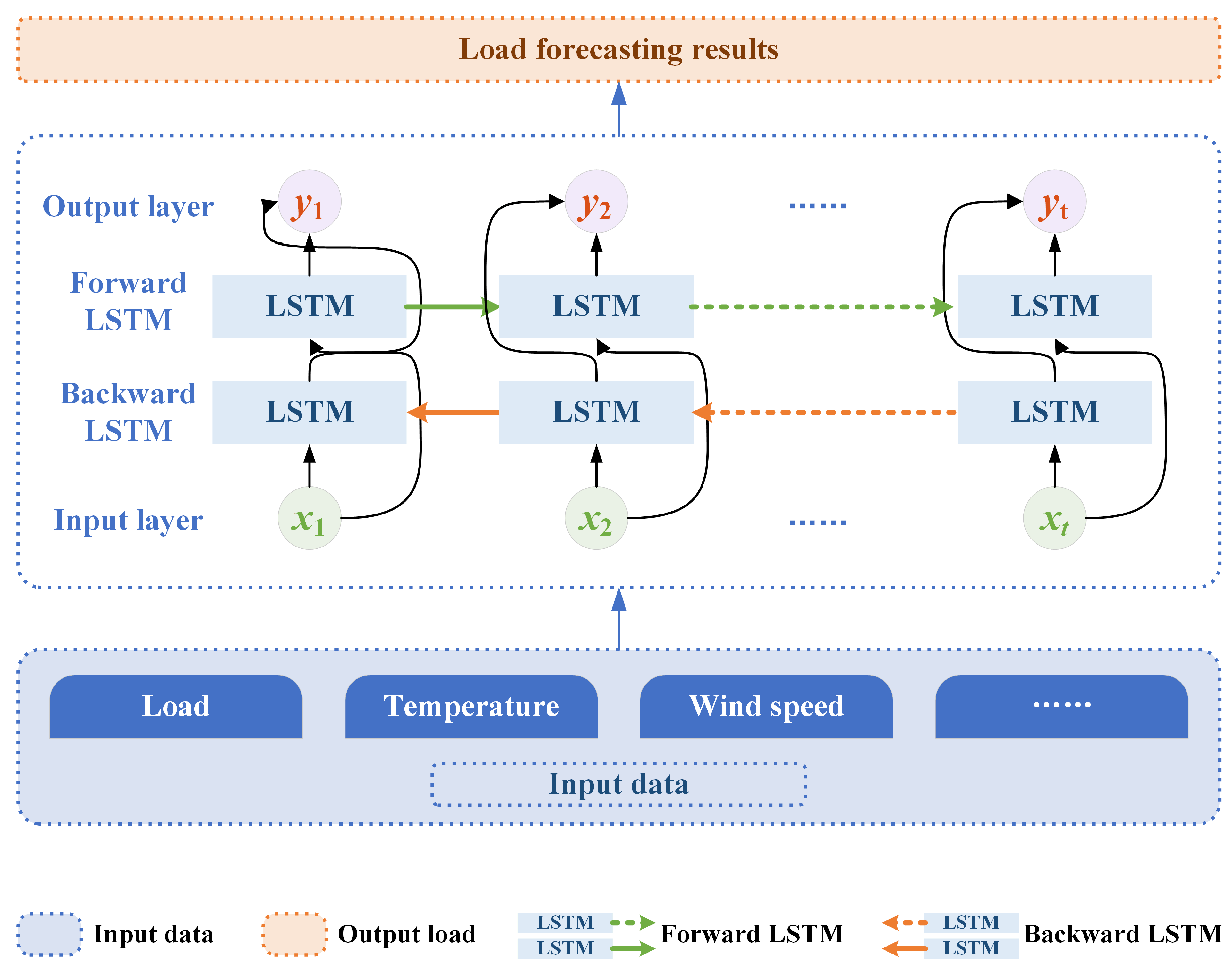
3.1. BiLSTM-Based Load Forecasting Algorithm

The modeling capability is enhanced in BiLSTM by running two independent LSTM networks in each of the two directions of the input sequence, which is able to simultaneously consider the trends and periodicities of different time scales of the load data series, such as short-term fluctuations and long-term trends of the loads, and thus better capture the diversity and complexity of the load data. The computational process is represented as [32]:

$$\left\{\begin{array}{c}{h}_{ti}=LSTM(x_t,h_{ti-1})\\ h_{to}=LSTM(x_t,h_{to-1})\\ y_t={\omega }_t{h}_{ti}+{\nu }_t{h}_{to}+b_y\end{array}\right.$$

(15)

where the forward load feature vector h_ti characterizes the historical load pattern, which is obtained through time series feature extraction of historical load curves. The reverse load feature vector h_to characterizes the context-dependent features of load changes, which is generated by inverse analysis of the potential cyclic characteristics of the load. LSTM(·) denotes the load feature extraction network. ω_t and υ_t denote the time series feature weight and context-dependent feature weight, which quantify the importance of the historical load evolution pattern and load fluctuation correlation features to the current forecast [33].

The power feature weighting mechanism is adopted to the final feature fusion, which realizes the nonlinear coupling of historical load and contextual features of load variations through the feature weight matrix, and provides the fused feature vectors containing multiple power characteristics for the subsequent fully connected layer.

The structure of the load forecasting model is shown in Figure 1, where the processed electricity load, temperature, humidity, wind speed and other influencing factors are used as feature inputs, and the BiLSTM model is used to learn the input features and output the load forecasting results.

3.2. Procedure of Load Forecasting Method Based on QGCT and BiLSTM

The load forecasting model framework considering multiple influencing factors provides a comprehensive approach to improve the accuracy and reliability of electric load forecasting. The framework consists of four key parts: (1) the original data are cleaned and organized to ensure the quality of the data and provide a solid foundation for subsequent analysis; (2) the smoothness test is conducted on both the influencing factors and power load series to determine whether the time series of the data meets the smoothness requirement, which is crucial for the establishment of the forecasting model; (3) the Granger causality test between the influencing factors and load is carried out to identify causal relationships and support the construction of a more accurate prediction model; (4) the BiLSTM-based load forecasting is presented combining the information obtained from the previous analysis.

To implement the framework, the first critical step is data preprocessing. The collected data of electricity load and the data of each environmental factor including temperature, humidity and wind speed are organized to judge whether there is any abnormality or not, and adjust the abnormal data.

Moreover, with clean and organized data, the next step is to verify the statistical properties of the time series. Before conducting the causality test of each influencing factor and load change, the smoothness test of all the series should be conducted first. Comparisons are made based on the ADF statistic and the critical value to determine whether each influencing factor and load time series is smooth or not, and for non-smooth series can be differenced or otherwise transformed to make them smooth, and the series can be used for subsequent load forecasting modeling.

Subsequently, once the smoothness of the data is confirmed, the analysis can proceed to investigate the relationships between variables. For each of the influencing factor series as well as the electricity load series obtained after the above processing, the causal relationships at different quartiles are captured by selecting the quartiles and building regression models of different influencing factors on electricity load for each selected quartile, and the Granger causality test statistic are calculated.

Finally, based on the obtained causal relationships of different factors on load changes, the BiLSTM-based load forecasting model is established. The filtered key influencing factors on load changes are used as input feature quantities to train the model, so as to obtain the load forecasting results.

4. Case Study

In this paper, the daily maximum temperature, minimum temperature, average temperature, maximum relative humidity, minimum relative humidity, average relative humidity, maximum wind speed, minimum wind speed, average wind speed, rainfall and load average data of Fujian, China, for the 273 days from 1 February 2023 to 31 October 2023 are selected as samples for the analysis. The data from February to July are used as the training set, and the data from August to October are used as the test set to analyze the model prediction effect.

4.1. Results of the Causality Test Between Environmental Factors and Electricity Loads

In order to realize the subsequent causality analysis between the electricity load and the various influencing factors, it is first necessary to carry out the ADF smoothness test for the series of maximum temperature, minimum temperature, average temperature, maximum relative humidity, minimum relative humidity, average relative humidity, maximum wind speed, minimum wind speed, average wind speed, rainfall and load mean.

The ADF test results for each feature quantity are shown in

Table 1. ADF test results for the original feature sequence.

Factors	Threshold of 1%	ADF Value	Probability
Maximum temperature	−1.9424	−13.294	0.0010 **
Minimum temperature	−1.9424	−6.8712	0.0010 **
Average temperature	−1.9424	−3.4273	0.0010 **
Maximum humidity	−1.9424	−13.049	0.0010 **
Minimum humidity	−1.9424	−7.4050	0.0010 **
Average humidity	−1.9424	−5.7568	0.0010 **
Maximum wind speed	−1.9424	−13.657	0.0010 **
Minimum wind speed	−1.9424	−6.1659	0.0010 **
Average wind speed	−1.9424	−6.6557	0.0010 **
Rainfall	−1.9424	−8.2339	0.0010 **
Average load	−1.9424	−3.1475	0.0024 **

Note: ** indicates that the item passes the 0.01 level of significance test.

. It can be seen that all the original feature series pass the smoothness test, and the original series is used for causality analysis.

Granger causality tests at different quantile levels were performed using the above characterized series that passed the smoothness test. Nineteen isometric quantiles were obtained in [0.05, 0.95], and the lags were set to be 1 day, 2 days, and 3 days, respectively.

The causality test values of all influential factors on load at different quartiles with the lag of 1 day are demonstrated in

Table 2. Granger causality test values of the influence factors on load at the lag of one day.

Quartile	Maximum Temperature	Minimum Temperature	Average Temperature	Maximum Humidity	Minimum Humidity	Average Humidity	Maximum Wind Speed	Minimum Wind Speed	Average Wind Speed	Rainfall
0.05	0.0071	0.0071	0.0709	0.0071	0.0071	0.3901	0.0071	0.0071	0.2270	0.0071
0.10	0.0071	0.0071	0.7305	0.0071	0.0071	0.0071	0.0071	0.0071	0.0071	0.0071
0.15	0.0071	0.0071	0.2979	0.0071	0.0071	0.0142	0.0071	0.0071	0.1348	0.0071
0.20	0.0071	0.0071	0.0142	0.0071	0.0071	0.5957	0.0071	0.0071	0.1064	0.0071
0.25	0.0071	0.0071	0.0213	0.0071	0.0071	0.7660	0.0071	0.0071	0.2695	0.0071
0.30	0.0071	0.0071	0.0071	0.0071	0.0071	0.7589	0.0071	0.0071	0.0071	0.0071
0.35	0.0071	0.0071	0.0709	0.0071	0.0071	0.2128	0.0071	0.0071	0.0709	0.0071
0.40	0.0071	0.0071	0.0993	0.0071	0.0071	0.2553	0.0071	0.0071	0.0071	0.0071
0.45	0.0071	0.0071	0.1064	0.0071	0.0071	0.0851	0.0071	0.0071	0.3546	0.0071
0.50	0.1773	0.0071	0.0213	0.1631	0.0071	0.0709	0.1135	0.0071	0.4397	0.0071
0.55	0.0355	0.0071	0.3901	0.0355	0.0071	0.8156	0.0426	0.0071	0.3688	0.0071
0.60	0.0071	0.0071	0.4113	0.0071	0.0071	0.3759	0.0071	0.0071	0.6596	0.0071
0.65	0.0071	0.0071	0.1773	0.0071	0.0071	0.9433	0.0071	0.0071	0.7376	0.0071
0.70	0.0071	0.0071	0.0567	0.0071	0.0071	0.8369	0.0071	0.0071	0.1844	0.0071
0.75	0.0071	0.0071	0.2340	0.0071	0.0071	0.0851	0.0071	0.0071	0.0355	0.0071
0.80	0.0071	0.0071	0.2199	0.0071	0.0071	0.0071	0.0071	0.0071	0.0071	0.0071
0.85	0.0071	0.0071	0.3333	0.0071	0.0071	0.2411	0.0071	0.0071	0.0071	0.0071
0.90	0.0071	0.0071	0.0142	0.0071	0.0071	0.3050	0.0071	0.0071	0.0071	0.0071
0.95	0.0071	0.0071	0.0213	0.0071	0.0071	0.4043	0.0071	0.0071	0.5461	0.0071

Note: the bold portion indicates that the item accepts the original hypothesis at the 1% significance level that there is no Granger causality.

. It is observed that average temperature, average relative humidity, and average wind speed do not lead to Granger changes in the average load at the 1% significance level, which suggests that these results are robust to the quantile regression model under the null hypothesis of Granger non-causality. Thus, there is no evidence for Granger causality between changes in average temperature, average relative humidity, and average wind speed and changes in load. In quartiles closer to the top and bottom, temperature, humidity, and wind speed show stronger Granger causality with load changes. This suggests that the model detects more significant causal relations under extreme weather conditions compared to moderate weather changes. While the traditional mean Granger test focuses only on the mean of the conditional distribution, the quantile analysis is able to capture the tail dependencies, highlighting the potential impacts of extreme weather events on electricity loads. Thus, the strength of the quantile framework in identifying key influences is validated, especially in scenarios with sharp load fluctuations or frequent extreme weather events.

Meanwhile, when the maximum temperature, the maximum relative humidity and the maximum wind speed are in the middle of the quantile range, there are a small number of intervals in which there are no obvious causal results. This may be due to the fact that the amount of factor characteristics is at an intermediate level, which produces a diversity of influences on human activities and prevents the formation of a more uniform trend of activities. The unpredictable load changes are created by the decentralization of choices, and evidence of Granger causality is demonstrated when these characteristics undergo larger positive or negative, suggesting that these factors lead to changes in loads.

The causality test values of all influential factors on electricity load at different quartiles for lags of 2 days and 3 days are shown in

Table 3. Granger causality test values of the influence factors on load at the lag of two days.

Quartile	Maximum Temperature	Minimum Temperature	Average Temperature	Maximum Humidity	Minimum Humidity	Average Humidity	Maximum Wind Speed	Minimum Wind Speed	Average Wind Speed	Rainfall
0.05	0.0071	0.0071	0.0709	0.0071	0.0071	0.4610	0.0071	0.0071	0.4681	0.0071
0.10	0.0071	0.0071	0.6170	0.0071	0.0071	0.0071	0.0071	0.0071	0.0638	0.0071
0.15	0.0071	0.0071	0.1844	0.0071	0.0071	0.0213	0.0071	0.0071	0.0071	0.0071
0.20	0.0071	0.0071	0.0071	0.0071	0.0071	0.6950	0.0071	0.0071	0.2270	0.0071
0.25	0.0071	0.0071	0.0071	0.0071	0.0071	0.7021	0.0071	0.0071	0.1844	0.0071
0.30	0.0071	0.0071	0.0496	0.0071	0.0071	0.2411	0.0071	0.0071	0.1560	0.0071
0.35	0.0071	0.0071	0.1844	0.0071	0.0071	0.6809	0.0071	0.0071	0.0284	0.0071
0.40	0.0071	0.0071	0.0638	0.0071	0.0071	0.2624	0.0071	0.0071	0.0213	0.0071
0.45	0.0071	0.0071	0.0284	0.0071	0.0071	0.1206	0.0071	0.0071	0.0426	0.0071
0.50	0.2908	0.0071	0.0071	0.4043	0.0071	0.0213	0.2057	0.0071	0.4184	0.0071
0.55	0.1206	0.0071	0.7872	0.0355	0.0071	0.7092	0.2057	0.0071	0.8652	0.0071
0.60	0.0071	0.0071	0.3759	0.0071	0.0071	0.6738	0.0851	0.0071	0.3688	0.0071
0.65	0.0071	0.0071	0.4610	0.0071	0.0071	0.1560	0.0071	0.0071	0.1631	0.0071
0.70	0.0071	0.0071	0.4681	0.0071	0.0071	0.7518	0.0071	0.0071	0.0922	0.0071
0.75	0.0071	0.0071	0.4610	0.0071	0.0071	0.1560	0.0071	0.0071	0.0426	0.0071
0.80	0.0071	0.0071	0.1915	0.0071	0.0071	0.7447	0.0071	0.0071	0.0142	0.0071
0.85	0.0071	0.0071	0.3404	0.0071	0.0071	0.5035	0.0071	0.0071	0.0071	0.0071
0.90	0.0071	0.0071	0.2057	0.0071	0.0071	0.0071	0.0071	0.0071	0.0213	0.0071
0.95	0.0071	0.0071	0.1348	0.0071	0.0071	0.5887	0.0071	0.0071	0.7801	0.0071

Note: the bold portion indicates that the item accepts the original hypothesis at the 1% significance level that there is no Granger causality.

and

Table 4. Granger causality test values of the influence factors on load at the lag of three days.

Quartile	Maximum Temperature	Minimum Temperature	Average Temperature	Maximum Humidity	Minimum Humidity	Average Humidity	Maximum Wind Speed	Minimum Wind Speed	Average Wind Speed	Rainfall
0.05	0.0071	0.0071	0.0355	0.0071	0.0071	0.4610	0.0071	0.0071	0.4326	0.0071
0.10	0.0071	0.0071	0.6596	0.0071	0.0071	0.1064	0.0071	0.0071	0.0567	0.0071
0.15	0.0071	0.0071	0.1844	0.0071	0.0071	0.0071	0.0071	0.0071	0.1702	0.0071
0.20	0.0071	0.0071	0.0071	0.0071	0.0071	0.6879	0.0071	0.0071	0.1064	0.0071
0.25	0.0071	0.0071	0.0071	0.0071	0.0071	0.3333	0.0071	0.0071	0.1489	0.0071
0.30	0.0071	0.0071	0.0709	0.0071	0.0071	0.7092	0.0071	0.0071	0.0426	0.0071
0.35	0.0071	0.0071	0.0496	0.0071	0.0071	0.0993	0.0071	0.0071	0.1418	0.0071
0.40	0.0071	0.0071	0.0496	0.0071	0.0071	0.2695	0.0071	0.0071	0.2128	0.0071
0.45	0.0071	0.0071	0.0284	0.0071	0.0071	0.2553	0.0071	0.0071	0.1348	0.0071
0.50	0.0567	0.0071	0.0426	0.1206	0.0071	0.6879	0.2979	0.0071	0.3688	0.0071
0.55	0.0993	0.0071	0.9078	0.1206	0.0071	0.2695	0.1773	0.0071	0.7660	0.0071
0.60	0.0071	0.0071	0.8085	0.0071	0.0071	0.1986	0.0496	0.0071	0.6241	0.0071
0.65	0.0071	0.0071	0.0851	0.0071	0.0071	0.0638	0.0071	0.0071	0.4823	0.0071
0.70	0.0071	0.0071	0.4681	0.0071	0.0071	0.8794	0.0071	0.0071	0.0071	0.0071
0.75	0.0071	0.0071	0.4184	0.0071	0.0071	0.9504	0.0071	0.0071	0.2908	0.0071
0.80	0.0071	0.0071	0.2128	0.0071	0.0071	0.6950	0.0071	0.0071	0.0071	0.0071
0.85	0.0071	0.0071	0.3121	0.0071	0.0071	0.1064	0.0071	0.0071	0.0071	0.0071
0.90	0.0071	0.0071	0.2624	0.0071	0.0071	0.2837	0.0071	0.0071	0.0142	0.0071
0.95	0.0071	0.0071	0.1631	0.0071	0.0071	0.5745	0.0071	0.0071	0.6170	0.0071

Note: the bold portion indicates that the item accepts the original hypothesis at the 1% significance level that there is no Granger causality.

, respectively, and the general distributions are similar to those of Table 2, with some variations in the test values. The trend consistency of the results for different lags can indicate that the causal relationship of the characteristic changes on load is stable under different lag lengths. In other words, no matter how long the lag is chosen for the analysis, the load is affected the change in characteristics in a consistent manner. This consistency indicates that the causal relationship is robust across lags and is not affected by lag length.

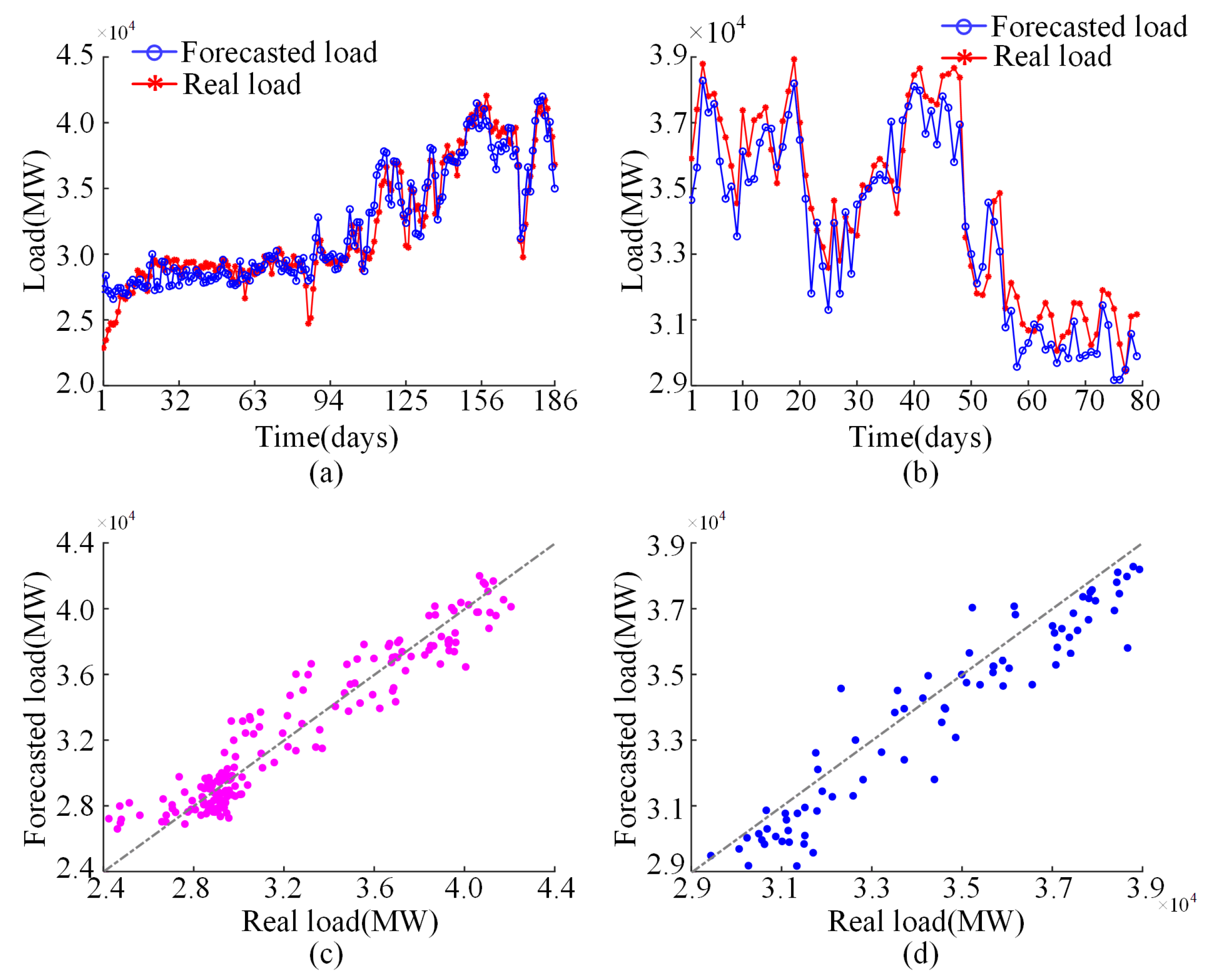
4.2. Effectiveness Analysis of QGCT-BiLSTM for Load Forecasting

The comparative analysis is used in this study to analyze the superiority of the load forecasting model. The first stage is constructed to incorporate all influential factors not analyzed by causal correlation into the input feature set for load forecasting. The training set fitting load curve and test set prediction load curve are shown in Figure 2a,b. The basic fitting properties is presented during the training stage, but the test set scatter point distribution reveals that there are abnormal deviations in the results as shown in Figure 2c,d, and about 37.97% of the test samples show a relative error of more than ±15%.

The second stage was implemented as a causality-based feature screening mechanism that retained only those influences that had significant association with load changes. The key factors affecting the load variations are screened out including: maximum temperature, minimum temperature, maximum relative humidity, minimum relative humidity, maximum wind speed, minimum wind speed and rainfall. These key influencing factors are used as input features to realize the forecasting of load. The fitted load curve of the training set and test set with the improved model are shown in Figure 3a,b. The scatter distributions show tighter linear aggregation characteristics as shown in Figure 3c,d. The comparative analysis shows that the curve shape of the model after feature screening agrees significantly with the measured load trend, and the percentage of samples exceeding ±15% relative error decreases by 11.39%.

To evaluate the differences further quantitatively in prediction performance, a four-dimensional assessment system containing root mean square error (RMSE), mean absolute error (MAE), mean bias error (MBE) and mean absolute percentage error (MAPE) is established. As shown in

Table 5. Evaluation metrics for evaluating load forecasting results before and after filtering key influencing factors.

Evaluation Metrics	Unfiltered		Filtered
	Training Set	Test Set	Training Set	Test Set
RMSE	187.91	205.15	105.81	145.27
MAE	136.05	162.49	87.60	113.65
MBE	1.89	−95.56	7.49	−61.61
MAPE	0.0432	0.0469	0.0366	0.0255

, the test set prediction errors of the model after feature screening show a systematic decrease: the relative decrease of RMSE, MAE and MAPE are 29.19%, 30.06% and 45.63%. The directional correction of MBE is 35.53%. The improved consistency of the indicators confirms that causal feature screening effectively reduces the noise interference of spurious-correlated variables, enabling the model to capture the essential driving mechanisms of load changes more accurately.

Moreover, the key factors screened by the Granger causality test significantly reduced the forecast errors. The decreases in RMSE and MAE indicate that the exclusion of low-correlation variables reduces the risk of overfitting the model to noise. The large decrease in MAPE further suggests that the screened feature set is more attuned to the driving mechanisms of load changes. For example, maximum temperature as a key factor is directly associated with the peak demand of air conditioning loads in summer, while the inclusion of rainfall may reflect the short-term dampening effect of stormy weather on industrial electricity consumption. This result validates the center role of causal feature screening in enhancing model generalization capabilities.

4.3. Superiority Analysis of QGCT-BiLSTM for Load Forecasting

The proposed QGCT-BiLSTM method is rigorously evaluated against other load forecasting techniques, including Back Propagation (BP) Neural Network [34], Convolutional Neural Networks (CNN) [35], Long Short-Term Memory (LSTM) [36] and Random Forest (RF) [37], to validate its superiority in both regression and time-series forecasting frameworks. The evaluation of errors in load forecasting results of different methods are shown in

Table 6. Evaluation of errors in load forecasting results of different methods.

Category	Method		RMSE	MAE	MAPE
Regression load forecasting	Unfiltered Key Factors	BP [34]	192.5175	160.7176	0.0465
		CNN [35]	193.9727	157.0710	0.0460
		LSTM [36]	190.8181	155.0108	0.0443
		RF [37]	188.6064	160.7783	0.0472
		QGCT-BiLSTM	205.1504	162.4930	0.0469
	Filtered Key Factors	BP [34]	170.2113	141.0954	0.0413
		CNN [35]	181.3503	155.6983	00455
		LSTM [36]	172.0750	137.7569	0.0399
		RF [37]	185.5207	160.2694	0.0471
		QGCT-BiLSTM	145.2686	113.6537	0.0255
Time-series load forecasting	BP [34]		321.8326	276.0081	0.0779
	CNN [35]		429.9377	356.0354	0.1027
	LSTM [36]		364.3561	297.9974	0.0834
	RF [37]		300.4929	261.7523	0.0740

. Comparative analyses are conducted under two distinct scenarios: regression forecasting with filtered/unfiltered key factors and pure time-series forecasting without external influencing variables. This dual approach ensured a comprehensive assessment of the QGCT-BiLSTM’s adaptability.

The significant advancements in load forecasting accuracy are demonstrated by the proposed QGCT-BiLSTM method, as evidenced by the superior performance across critical error metrics compared to conventional approaches. Under the regression load forecasting framework with filtered key factors, QGCT-BiLSTM achieves remarkably low errors, outperforming all baseline methods including BP, CNN, LSTM and RF. Moreover, The RMSE and MAE values of QGCT-BiLSTM are 20.3% and 16.8% lower than the next best method (LSTM) in the same category, respectively. This substantial improvement underscores the efficacy of integrating bidirectional long short-term memory (BiLSTM) with the QGCT mechanism.

Furthermore, the analysis reveals that QGCT-BiLSTM benefits significantly from the utilization of filtered key factors. When compared to the performance of QGCT-BiLSTM under unfiltered conditions, the adoption of filtered factors reduces prediction errors by 29.2% (RMSE), 30.1% (MAE) and 45.6% (MAPE), respectively, highlighting the critical role of feature selection in eliminating noise and irrelevant variables. In contrast, traditional methods such as BP and RF exhibit limited sensitivity to factor filtering, with error reductions of only 11.6–12.8% (RMSE) and 0.3–1.5% (MAPE). This QGCT-BiLSTM’s robustness is emphasized by the disparity in leveraging refined input data to optimize model generalizability.

Compared to the results of forecasting using only load data, BP, CNN, LSTM and RF compared to QGCT reduced the average of all errors by 60.32%, 69.82%, 63.81% and 57.63%, respectively, which proves the importance of introducing climatic influences for forecasting load changes.

4.4. Sensitivity Analysis of Load Influencing Factors at Seasonal Scales

In order to verify the sensitivity of the load forecast results to each environmental factor, which is characterized by the error in the load forecast results after the change in characteristics by sequentially varying the individual climate factor data to 10% of the true data. Meanwhile, in order to combine the local geographic features and living habits of the residents more closely, the data are analyzed according to the seasonal scale, in which February, March, April and May are in spring, June, July and August are in summer, and September and October are in autumn. The distribution of load forecasting errors due to changes in climate characteristics at the seasonal scale is shown in Figure 4. The screened seven key influences are synthesized as temperature, humidity, wind speed and rainfall to simplify the analysis. The different seasons in Figure 4 correspond to bars with different patterns, and specific values are labeled above the bars corresponding to the different factors for each season to make the results clearer.

With a subtropical monsoon climate and four distinct seasons, the Fujian region has more extreme weather such as typhoons in summer and windy spring and autumn, and is located on the southeast coast with a pronounced oceanic climate. The unique geographic location and climate characteristics have a significant impact on load changes.

The sensitivities of the load forecast to changes in the influencing factors during spring are humidity, wind speed, temperature and rainfall in descending order. This is due to the fact that Fujian province of China is in the early part of the rainy season at this time with high humidity and increased demand for dehumidification equipment from residents, resulting in load sensitivity to changes in humidity. Higher wind speeds in spring lead to significant load changes in wind power equipment especially in coastal areas. Also, the moderate temperatures and rainfall in the spring had a limited impact on residential and industrial electricity consumption.

The sensitivities of load forecasts to changes in influencing factors during summer are temperature, rainfall, wind speed and humidity in descending order. The high temperatures in Fujian province of China during summer lead to a surge in demand for cooling by residents, resulting in loads that are highly sensitive to changes in temperature. Moreover, summer is the season of heavy rainfall and typhoons, which have a greater impact on the demand for electricity for residents and industrial activities. Residents are less concerned about humidity in the summer resulting in lower load sensitivity to humidity.

The sensitivities of load forecasts to changes in influencing factors during autumn are temperature, wind speed, rainfall and humidity in descending order. The temperature is still at a high level at the beginning of autumn and the temperature drops at night in Fujian province of China. Thus, the demand for electricity from residents is sensitive to temperature changes. Furthermore, wind speed is higher in autumn, and the load of wind power equipment increases. Reduced rainfall as well as moderate humidity in autumn have less impact on residential and industrial electricity consumption.

5. Conclusions

A power load forecasting framework integrating QGCT and BiLSTM is proposed in this paper. The technical advantages of the method are verified through a systematic empirical study, and the main conclusions are as follows:

(1) The Granger causality testing mechanism based on quantile regression framework can effectively identify the association between meteorological factors and load. The method screens out the core set of influencing factors with stable causal relationships as inputs to the prediction model through significance test to improve the accuracy of prediction.

(2) Improvement effects of feature screening on load forecasting model performance are quantitatively demonstrated by the results of the error assessment system. The comparative study validates the critical role of causal feature selection in load forecasting. The average reduction in the error metrics reached 34.96% and the correction in MBE reached 35.53%.

(3) The sensitivity characteristics of load forecasting to key meteorological parameters at seasonal scales are revealed, providing a theoretical basis for the establishment of load forecasting models with seasonal dependence.

This paper provides theoretical support and practical tools for intelligent operation of power systems through mechanism explanation and quantitative analysis. Meanwhile, this study focuses on a single region with limited time series. Future work could expand to multi-year, multi-regional datasets, integrate probabilistic forecasting, and investigate advanced architectures such as transformers and explore multi-regional data synergy and long-term predictive modeling of extreme climate events to address the energy management challenges in application domains such as utility companies and smart grids.

References

1. Guo, W.Y.; Liu, S.J.; Weng, L.G.; Liang, X.Y. Power grid load forecasting using a CNN-LSTM network based on a multi-model attention mechanism. Appl. Sci. 2025, 15, 2435. [Google Scholar] [CrossRef]
2. Chen, J.Y.; Liu, L.S.; Guo, K.Q.; Liu, S.R.; He, D.W. Short-term electricity load forecasting based on improved data decomposition and hybrid deep-learning models. Appl. Sci. 2024, 14, 5966. [Google Scholar] [CrossRef]
3. Zhou, Z.Y.; Ren, C.; Xu, Y. Forecasting masked-load with invisible distributed energy resources based on transfer learning and Bayesian tuning. Energy Convers. Econ. 2024, 5, 316–326. [Google Scholar] [CrossRef]
4. Dong, H.J.; Zhu, J.Z.; Li, S.L.; Miao, Y.W.; Chung, C.Y.; Chen, Z.Y. Probabilistic residential load forecasting with sequence-to-sequence adversarial domain adaptation networks. J. Mod. Power Syst. Clean Energy 2024, 12, 1559–1571. [Google Scholar] [CrossRef]
5. Chen, C.M.; Li, Y.; Qiu, W.Q.; Liu, C.; Zhang, Q.; Li, Z.Y.; Lin, Z.Z.; Yang, L. Cooperative-game-based day-ahead scheduling of local integrated energy systems with shared energy storage. IEEE Trans. Sustain. Energy 2022, 13, 1994–2011. [Google Scholar] [CrossRef]
6. Chen, C.M.; Zhu, Y.Q.; Zhang, T.H.; Li, Q.S.; Li, Z.; Liang, H.L.; Liu, C.; Ma, Y.Q.; Lin, Z.Z.; Yang, Y. Two-stage multiple cooperative games-based joint planning for shared energy storage provider and local integrated energy systems. Energy 2023, 284, 129114. [Google Scholar] [CrossRef]
7. Zhu, J.Z.; Miao, Y.W.; Dong, H.J.; Li, S.L.; Chen, Z.Y.; Zhang, D. Short-term residential load forecasting based on k-shape clustering and domain adversarial transfer network. J. Mod. Power Syst. Clean Energy 2024, 12, 1239–1249. [Google Scholar]
8. Waseem, M.; Lin, Z.Z.; Yang, L. Data-driven load forecasting of air conditioners for demand response using Levenberg-Marquardt algorithm-based ANN. Big Data Cogn. Comput. 2019, 3, 36. [Google Scholar] [CrossRef]
9. Ye, C.J.; Ding, Y.; Wang, P.; Lin, Z.Z. A data-driven bottom-up approach for spatial and temporal electric load forecasting. IEEE Trans. Power Syst. 2019, 34, 1966–1979. [Google Scholar] [CrossRef]
10. Zhao, P.; Ling, G.; Song, X.X. ELFNet: An effective electricity load forecasting model based on a deep convolutional neural network with a double-attention mechanism. Appl. Sci. 2024, 14, 6270. [Google Scholar] [CrossRef]
11. Tang, B.B.; Hu, J.; Yang, M.; Zhang, C.L.; Bai, Q. Enhancing short-term load forecasting accuracy in high-volatility regions using lstm-scn hybrid models. Appl. Sci. 2024, 14, 11606. [Google Scholar] [CrossRef]
12. Luo, J.; Hong, T.; Fang, S.C. Robust regression models for load forecasting. IEEE Trans. Smart Grid 2019, 10, 5397–5404. [Google Scholar] [CrossRef]
13. Richter, L.; Lenk, S.; Bretschneider, P. Advancing electric load forecasting: Leveraging federated learning for distributed, non-stationary, and discontinuous time series. Smart Cities 2024, 7, 2065–2093. [Google Scholar] [CrossRef]
14. Zheng, Z.; Chen, H.N.; Luo, X.W. A Kalman filter-based bottom-up approach for household short-term load forecast. Appl. Energy 2019, 250, 882–894. [Google Scholar] [CrossRef]
15. Dudek, G.; Pelda, P.; Smyl, S. A hybrid residual dilated lstm and exponential smoothing model for midterm electric load forecasting. IEEE Trans. Neural Netw. Learn. Syst. 2022, 33, 2879–2891. [Google Scholar] [CrossRef]
16. Wu, D.; Wang, B.Y.; Precup, D.; Boulet, B. Multiple kernel learning-based transfer regression for electric load forecasting. IEEE Trans. Smart Grid 2020, 11, 1183–1192. [Google Scholar] [CrossRef]
17. Wang, C.; Zhao, H.S.; Liu, Y.; Fan, G.J. Minute-level ultra-short-term power load forecasting based on time series data features. Appl. Energy 2024, 372, 123801. [Google Scholar] [CrossRef]
18. Sharma, S.; Majumdar, A.; Elvira, V.; Chouzenoux, E. Blind Kalman filtering for short-term load forecasting. IEEE Trans. Power Syst. 2020, 35, 4916–4919. [Google Scholar] [CrossRef]
19. Smyl, S.; Dudek, G.; Pelka, P. ES-dRNN: A hybrid exponential smoothing and dilated recurrent neural network model for short-term load forecasting. IEEE Trans. Neural Netw. Learn. Syst. 2024, 35, 11346–11358. [Google Scholar] [CrossRef]
20. Lin, W.X.; Wu, D.; Boulet, B. Spatial-temporal residential short-term load forecasting via graph neural networks. IEEE Trans. Smart Grid 2021, 12, 5373–5384. [Google Scholar] [CrossRef]
21. Ramos, D.; Faria, P.; Vale, Z.; Correia, R. Short time electricity consumption forecast in an industry facility. IEEE Trans. Ind. Appl. 2022, 58, 123–130. [Google Scholar] [CrossRef]
22. Huang, C.H.; Bu, S.R.; Chen, W.L.; Wang, H.; Zhang, Y.R. Deep reinforcement learning-assisted federated learning for robust short-term load forecasting in electricity wholesale markets. IEEE Trans. Netw. Sci. Eng. 2024, 11, 5073–5086. [Google Scholar] [CrossRef]
23. Wang, H.; Zhang, N.; Du, E.; Yan, J.; Han, S.; Liu, Y.Q. A comprehensive review for wind, solar, and electrical load forecasting methods. Glob. Energy Interconnect. 2022, 5, 9–30. [Google Scholar] [CrossRef]
24. Sharma, A.; Jain, S.K. A Novel two-stage framework for mid-term electric load forecasting. IEEE Trans. Ind. Inform. 2024, 20, 247–255. [Google Scholar] [CrossRef]
25. Chen, K.J.; Chen, K.L.; Wang, Q.; He, Z.Y.; Hu, J.; He, J.L. Short-term load forecasting with deep residual networks. IEEE Trans. Smart Grid 2019, 10, 3943–3952. [Google Scholar] [CrossRef]
26. Dai, Y.M.; Zhao, P. A hybrid load forecasting model based on support vector machine with intelligent methods for feature selection and parameter optimization. Appl. Energy 2020, 279, 115332. [Google Scholar] [CrossRef]
27. Zhang, W.Y.; Chen, Q.; Yan, J.Y.; Zhang, S.; Xu, J.Y. A novel asynchronous deep reinforcement learning model with adaptive early forecasting method and reward incentive mechanism for short-term load forecasting. Energy 2021, 236, 121492. [Google Scholar] [CrossRef]
28. Ludwig, N.; Arora, S.; Taylor, J.W. Probabilistic load forecasting using post-processed weather ensemble predictions. J. Oper. Res. Soc. 2023, 74, 1008–1020. [Google Scholar] [CrossRef]
29. Sobhani, M.; Campbell, A.; Sangamwar, S.; Li, C.L.; Hong, T. Combining weather stations for electric load forecasting. Energies 2019, 12, 1510. [Google Scholar] [CrossRef]
30. Li, B.W.; Zhang, J.; He, Y.; Wang, Y. Short-term load-forecasting method based on wavelet decomposition with second-order gray neural network model combined with ADF test. IEEE Access 2017, 5, 16324–16331. [Google Scholar] [CrossRef]
31. Troster, V.; Shahbaz, M.; Uddin, G.S. Renewable energy, oil prices, and economic activity: A Granger-causality in quantiles analysis. Energy Econ. 2018, 70, 440–452. [Google Scholar] [CrossRef]
32. Wu, K.L.; Gu, J.; Meng, L.; Wen, H.L.; Ma, J.H. An explainable framework for load forecasting of a regional integrated energy system based on coupled features and multi-task learning. Prot. Control Mod. Power Syst. 2022, 7, 24. [Google Scholar] [CrossRef]
33. Zhu, S.X.; Ma, H.R.; Chen, L.J.; Wang, B.; Wang, H.X.; Li, X.Z.; Gao, W.Z. Short-term load forecasting of an integrated energy system based on STL-CPLE with multitask learning. Prot. Control Mod. Power Syst. 2024, 9, 71–92. [Google Scholar] [CrossRef]
34. Fan, G.F.; Guo, Y.H.; Zheng, J.M.; Hong, W.C. A generalized regression model based on hybrid empirical mode decomposition and support vector regression with back-propagation neural network for mid-short-term load forecasting. J. Forecast. 2020, 39, 737–756. [Google Scholar] [CrossRef]
35. Aslam, S.; Ayub, N.; Farooq, U.; Alvi, M.J.; Albogamy, F.R.; Rukh, G.; Haider, S.I.; Azar, A.T.; Bukhsh, R. Towards electric price and load forecasting using CNN-based ensembler in smart grid. Sustainability 2021, 13, 12653. [Google Scholar] [CrossRef]
36. Zhang, Z.D.; Qin, H.; Yan, L.Q.; Lu, J.Y.; Cheng, L.G. Interval prediction method based on long-short term memory networks for system integrated of hydro, wind and solar power. Energy Procedia 2019, 158, 6176–6182. [Google Scholar] [CrossRef]
37. Aprillia, H.; Yang, H.T.; Huang, C.M. Statistical load forecasting using optimal quantile regression random forest and risk assessment index. IEEE Trans. Smart Grid 2021, 12, 1467–1480. [Google Scholar] [CrossRef]
Figure 1. The structure diagram of load forecasting model based on BiLSTM.
Applsci 15 05912 g001
Figure 2. Load forecasting results for unfiltered key factors: (a) training set load curve; (b) test set load curve; (c) scatterplot of training set; (d) scatterplot of test set.
Applsci 15 05912 g002
Figure 3. Load forecasting results for filtered key factors: (a) training set load curve; (b) test set load curve; (c) scatterplot of training set; (d) scatterplot of test set.
Applsci 15 05912 g003
Figure 4. Distribution of load forecast errors due to changes in climate characteristics at seasonal scales.
Applsci 15 05912 g004