Featured Application
There are many examples of situations in which scientific knowledge discovered or produced in mathematics has not only turned into very important scientific input for another scientific discipline but has also triggered the practical production of another scientific discipline. In this context, it can be said that the theoretical framework of mathematics has been the subject of extensive application in scientific disciplines such as engineering, health, finance, and education. Machine learning methods, constituting one of the leading tools in the applied sciences, are also built on mathematical foundations. By analyzing large and complex data sets with machine learning methods, it is possible to perform prediction, classification, and decision-making processes effectively without human intervention. In this way, machine learning offers a wide range of applications in daily life, including the automation of processes, early diagnosis of diseases, prevention of financial fraud, management of autonomous systems, and even the shaping of new educational paradigms, forms, and curricula for education.
Abstract
Machine learning makes significant contributions in many areas of the applied sciences. One of these is the field of education, in the form of predicting students’ academic success and developing educational policies. In this study, two distance and kernel-based methods and eight tree-based and ensemble learning models were used to predict students’ academic success. The data set used in the study includes various variables, such as demographic information, academic information, course participation rates, and activity participation status, for 2392 students. Hyperparameter optimization was performed using genetic algorithm and grid search methods and model accuracy was tested with 10-fold cross-validation. In addition, the performances of all machine learning models were compared, using seventeen metric results for three cases, including results without hyperparameter optimization and determinations after hyperparameter optimization. Subsequent to the analyses performed, it was concluded that the SVR, GBM, and XGBoost methods have both high explanatory power and low error rates in regression problems requiring high accuracy, such as analyses aimed at predicting student success.
1. Introduction
Individual differences in education and the multivariate nature of the learning process make it difficult to predict students’ academic performance. While traditional measurement and evaluation methods may be insufficient in determining student achievement, machine learning techniques can make more accurate predictions by modeling complex relationships on large data sets. In this respect, predicting student academic performance is an important research area that contributes to the development of increasingly well-informed educational policies and individualized teaching methods. There are various studies in the literature in which machine learning methods are used to predict student achievement.
In [1], Yağcı compared the performances of machine learning algorithms such as random forest, k-nearest neighbors, support vector machines, logistic regression, and naive Bayes to predict students’ final exam success. Ting et al. evaluated the decision tree, support vector machines, random forest, logistic regression, and k-nearest neighbors algorithms in the context of supervised learning methods to predict student success in higher education [2]. In addition to Ting’s work, Villar and Andrade have evaluated ensemble methods such as gradient boosting, extreme gradient boosting, light gradient boosting, and unbiased boosting with categorical features in their study, in which they used supervised learning methods to predict student success and dropout rates in higher education [3]. In another study, by Alkan, seven different machine learning methods were applied to predict students’ exam success using a publicly available data set called “Student Performance in Exams” [4].
In [5], Bayırbağ and Bakır used machine learning algorithms to predict employee attrition and examined hyperparameter tuning processes. They obtained their best results with the logistic regression model. Farooq et al. proposed a federative learning model for the prediction of student grades and performed a comparative analysis with traditional machine learning methods. Using an approach that differed from the others, they improved their model’s performance by using grid search and genetic algorithm methods in a hyperparameter optimization process [6]. Also, Yang and Shami investigated the effects of hyperparameter optimization of machine learning algorithms on model performance in [7].
Cordovilla et al. used four machine learning models to predict academic success using data associated with 591 students; the data were preprocessed to address class imbalance using the synthetic minority oversampling technique. In their work, they used grid search with cross-validation to train and optimize the models [8].
In [9], Zou et al. explored a population of students majoring in computer science at a specific university and conducted an exploration using their grades in multiple undergraduate courses. The researchers used multiple machine learning models to make regression predictions of student performance. Moreover, Asgarkhani et al. provided a machine learning-based estimation model used for predicting the maximum interstory drift ratio, residual interstory drift ratio, and seismic performance curves of special movement-resisting frames, considering the effect of soil type, in [10].
Some studies on hyperparameter optimization in the context of educational data mining can be described as follows. Wang et al. suggested a novel framework for building a fine-grained performance prediction model with deep neural network architecture, named the adaptive sparse self-attention network (AS-SAN), in [11].
Huang and Chen proposed a new academic performance prediction model (APP-TGN) based on temporal graph neural networks. Moreover, they developed a global sampling module to reduce the problem of false correlation in deep learning-based models in [12].
Huang and Zeng, in [13], suggested a model that uses an interaction-based graph neural network module to learn local academic performance representations from online interaction activities and an attribute-based graph neural network to learn global academic performance representations from the attribute features of all students, by using dynamic graph convolution operations. Wang et al. proposed two novel approaches, namely, Conv-GRU and P-xNN, to predict students’ learning performance and explain the predicted results in [14].
In this study, k-nearest neighbors, support vector regressor, decision tree, random forest, adaptive boosting algorithm, extra trees regressor, gradient boosting regressor, bagging regressor, histogram-based gradient boosting regressor, and extreme gradient boosting methods are used to predict students’ academic performance. In the modeling process, variables such as students’ demographic information, academic performance, and attendance rates were evaluated. The main objective of this study is to compare the prediction success of different machine learning algorithms and determine the best model. In order to improve the performance of machine learning algorithms and minimize the risk of model overfitting, hyperparameter optimization was performed. Hyperparameter optimization ensures that the most appropriate values of certain parameters are selected, in order to ensure the best performance of the model. In this study, hyperparameter optimization is performed using a genetic algorithm and with the use of grid search methods. With the genetic algorithm method, which is inspired by evolutionary computational techniques, natural selection, mutation, and crossover mechanisms are used to determine the optimal hyperparameter combination. The grid search method aims to find the best parameter combination by systematically searching within predetermined hyperparameter ranges. The models were retrained using the best hyperparameter combinations determined for each model, and their overall performances were evaluated using 10-fold cross-validation. The optimization process played a critical role in improving the success of machine learning algorithms on training data sets, especially by revealing how small changes in hyperparameter selection impact model accuracy.
Besides these methods, the performance of machine learning models is evaluated using the metrics of the determination coefficient, mean absolute error, mean squared error, root mean squared error, mean squared error, mean squared log error, maximum error, explained variance, and ten additional metrics. Thus, by analyzing the performance of the hyperparameter-optimized machine learning algorithms, their applicability relative to different data sets can be evaluated.
This study aims to provide a decision support mechanism for predicting student achievement in educational institutions. By providing a reference model for the prediction of the potential success of students in educational institutions, it contributes to a more effective adaptation of teaching strategies. It provides educational administrators with a decision support mechanism that can be used for the early identification of students at risk of low performance and the provision of necessary academic support. By emphasizing the benefits of the effective application of educational data mining methods, it guides future academic-achievement prediction studies. Considering that the existing models for success prediction in education are mostly evaluated with default parameters, and the effect of hyperparameter optimization on model success has infrequently been examined, this study aims to fill this gap by comparatively applying multiple optimization methods.
In the following section, the machine learning models used in this study are explained, and in the third section, the data and the data preprocessing method are given. In the fourth section, hyperparameter optimization techniques and model comparisons are discussed in detail. The results are presented in the fifth section, together with relevant implications for improving the training processes, and suggestions for future research will be developed as well.
2. Machine Learning Methods
In this study, ten different machine learning models are applied to predict students’ academic achievement. The algorithms are classified into two main groups, based on their structural similarities and learning strategies: distance and kernel-based methods, and tree-based and ensemble learning models.
2.1. Distance and Kernel-Based Methods
The k-nearest neighbors (K-NNs) algorithm is a simple and intuitive machine learning algorithm that is widely used in both classification and regression problems. It makes predictions based on similarities between observations. The algorithm calculates the distances between data points, selects the k nearest neighbors, and assigns the class most commonly associated with these neighbors as the class of a new data point. After selecting the data point to be classified or predicted, the distance from this point to every data point in the training data set is calculated. Then, k observations are selected, and the class or value of the data point is predicted by considering the dependent variables of these selected observations [15].
The support vector regressor (SVR) is a powerful regression technique that aims to keep errors within a certain tolerance and can model complex, nonlinear relationships with kernel functions. It provides successful results, especially with high-dimensional and small-sample data sets [16].
2.2. Tree-Based and Ensemble Learning Models
Decision tree (DT) is a versatile machine learning algorithm that can successfully perform classification and regression tasks. It is also a machine learning algorithm that is adaptable to multi-output tasks, has the ability to model complex data sets, and has simple applicability. To build a decision tree, the algorithm iteratively splits the data into smaller and more homogeneous subsets. The partitioning process is performed by selecting a feature that best separates the data set at each step. This process continues until leaf nodes are obtained [17].
The random forest (RF) algorithm is a multi-directional machine learning algorithm that combines multiple decision trees with the ensemble method. This algorithm can solve both classification and regression problems. It divides the training data set into n subsets and predicts between these decision trees by installing a decision-tree algorithm in each cluster [18].
The adaptive boosting (AdaBoost) algorithm is an ensemble learning method used to obtain a stronger model by successively training weak learners in regression problems. Adaptive boosting basically aims to correct errors by giving more weight to incorrectly predicted instances at each iteration [19].
The gradient boosting regressor (GBM) algorithm is a powerful ensemble learning method that combines successively generated weak learners (usually decision trees) to minimize errors. It is particularly effective in regression problems requiring high accuracy, given its progressive error correction structure [20].
The extra trees regressor (ETR) algorithm generates predictions by averaging a large number of decision trees, similar to random forest; however, it can provide lower variance and faster training time due to its completely randomized selection of attribute separation when building trees [21].
The bagging regressor (BR) method trains separate models on multiple subsets generated by random samples from the data set and averages their outputs. In this way, model variance is reduced, and more stable and generalizable predictions are obtained [22].
The histogram-based gradient boosting regressor (HGBR) algorithm divides the continuous variables into histograms during the preprocessing phase of the data set, allowing the model to run faster and with more memory efficiency. This structure is especially optimal for large-scale data sets [23].
The extreme gradient boosting (XGBoost) is a high-performance gradient boosting algorithm that includes advanced features such as regularization and parallel computing. It is one of the preferred methods in many machine learning competitions, due to its robustness in the contexts of extreme learning and computational efficiency [24].
3. Data Set and Preprocessing Steps
In this study, we considered the “Student_performance_data_.csv” data set from the Kaggle platform, representing the academic achievement of students and created to examine the relationship between students’ academic achievement and different variables [25]. This data set is used to analyze the factors affecting students’ academic performance, and it consists of a total of 2392 points of data, which include demographic information, such as the age and gender of the students; academic information, including the frequency of attendance and course study time; and activity participation information, including participation in sports, music, or volunteer activities. In this study, the overall Grade Point Average (GPA) of the student was determined to be the dependent variable, and was the target to be estimated. Grade class was not included in the analysis since it expresses the same concept as GPA. As it is a variable that repeats the same information, it was thought that it might consume unnecessary space in the model and cause overfitting problems. Student ID was not included in the analysis, because it is a unique identifier that identifies the student and has no explanatory function relative to academic performance.
Correlation analysis was performed to evaluate the relationships between the variables in the data set. As a result of the correlation analysis, the heat map of which is given in Figure 1, high linear correlation was found between some variables. Since this may lead to overfitting of the model, some of the variables with high correlation were removed from the data set.
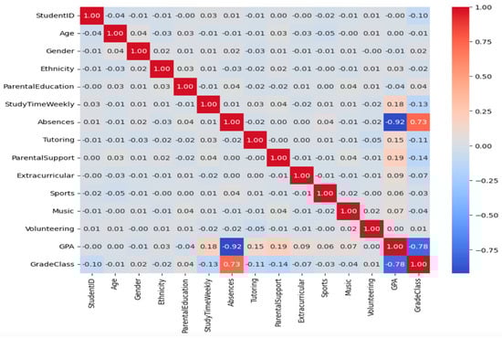
Figure 1.
Correlation matrix heat map.
Figure 1 shows that the academic achievement of the students decreases significantly as the number of absences increases. The data also show that students’ grade levels and academic achievement largely overlap. In addition, weak but positive relationships were found between some variables, such as parental support and tutoring and GPA. On the other hand, variables such as age, gender, ethnicity, and participation in music or sports activities have very low correlations with GPA. This suggests that these variables do not have a direct determining effect on academic achievement. In sum, this correlation analysis reveals that absences and grade level are most strongly associated with students’ academic achievement.
The data set comprises various academic and social variables associated with 2392 students. As shown in Table 1, the average number of absences is 14.54, with total absence duration ranging from 0 to 29 days, and a high standard deviation of 8.47. This situation reveals significant differences among students, in terms of absences. The parental support variable was coded between 1 and 4 and resulted in a mean of 2.12; most students received moderate support. The average weekly study time was 9.77 h, but this time shows a wide distribution, ranging between 0.001 and 19.97 h. Only 30 percent of the students took private lessons, and 38 percent participated in social activities. GPA, which represents academic performance, has a mean of 1.91 out of 4.00, with 50% of students scoring between 1.17 and 2.62. These results indicate significant differences among students in factors such as academic achievement, study time, parental support, and social activity participation, and that the effects of these variables on achievement are worth analyzing.

Table 1.
Statistics associated with data elements highly correlated with GPA.
Figure 2 illustrates the relationships between GPA and the four variables with the highest correlation coefficients: absences, grade class, parental support, and weekly study time. A strong negative correlation is observed between GPA and absences, suggesting that increased absenteeism reduces academic performance. Conversely, both weekly study time and parental support exhibit positive associations with GPA. These visualizations align with numerical correlation analysis and provide valuable insights into the impacts of these variables on students’ academic success.
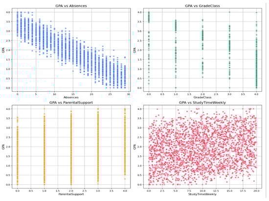
Figure 2.
Scatter plots of GPA versus the top four most-correlated features: absences, grade class, parental support, and weekly study time.
4. Model Training and Evaluation Methods
The data set used in the modeling process of this study was divided into two parts: training (80%) and testing (20%). The dependent variable was (GPA), and grade class and student ID variables were removed from the analysis during the modeling process. As independent variables, all other self-attributes were included in the model, as they were thought to affect students’ academic achievement.
The Python programming language was used in data processing, and the processes were conducted in a Spyder Enterger Development Environment. In this study, the Pandas, Numpy, Scikit-learn, Seaborn, Mathplotlib, and DEAP libraries were used for both the data preprocessing and modeling processes.
In this study, ten different regression models, namely, K-NNs, SVR, DT, RF, AdaBoost, ETR, GBM, BR, HGBR, and XGBoost, were applied to predict students’ academic achievement. Moreover, determination coefficient, mean absolute error, mean squared error, root mean squared error, mean squared error, mean squared log error, maximum error, explained variance, and ten additional metrics results were obtained for each model. The determination of the optimum hyperparameters of the models was performed using the genetic algorithm and grid search.
In the following subsections, firstly, the model performance measures are calculated, and then the hyperparameter optimization is performed.
4.1. Evaluation Metrics
Determining the appropriate metrics is an important step in evaluating the performance of machine learning models, measuring the accuracy of the models, and comparing different algorithms. In this study, the coefficient of determination (R2), mean absolute error (MAE), mean squared error (MSE), root mean squared error (RMSE), root mean squared error (RMSE), mean log squared error (MSLE), maximum error (MaxEr), and explained variance (ExVar) evaluation metrics, in addition to ten additional metrics, were used to compare predicted student achievement with actual values and analyze the effectiveness of the models. These metrics will be described in Table 2.
Table 2.
Statistical metrics [10].
In this table, is the actual value of the i-th sample, is the i-th value predicted by the model, is the mean of the actual values, is the arithmetic mean value, and n is the total number of observations.
The R2 value is a measure of how much of the total variance in the dependent variable (GPA) the model can explain. A high R2 value indicates that the model can provide a better explanation of the information associated with the independent variables, while a low R2 value indicates that the predictive power of the model is weak [26].
The MAE value is the average of the absolute MAE values of the differences between the model’s predicted values and the actual values. A low value indicates that the model makes more accurate predictions. The absence of negative values makes the evaluation more understandable [27].
The MSE value is calculated by averaging the squares of the prediction errors. Due to the squaring process, it gives higher weight to large errors and therefore reveals large deviations more clearly [28].
The RMSE is calculated by taking the square root of the MSE, and it improves interpretability by converting the unit of error to the original data scale [29].
The MSLE is the mean of the squares of the differences between the logarithmic transformations of the true and predicted values. It is especially used with positively skewed data, in cases in which the target variable has a wide range of values [30].
The MaxEr is the maximum value of the absolute differences between actual values and predicted values. This metric is used when it is important that the model does not make even a single prediction that is too inaccurate. It allows evaluation of worst-case performance, which is especially valuable in critical applications [31].
The ExVar is the proportion of variance between the model’s predictions and the actual values. This metric measures the proportion of variance explained by the model, with values closer to 1 indicating better model performance [23].
The MedAE shows the median value of the absolute errors between the predicted values and the actual values [29].
The MARE is the absolute difference between the actual and forecast values, divided by the actual values [32].
The MSRE is calculated as the mean of the squares of the relative differences between the actual and the predicted values [33].
The RMSRE is the square root of the MSRE, and provides a determination of the relative errors of the forecasts, converted to their original scale [30].
The RRMSE is the RMSE value divided by the mean of the data, and provides an assessment of the error measure relative to the size of the data [28].
The MBE is used to determine the bias of the model by measuring the average deviation associated with the predicted values [27].
The eMAX value shows the maximum value of all relative errors [34].
Standard deviation is a measure of dispersion that expresses the extent to which observations in a data set deviate from the arithmetic mean [35].
The t-statistic is a test statistic used to assess whether the difference between two sample means is statistically significant [36].
The 95% uncertainty interval shows the range in which the estimated values occur proximate to the true values with a 95% confidence level [37].
The evaluation metrics results of the models without hyperparameter optimization are given in Table 3.
Table 3.
Metric results of the ML models, without hyperparameter optimization.
In Table 3, it can be seen that SVR achieved the highest R2 = 0.95 and the lowest MSE = 0.04 and RMSE = 0.20, indicating that it successfully explained 95% of the variance in the data set and minimized the prediction errors.
GBM (R2 = 0.94, MSE = 0.05, and RMSE = 0.23) and HGBR (R2 = 0.94, MSE = 0.05, and RMSE = 0.22), closely followed SVR, offering high explanatory power and low mean-error performance. DT (R2 = 0.87, MSE = 0.11) and K-NNs (R2 = 0.9, MSE = 0.08) have a more limited explanatory power and relatively higher error values.
The SVR model achieved the best result for MAE, with MAE = 0.16, while the GBM also performed well, with MAE = 0.18, as did the HGBR model, with MAE = 0.17. The lowest MSLE was observed in the SVR model, with a value of 0.007, and in the GBM model, with a value of 0.01. The DT model showed the poorest performance, with the highest MSLE value, 0.02. The SVR model showed that it is the most robust model against outliers in its predictions, with the lowest worst-case deviation, MaxEr = 0.97, and eMAX = 30.02. In contrast, K-NNs, with eMAX = 81.53, and AdaBoost, with eMAX = 58.47, have high worst-case errors. The MARE, MSRE, RMSRE, and RRMSE metrics also showed that the SVR and GBM duo produced lower relative deviations, compared to the other models.
MBE remained around zero in all models, indicating no systematic bias; the smallest bias was observed in the GBM and ETR models. U95 had the narrowest confidence interval, with a value of 0.02 in the SVR and GBM models, and the widest confidence interval, with a value of 0.03 in the DT model. The analysis of the t-stat reveals that SVR and GBM do not show statistically significant bias, while the K-NNs and DT models may have more variable errors.
4.2. Hyperparameter Optimization with GA
In this section hyperparameter optimization using the GA will be performed for each ML model. In this study, the mutation rate, which is the probability of random changes in the genes of individuals, will be defined as 0.05, which means that 5% of individuals can change their parameters randomly. Also, the elitism rate is defined as 0.1, which means that 10% of the best individuals will be passed on to the next generation.
The default parameters of all ML models that we will use in this section are given in Table 4.
Table 4.
Default parameters of the ML models.
When determining the hyperparameter ranges for the GA and grid search methods, a balanced approach was adopted to ensure adequate representation of the search space while keeping the computational cost reasonable. Instead of trying 800 combinations in K-NNs, hyperparameter optimization was performed with GA by taking the population number as 20 and the gene number as 10; 200 combinations were completed, and a 75% screening saving was achieved by this combination. In the AdaBoost model, instead of scanning 600 combinations, hyperparameter optimization was applied with GA by taking the population number as 20 and the gene number as 10; 150 combinations were tried, and a 75% screening saving was achieved by the combination. While a total of 4000 combinations were to be scanned in all other algorithms, hyperparameter optimization was applied with GA by taking the population number as 100 and the gene number as 10, and a 75% screening saving was achieved by scanning the 1000 combinations. The aim of this strategy is to increase the applicability of the methods by preserving the representativeness of the search space and to provide a consistent basis for comparative analysis. Some of these calculations are described in the following:
GA-based hyperparameter optimization in the DT model started by restricting the search space to four different criteria values: squared_error, friedman_mse, absolute_error and poisson. The depth parameter was defined in ten equal steps in the range max_depth [1, 10], while the number of leaf nodes was divided into ten equal parts in the range max_leaf_nodes [2, 500]. Furthermore, the min_samples_leaf parameter, which determines the minimum number of samples that can be found in each leaf, is set to consist of ten possible values ranging from 1 to 10. This configuration enabled the GA to simultaneously search for both continuous variables in numerical ranges and categorical criteria with a limited number of options, and to perform an efficient search process within the defined population size and number of generations, instead of 4 × 10 × 10 × 10 = 4000 theoretical combinations in total, which can be seen in Table 4. Using hyperparameter optimization with GA, the population size was started at 100 individuals and the optimization process was carried out for 10 generations, resulting in a total of 1000 evaluated combinations. Although the total theoretical number of combinations was 4000, with the GA, instead of 4000 combinations, a total of 1000 individuals were evaluated, calculated as the sum of the product of the initial population, the number of generations and the population size. The best-performing combination identified by the GA was [criterion = absolute_error, max_depth = 10, max_leaf_nodes = 362, min_samples_leaf = 7].
The hyperparameter optimization of the RF model with the GA was designed to simultaneously explore a total of four different parameter sets. The n_estimators value, which determines the number of trees, was defined as starting from 100 and increasing in increments of 10 up to 1000; the criterion parameter was defined as a decision-tree splitting criterion with four possible values: squared_error, friedman_mse, absolute_error, and poisson. The max_depth parameter was set to have ten different values between 5 and 50, each in increments of five units (5, 10, ..., 50). Finally, the min_samples_leaf parameter was defined as containing ten equal values from 1 to 10. This configuration, according to Table 4 while theoretically defining 10 × 4 × 10 × 10 = 4000 possible combinations, allowed the GA to explore the entire solution space in an efficient evolutionary search process within the constraints of population and number of generations. Similar to the DT model, a total of 1000 individuals were evaluated by GA in the RF model. The best-performing combination identified by the GA was [n_estimators = 600, criterion = squared_error, max_depth = 95, min_samples_leaf = 2].
GA-based hyperparameter optimization in the K-NNs model is structured to cover four basic parameter sets. The n_neighbors is defined as containing ten different neighbor counts, namely, 3, 5, 7, 9, 11, 13, 15, 17, 19, and 21; weights is defined as containing two weighting strategies, uniform and distance; metric is defined as containing four distance metrics, namely, Minkowski, Euclidean, Manhattan, and Chebyshev; and leaf_size is defined as containing ten different values, starting from 10 and increasing by increments of 10 up to 100. This configuration yielded a total of 10 × 2 × 4 = 800 theoretical combinations, as shown in Table 4. However, the GA efficiently explored the search space by setting the population size to 20 individuals and the number of generations to 10, performing only 200 evaluations. The best performance was obtained with [n_neighbors = 15, weights = ‘distance’, metric = ‘manhattan’, leaf_size = 10].
In the AdaBoost model, GA-based hyperparameter optimization is structured to examine three basic parameter sets simultaneously. The n_estimators value is defined as starting from 100, increasing by increments of 100, and ranging up to 2000 (20 different values), while learning_rate, which controls the learning rate, is defined as ten equal increments from 0.01 to 1.0 (10 different values). Furthermore, the loss function, which determines the error weighting strategy of weak learners, was associated with three possible values, namely, linear, square, and exponential. This arrangement theoretically creates 600 different combinations, whereas GA only creates 150 different combinations within the framework of a population size of 15 individuals and 10 generations; 150 evaluations were performed to ensure an effective evolutionary filtering of the search space.
Similar to the above four ML models for which hyperparameter optimization was performed with the GA, the selected hyperparameters and their values for the six ML models are given in detail in Table 5.
Table 5.
Hyperparameters selected in the GA optimization process.
The evaluation metrics results of the models after hyperparameter optimization with GA are given in Table 6.
Table 6.
Metrics results of the ML models, with hyperparameters selected by GA.
In this comparative analysis, the XGBoost and GBM models achieved the highest scores for coefficient of determination, with R2 = 0.9449 and R2 = 0.9440, respectively, indicating that the two models each have a strong generalization ability. These models also excelled at the mean squared error level, achieving the lowest MSE (0.0455 and 0.0462) and RMSE (0.2134 and 0.2151).
SVR achieved the lowest mean absolute error, with MAE = 0.1827, closely followed by the XGBoost model, with MAE = 0.1660, and the GBM model, with MAE = 0.1680. In contrast, the BR model showed the lowest accuracy value, with R2 = 0.1082, well behind the other models. Moreover, the BR model exhibited significantly poor prediction performance, with the highest relevant values, namely, MSE = 0.7374, RMSE = 0.8587, and MAE = 0.7210.
The lowest values in terms of MSLE and MedAE were obtained by XGBoost and SVR. In the MaxEr and erMAX metrics, which are critical in terms of sensitivity to outlier predictions, the most successful models were again GBM and XGBoost, while the weakest model was BR.
In terms of MARE, MSRE, RMSRE, and RRMSE metrics, XGBoost and GBM provided consistent forecasts with the lowest bias values, while the BR and HGBR models provided less reliable forecasts.
The MBE metrics are close to zero in all models, indicating that the forecasts are free of systematic bias. However, a slight negative bias was observed in the K-NNs model, with MBE = −0.0249. The t-stat metric indicates non-significant biases in the SVR, GBM, and XGBoost models, while larger values were observed in the K-NNs and BR models, indicating that the forecasts are less stable.
According to the U95 metrics, the XGBoost model has a value of 0.0191 and the GBM model has a value of 0.0192. The results for these models show that their forecasts are not only accurate but also highly reliable.
4.3. Determination of Optimum Hyperparameters of Models with Grid Search
Another method used to improve model performance is grid search. Grid search aims to select the optimal combination according to the evaluation metric by performing a systematic search in the ranges of the hyperparameters defined for each model. During the optimization process, the performance of each model was evaluated via cross-validation, and the hyperparameters with the lowest error values were determined. The hyperparameters selected by the grid search method can be seen in Table 7.
Table 7.
The hyperparameters selected by the grid search method.
The evaluation metrics results of the models after hyperparameter optimization with the grid search method are given in Table 8.
Table 8.
Metrics results of the ML models, with hyperparameters selected by the grid search method.
According to the metric results obtained after hyperparameter estimation using the grid search method, the models with the highest R2 values are the SVR, XGBoost, and GBM models, with values of 0.9519, 0.9474, and 0.9469, respectively. These models successfully explained most of the variance in the data set. The lowest R2 value was observed in the Bagging Regressor model, with a value of 0.1432, indicating that the model had difficulty in capturing the patterns in the data.
The lowest MSE and RMSE values belong to the SVR (0.0398, 0.1994), XGBoost (0.0435, 0.2085) and GBM (0.0438, 0.2094) models respectively. This suggests that these models work with both small errors and consistent forecasts. The highest error values were again observed in the BR model (MSE = 0.7085, RMSE = 0.8417), indicating that the generalization capacity of the model is weak.
In terms of MAE, the SVR (0.1594), XGBoost (0.1638), and GBM (0.1645) models again stood out, while the BR model (0.7067) exhibited low accuracy with high bias. A similar ranking was observed in terms of MSLE and MedAE metrics, with the XGBoost and SVR models dominating as to the MSLE and MedAE values.
MaxEr and erMAX were the highest in the BR model, at 1.998 and 176.93, respectively, indicating that the model is highly sensitive to extreme values. In contrast, SVR and XGBoost provided more stable forecasts with relatively low values in these metrics.
When the MARE, MSRE, RMSRE, and RRMSE results are analyzed, it can be understood that the SVR, XGBoost and GBM models offer more robust and balanced forecasting performance with low rates of error. The BR model showed significant relative bias, especially in the MSRE (142.01) and RMSRE (11.92) values.
The MBE values are close to zero for all models, indicating that the forecasts are free of systematic bias. In terms of SD and t-stat, the SVR and XGBoost models stand out, which supports the consistency and statistical significance associated with their forecasts. In particular, the SVR model has a low confidence interval and low statistical stability, with t-stat = 0.402 and U95 = 0.0179.
5. Discussion and Conclusions
In this study, ten different regression models, namely, the K-NNs, SV, DT, RF, AdaBoost, ETR, GBM, BR, HBGR, and XGBoost methods for predicting student academic achievement are compared, and their performances are improved via hyperparameter optimization. In this study, generalization capabilities were evaluated using 10-fold cross-validation in the modeling process, and model performances were analyzed through seventeen statistical metrics, namely, R2, MAE, MSE, RMSE, MSLE, MaxEr, ExVar, MedAE, MARE, MSRE, RMSRE, RRMSE, MBE, eMAX, SD, t-stat, and U95.
Firstly, our ML models are evaluated, using the seventeen metrics given above, without hyperparameter optimization. According to this analysis, the SVR model, which combines the highest explanatory power and the lowest error level, successfully explained 95% of the variance in the data set, with R2 = 0.95, MSE = 0.04, RMSE = 0.20, and MAE = 0.16, demonstrating the best performance in terms of both generalization capacity and prediction accuracy. The GBM and HGBR models follow the SVR model, with R2 = 0.94 and MAE = 0.18, respectively. On the other hand, the single-tree-based DT and K-NNs methods lagged behind with significantly higher error rates.
Afterwards, our ML models underwent hyperparameter optimization with GA and were evaluated with the seventeen metrics. Given the results, the XGBoost and GBM models stand out as the strongest models in terms of both error metrics and explanatory power, and SVR stands out as having low absolute errors, while the BR and HGBR models perform more poorly in terms of both error levels and reliability. These findings clearly indicate that ensemble methods should be preferred in applications requiring high accuracy.
Finally, the grid search method is used for hyperparameter optimization in our ML models. According to the results, the SVR, XGBoost, and GBM models stand out in terms of overall error and explanatory performance, whereas the BR model is weak in both absolute and relative error rates and is therefore considered to be a model that should not be preferred in this data set. Considering both performance and computational cost in model selection, it is recommended that balanced models such as SVR and GBM should be prioritized.
In conclusion, despite the different hyperparameter optimization strategies applied in this study, certain machine learning models generally exhibited consistent and superior performance. In particular, the SVR, GBM, and XGBoost models stand out as models with both high explanatory power and low error rates in such metrics as MSE, RMSE, and MAE. This finding indicates that these models should be prioritized in regression problems requiring high accuracy. On the other hand, the BR and (partially) HGBR models produced poor results in both absolute and relative error metrics; therefore, it is understood that success is not guaranteed even if an ensemble method is applied in such data structures. In this context, the interaction of each model with the data set should be contextualized. Consequently, the multi-stage evaluation reveals that ensemble methods, especially GBM and XGBoost, together with kernel-based methods such as SVR, which can model complex nonlinear structures, offer more stable performances, compared to other models in terms of both generalization ability and fault tolerance. Moreover, considering the sensitivity of these models to hyperparameter optimization, it is recommended to prefer balanced models such as SVR and GBM when considering the trade-off between performance and computational cost.
The data set used in this study includes specific characteristics that are thought to affect students’ academic achievement. In future studies, including different variables such as student motivation, teacher feedback, learning environment, etc., in the model might enhance performance. In addition, the contribution of different machine learning techniques, such as deep learning and support vector machines in the prediction of student achievement can also be examined.
In addition, only the genetic algorithm and grid search were used in the optimization process. In future studies, other hyperparameter optimization methods, such as Bayesian Optimization or Random Search, can be evaluated and performance comparisons made. Finally, the generalizability of the proposed models can be tested by conducting studies on data sets from different training systems.
Author Contributions
Conceptualization, B.D. and T.H.; methodology, B.D.; software, T.H.; validation, B.D. and T.H.; formal analysis, B.D.; investigation, T.H.; resources, B.D. and T.H.; data curation, T.H.; writing—original draft preparation, T.H.; writing—review and editing, B.D.; visualization, T.H.; supervision, B.D. All authors have read and agreed to the published version of the manuscript.
Funding
This research received no external funding.
Data Availability Statement
The data presented in this study are openly available in [https://www.kaggle.com/datasets/tusharika802/student-performance-data-csv, accessed on 19 May 2025].
Acknowledgments
The authors would like to thank Onur Uğurlu for his guidance regarding this study. They would also like to thank the referees and editors for their valuable support.
Conflicts of Interest
The authors declare no conflicts of interest.
References
- Yağcı, M. Educational data mining: Prediction of students’ academic performance using machine learning algorithms. Smart Learn. Environ. 2022, 9, 11. [Google Scholar] [CrossRef]
- Ting, T.T.; Loh, E.S.; Koong, J.L.; Tham, H.H.; Salau, A.O. Prediction of student academic status in higher education through machine learning. Pak. J. Life Soc. Sci. 2024, 22, 19224–19238. [Google Scholar]
- Villar, A.; Andrade, C.R.V. Supervised machine learning algorithms for predicting student dropout and academic success: A comparative study. Discov. Artif. Intell. 2024, 4, 2. [Google Scholar] [CrossRef]
- Alkan, A. Öğrencilerin sınavlardaki performansının makine öğrenmesi teknikleriyle tahminlenmesi. Osman. Korkut Ata Univ. J. Inst. Sci. 2024, 7, 1116–1128. [Google Scholar] [CrossRef]
- Bayırbağ, V.; Bakır, H. Çalışan Yıpranması Tahmin Etmek için Hiper Parametresi Ayarlanmış Makine Öğrenme Algoritmaların Kullanılması. In Proceedings of the International Conference on Scientific and Academic Research, Konya, Turkey, 2–4 June 2023; Volume 1, pp. 466–471. [Google Scholar]
- Khan, M.A.; Zafar, A.; Farooq, F.; Javed, M.F.; Alyousef, R.; Alabduljabbar, H.; Khan, M.I. Geopolymer concrete compressive strength via artificial neural network, adaptive neuro-fuzzy interface system, and gene expression programming with K-fold cross validation. Front. Mater. 2021, 8, 621163. [Google Scholar] [CrossRef]
- Yang, L.; Shami, A. On hyperparameter optimization of machine learning algorithms: Theory and practice. Neurocomputing 2020, 415, 295–316. [Google Scholar] [CrossRef]
- Arévalo-Cordovilla, F.E.; Peña, M. Comparative Analysis of Machine Learning Models for Predicting Student Success in Online Programming Courses: A Study Based on LMS Data and External Factors. Mathematics 2024, 12, 3272. [Google Scholar] [CrossRef]
- Zou, W.; Zhong, W.; Du, J.; Yuan, L. Prediction of Student Academic Performance Utilizing a Multi-Model Fusion Approach in the Realm of Machine Learning. Appl. Sci. 2025, 15, 3550. [Google Scholar] [CrossRef]
- Asgarkhani, N.; Kazemi, F.; Jankowski, R. Machine learning-based prediction of residual drift and seismic risk assessment of steel moment-resisting frames considering soil-structure interaction. Comput. Struct. 2023, 289, 107181. [Google Scholar] [CrossRef]
- Wang, X.; Mei, X.; Huang, Q.; Han, Z.; Huang, C. Fine-grained learning performance prediction via adaptive sparse self-attention networks. Inf. Sci. 2021, 545, 223–240. [Google Scholar] [CrossRef]
- Huang, Q.; Chen, J. Enhancing academic performance prediction with temporal graph networks for massive open online courses. J. Big Data 2024, 11, 52. [Google Scholar] [CrossRef]
- Huang, Q.; Zeng, Y. Improving academic performance predictions with dual graph neural networks. Complex Intell. Syst. 2024, 10, 3557–3575. [Google Scholar] [CrossRef]
- Wang, X.; Wu, P.; Liu, G.; Huang, Q.; Hu, X.; Xu, H. Learning performance prediction via convolutional GRU and explainable neural networks in e-learning environments. Computing 2019, 101, 587–604. [Google Scholar] [CrossRef]
- Cover, T.M.; Hart, P.E. Nearest neighbor pattern classification. IEEE Trans. Inf. Theory 1967, 13, 21–27. [Google Scholar] [CrossRef]
- Drucker, H.; Burges, C.J.C.; Kaufman, L.; Smola, A.; Vapnik, V. Support vector regression machines. In Advances in Neural Information Processing Systems; MIT Press: Cambridge, MA, USA, 1997; Volume 9, pp. 155–161. [Google Scholar]
- Quinlan, J.R. Induction of decision trees. Mach. Learn. 1986, 1, 81–106. [Google Scholar] [CrossRef]
- Breiman, L. Random forests. Mach. Learn. 2001, 45, 5–32. [Google Scholar] [CrossRef]
- Geron, A. Scikit-Learn, Keras ve TensorFlow ile Uygulamalı Makine Öğrenmesi, 1st ed.; Aksoy, B.; Kaya, Ö., Translators; Buzdağı Yayınevi: Ankara, Turkey, 2021. [Google Scholar]
- Friedman, J.H. Greedy function approximation: A gradient boosting machine. Ann. Stat. 2001, 29, 1189–1232. [Google Scholar] [CrossRef]
- Geurts, P.; Ernst, D.; Wehenkel, L. Extremely randomized trees. Mach. Learn. 2006, 63, 3–42. [Google Scholar] [CrossRef]
- Breiman, L. Bagging predictors. Mach. Learn. 1996, 24, 123–140. [Google Scholar] [CrossRef]
- Pedregosa, F.; Varoquaux, G.; Gramfort, A.; Michel, V.; Thirion, B.; Grisel, O.; Blondel, M.; Prettenhofer, P.; Weiss, R.; Dubourg, V.; et al. Scikit-learn: Machine learning in Python. J. Mach. Learn. Res. 2011, 12, 2825–2830. [Google Scholar]
- Chen, T.; Guestrin, C. XGBoost: A scalable tree boosting system. In Proceedings of the 22nd ACM SIGKDD International Conference on Knowledge Discovery and Data Mining, San Francisco, CA, USA, 13–17 August 2016; pp. 785–794. [Google Scholar]
- Available online: https://www.kaggle.com/datasets/tusharika802/student-performance-data-csv (accessed on 19 August 2024).
- James, G.; Witten, D.; Hastie, T.; Tibshirani, R. An Introduction to Statistical Learning: With Applications in R; Springer: New York, NY, USA, 2013. [Google Scholar]
- Willmott, C.J.; Matsuura, K. Advantages of the mean absolute error (MAE) over the root mean square error (RMSE). Clim. Res. 2005, 30, 79–82. [Google Scholar] [CrossRef]
- Hyndman, R.J.; Koehler, A.B. Another look at measures of forecast accuracy. Int. J. Forecast. 2006, 22, 679–688. [Google Scholar] [CrossRef]
- Chai, T.; Draxler, R.R. Root mean square error (RMSE) or mean absolute error (MAE)? Geosci. Model Dev. 2014, 7, 1247–1250. [Google Scholar] [CrossRef]
- Botchkarev, A. Performance metrics (error measures) in machine learning regression, forecasting and prognostics: Properties and typology. arXiv 2018, arXiv:1809.03006. [Google Scholar]
- Shcherbakov, M.V.; Brebels, A.; Shcherbakova, N.L.; Tyukov, A.P.; Janovsky, T.A.; Kamaev, V.A. A survey of forecast error measures. World Appl. Sci. J. 2013, 24, 171–176. [Google Scholar]
- Armstrong, J.S.; Collopy, F. Error measures for generalizing about forecasting methods: Empirical comparisons. Int. J. Forecast. 1992, 8, 69–80. [Google Scholar] [CrossRef]
- Makridakis, S.; Andersen, A.; Carbone, R.; Fildes, R.; Hibon, M.; Lewandowski, R.; Winkler, R. The accuracy of extrapolation (time series) methods: Results of a forecasting competition. J. Forecast. 1982, 1, 111–153. [Google Scholar] [CrossRef]
- Tofallis, C. A better measure of relative prediction accuracy for model selection and model estimation. J. Oper. Res. Soc. 2015, 66, 1352–1362. [Google Scholar] [CrossRef]
- Montgomery, D.C.; Runger, G.C. Applied Statistics and Probability for Engineers, 7th ed.; Wiley: Hoboken, NJ, USA, 2018. [Google Scholar]
- Kutner, M.H.; Nachtsheim, C.J.; Neter, J.; Li, W. Applied Linear Statistical Models, 5th ed.; McGraw-Hill: Boston, MA, USA, 2005. [Google Scholar]
- Coleman, H.W.; Steele, W.G. Experimentation, Validation, and Uncertainty Analysis for Engineers, 4th ed.; Wiley: Hoboken, NJ, USA, 2018. [Google Scholar]
Disclaimer/Publisher’s Note: The statements, opinions and data contained in all publications are solely those of the individual author(s) and contributor(s) and not of MDPI and/or the editor(s). MDPI and/or the editor(s) disclaim responsibility for any injury to people or property resulting from any ideas, methods, instructions or products referred to in the content. |
© 2025 by the authors. Licensee MDPI, Basel, Switzerland. This article is an open access article distributed under the terms and conditions of the Creative Commons Attribution (CC BY) license (https://creativecommons.org/licenses/by/4.0/).