
Explainable Two-Layer Mode Machine Learning Method for Hyperspectral Image Classification


Abstract
1. Introduction
2. Band Selection with Sparse Space Clustering
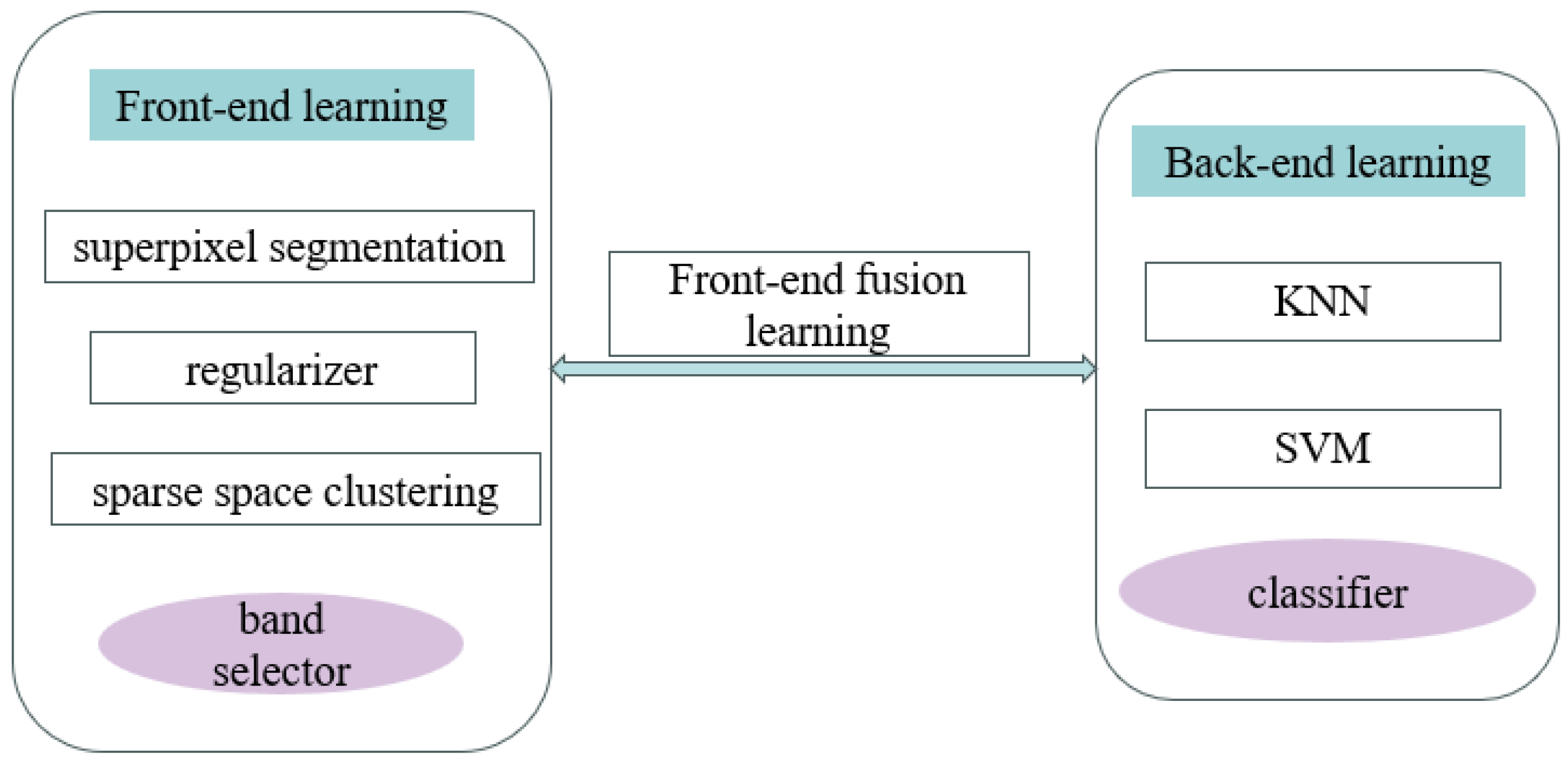
3. HSI Classification Method in Explainable Two-Layer Mode
3.1. Front-End Learning Layer for Data Re-Expression
3.1.1. Segment HSI with Superpixel Segmentation
3.1.2. Explainable Minimization Problem for SSC
3.2. Back-End Learning Layer for HSI Classification
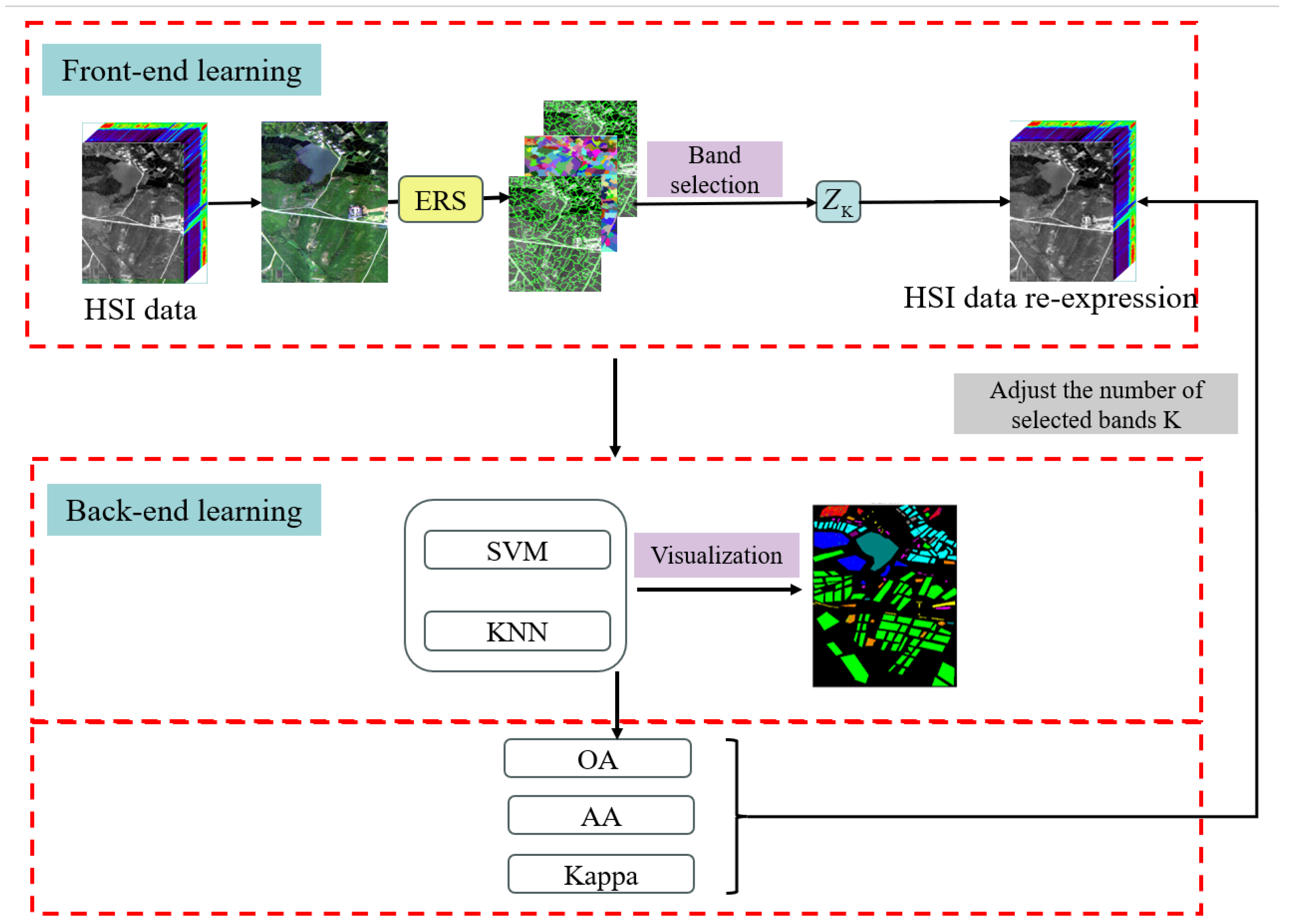
3.3. Two-Layer Mode HSI Classification Method
| Algorithm 1: Classification Algorithm under two-Layer Mode (CALM) |
| Input: HSI data |
| Output: The index set of the selected band ZK. |
| Step 1: Segment H into N regions with the index set s1, s2, ..., sN via ERS. |
| Step 2: Compute F with the index set S1, S2, ..., SN. |
| Step 3: Compute then goto Step 6, else, go to Step 4. |
| Step 4: Update Z with (5). |
| Step 5: Update S with (8), go to step 3. |
| Step 6: Let Z = (Z + ZT)/Z, and generate ZK with spectral clustering algorithm. |
| Step 7: Using ZK as input, train a classification model using SVM or KNN, andcalculate the evaluation metrics obtained by selecting K bands. |
| Step 8: |
4. Experiments
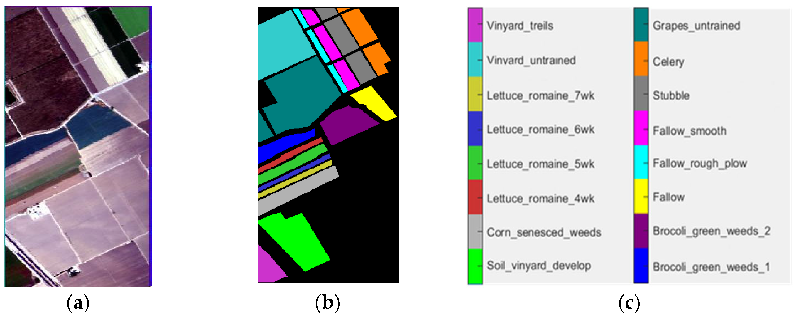
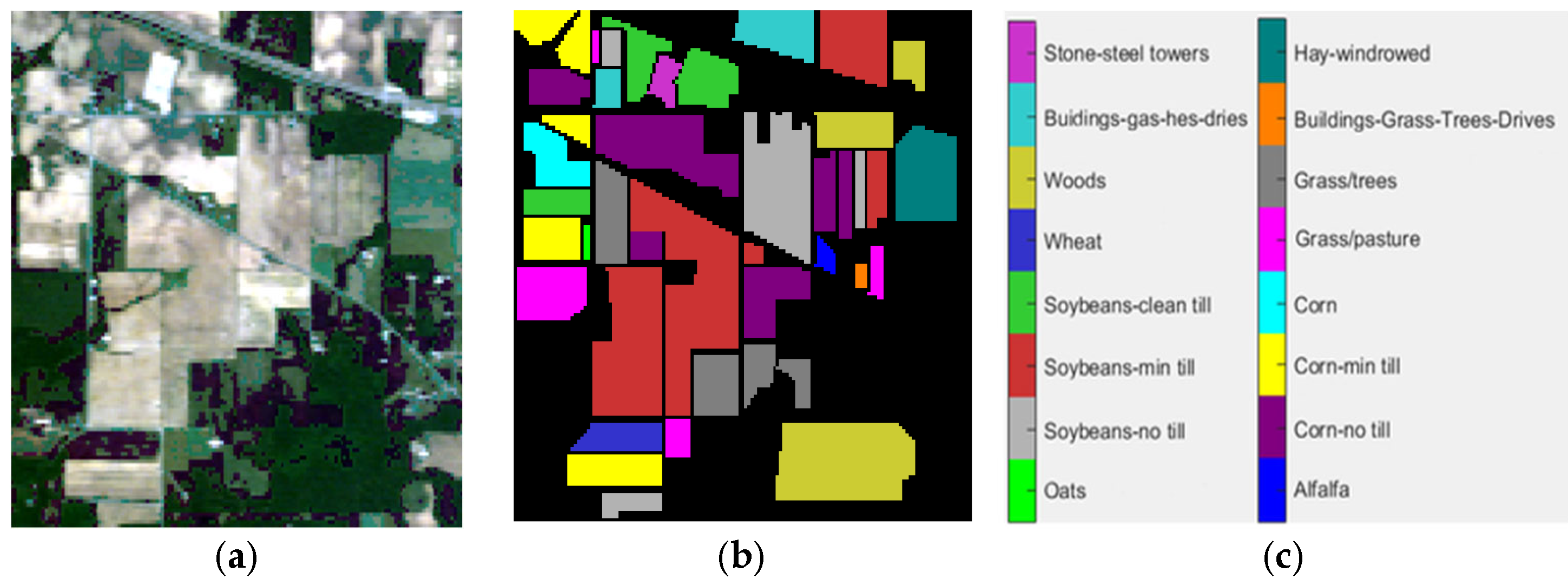
4.1. Datasets
4.2. Comparison Algorithms
4.3. Experimental Setup
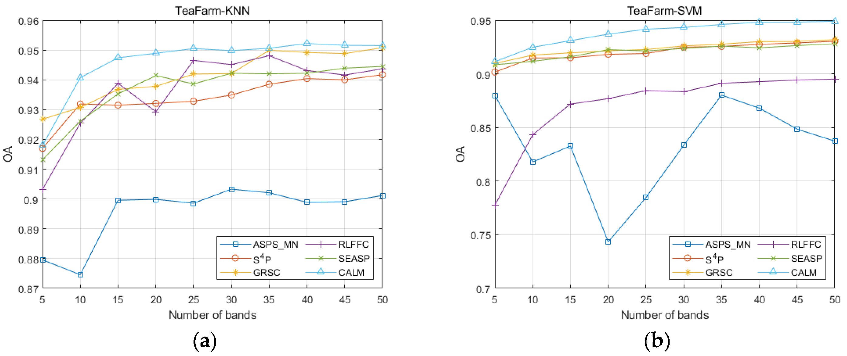
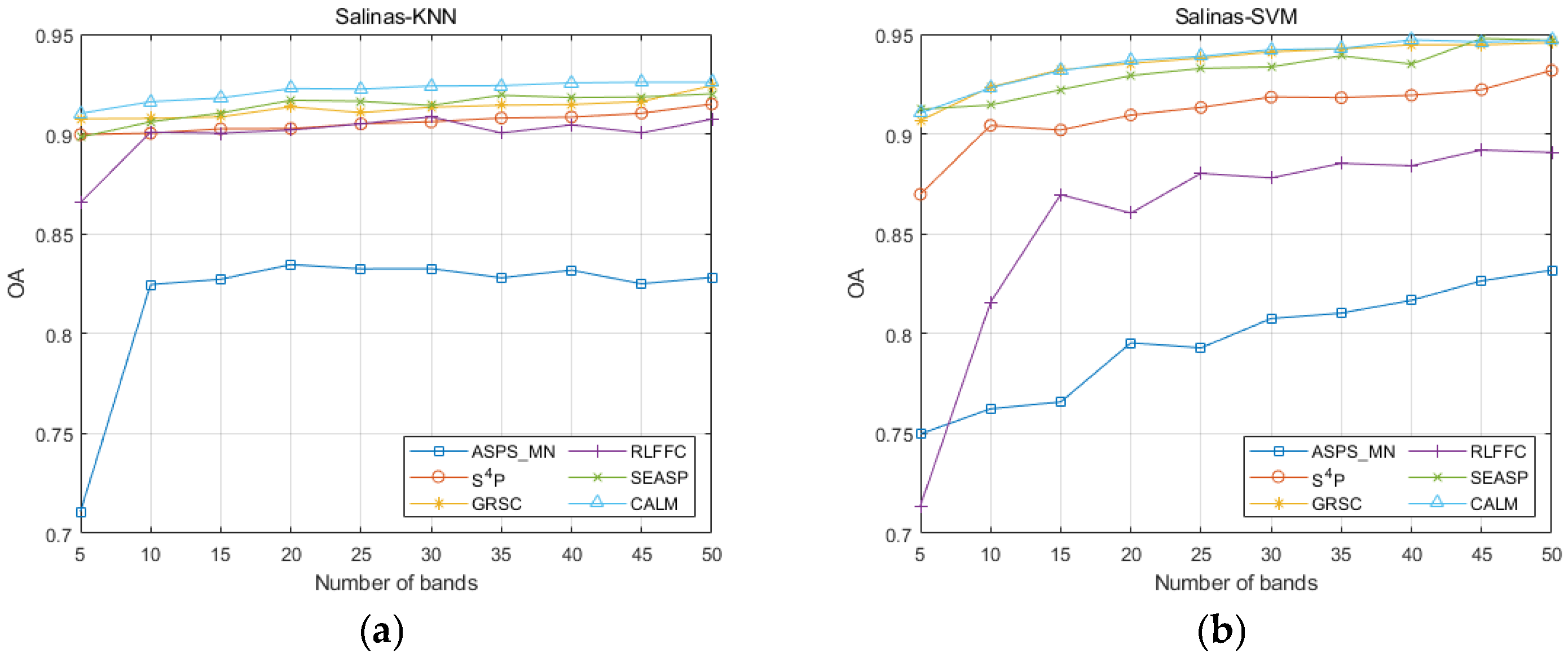
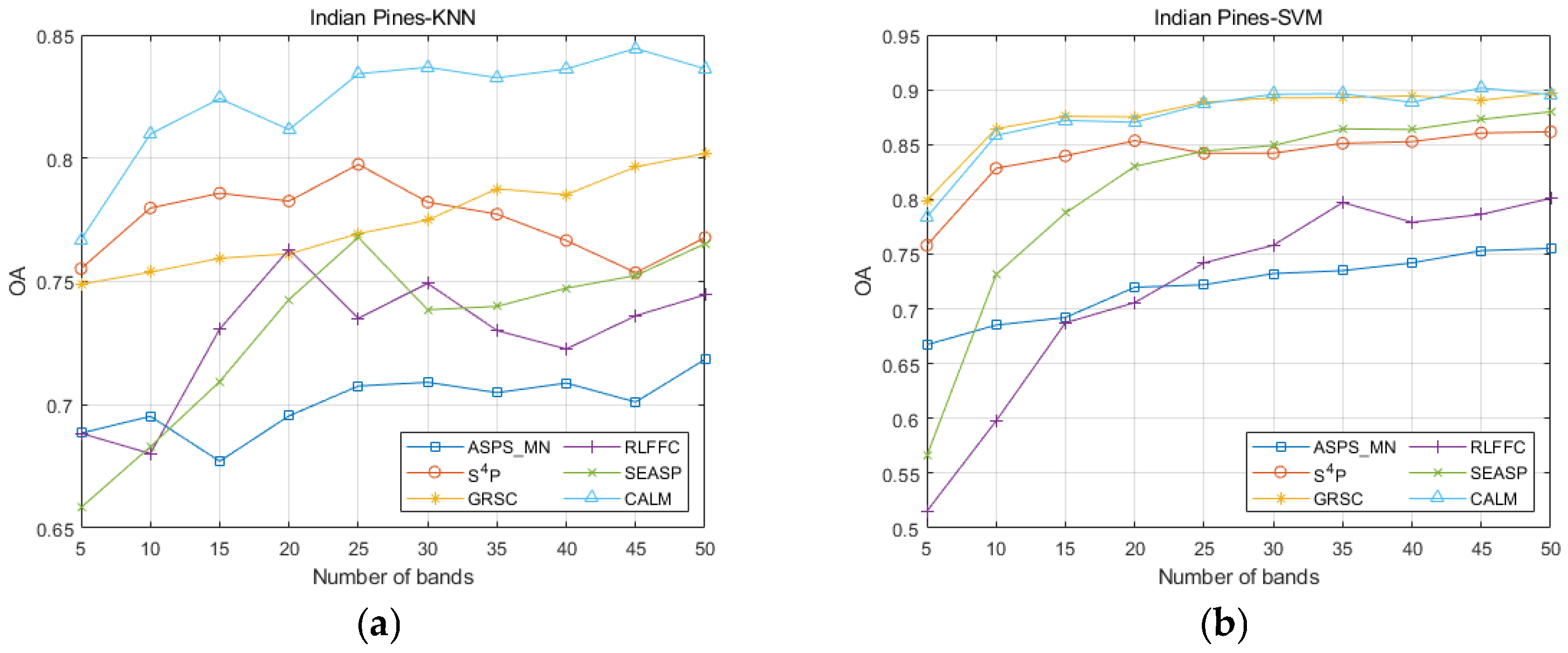
4.4. Experimental Results
5. Conclusions
Author Contributions
Funding
Institutional Review Board Statement
Informed Consent Statement
Data Availability Statement
Acknowledgments
Conflicts of Interest
References
- Cheng, M.-F.; Mukundan, A.; Karmakar, R.; Valappil, M.A.E.; Jouhar, J.; Wang, H.C. Modern Trends and Recent Applications of Hyperspectral Imaging: A Review. Technologies 2025, 13, 170. [Google Scholar] [CrossRef]
- Zhang, Y.; Wu, W.; Zhou, X.; Cheng, J.H. Non-Destructive Detection of Soybean Storage Quality Using Hyperspectral Imaging Technology. Molecules 2025, 30, 1357. [Google Scholar] [CrossRef]
- Zhang, Z.; Huang, L.; Wang, Q.; Jiang, L.; Qi, Y.; Wang, S.; Gu, Y. UAV Hyperspectral Remote Sensing Image Classification: A Systematic Review. IEEE J. Sel. Top. Appl. Earth Obs. Remote Sens. 2025, 18, 3099–3124. [Google Scholar] [CrossRef]
- Pushpalatha, V.; Mallikarjuna, P.B.; Mahendra, H.N.; Subramoniam, S.R.; Mallikarjunaswamy, S. Land use and land cover classification for change detection studies using convolutional neural network. Appl. Comput. Geosci. 2025, 25, 100227. [Google Scholar] [CrossRef]
- Valme, D.; Rassõlkin, A.; Liyanage, D.C. From ADAS to Material-Informed Inspection: Review of Hyperspectral Imaging Applications on Mobile Ground Robots. Sensor 2025, 25, 2346. [Google Scholar] [CrossRef]
- Ma, K.; Yao, C.; Liu, B.; Hu, Q.; Li, S.; He, P.; Han, J. Segment Anything Model-Based Hyperspectral Image Classification for Small Samples. Remote Sens. 2025, 17, 1349. [Google Scholar] [CrossRef]
- Hennessy, A.; Clarke, K.; Lewis, M. Hyperspectral Classification of Plants: A Review of Waveband Selection Generalisability. Remote Sens. 2020, 12, 113. [Google Scholar] [CrossRef]
- Mianji, F.A.; Zhang, Y. Robust hyperspectral classification using relevance vector machine. IEEE Trans. Geosci. Remote Sens. 2011, 49, 2100–2112. [Google Scholar] [CrossRef]
- Zhao, X.; Ma, J.; Wang, L.; Zhang, Z.; Ding, Y.; Xiao, X. A review of hyperspectral image classification based on graph neural networks. Artif. Intell. Rev. 2025, 58, 172. [Google Scholar] [CrossRef]
- He, Z.; Xia, K.; Zhang, J.; Wang, S.; Yin, Z. An enhanced semi-supervised support Vector Machine Algorithm for spectral-spatial hyperspectral image classification. Pattern Recognit. Image Anal. 2024, 34, 199–211. [Google Scholar]
- Chen, C.; Yuan, X.; Gan, S.; Kang, X.; Luo, W.; Li, R.; Gao, S. A new strategy based on multi-source remote sensing data for improving the accuracy of land use/cover change classification. Sci. Rep. 2024, 14, 26855. [Google Scholar] [CrossRef] [PubMed]
- Banerjee, A.; Swain, S.; Rout, M.; Bandyopadhyay, M. Composite spectral spatial pixel CNN for land-use hyperspectral image classification with hybrid activation function. Multimed. Tools Appl. 2024, 84, 10527–10550. [Google Scholar] [CrossRef]
- Liu, J.; Lan, J.; Zeng, Y.; Luo, W.; Zhuang, Z.; Zou, J. Explainability Feature Bands Adaptive Selection for Hyperspectral Image Classification. Remote Sens. 2025, 17, 1620. [Google Scholar] [CrossRef]
- Hassija, V.; Chamola, V.; Mahapatra, A.; Singal, A.; Goel, D.; Huang, K.; Hussain, A. Interpreting black-box models: A review on explainable artificial intelligence. Cogn. Comput. 2024, 16, 45–74. [Google Scholar] [CrossRef]
- Contreras, J.; Bocklitz, T. Explainable artificial intelligence for spectroscopy data: A review. Pflügers Arch. Eur. J. Physiol. 2024, 477, 603–615. [Google Scholar] [CrossRef]
- Li, R.; Zheng, S.; Duan, C.; Yang, Y.; Wang, X. Classification of hyperspectral image based on double-branch dual-attention mechanism network. Remote Sens. 2020, 12, 582. [Google Scholar] [CrossRef]
- Yu, H.; Zhang, H.; Liu, Y.; Zheng, K.; Xu, Z.; Xiao, C. Dual-channel convolution network with image-based global learning framework for hyperspectral image classification. IEEE Geosci. Remote Sens. Lett. 2021, 19, 1–5. [Google Scholar] [CrossRef]
- Li, T.; Zhang, X.; Zhang, S.; Wang, L. Self-supervised learning with a dual-branch ResNet for hyperspectral image classification. IEEE Geosci. Remote Sens. Lett. 2022, 19, 1–5. [Google Scholar] [CrossRef]
- Wang, C.; Zhan, C.; Lu, B.; Yang, W.; Zhang, Y.; Wang, G.; Zhao, Z. SSFAN: A Compact and Efficient Spectral-Spatial Feature Extraction and Attention-Based Neural Network for Hyperspectral Image Classification. Remote Sens. 2024, 16, 4202. [Google Scholar] [CrossRef]
- Tang, X.; Zhang, K.; Zhou, X.; Zeng, L.; Huang, S. Enhancing Binary Convolutional Neural Networks for Hyperspectral Image Classification. Remote Sens. 2024, 16, 4398. [Google Scholar] [CrossRef]
- Zhao, H.; Lu, Z.; Sun, S.; Wang, P.; Jia, T.; Xie, Y.; Xu, F. Classification of Large Scale Hyperspectral Remote Sensing Images Based on LS3EU-Net++. Remote Sens. 2025, 17, 872. [Google Scholar] [CrossRef]
- Wang, J.; Tang, C.; Zheng, X.; Liu, X.; Zhang, W.; Zhu, E. Graph regularized spatial–spectral subspace clustering for hyperspectral band selection. Neural Netw. 2022, 153, 292–302. [Google Scholar] [CrossRef]
- Wang, Y.; Ma, H.; Yang, Y.; Zhao, E.; Song, M.; Yu, C. Self-supervised deep multi-level representation learning fusion-based maximum entropy subspace clustering for hyperspectral band selection. Remote Sens. 2024, 16, 224. [Google Scholar] [CrossRef]
- Wang, Q.; Li, Q.; Li, X. A fast neighborhood grouping method for hyperspectral band selection. IEEE Trans. Geosci. Remote Sens. 2020, 59, 5028–5039. [Google Scholar] [CrossRef]
- Liu, K.; Chen, Y.; Chen, T. A band subset selection approach based on sparse self-representation and band grouping for hyperspectral image classification. Remote Sens. 2022, 14, 5686. [Google Scholar] [CrossRef]
- Zhao, H.; Bruzzone, L.; Guan, R.; Zhou, F.; Yang, C. Spectral-spatial genetic algorithm-based unsupervised band selection for hyperspectral image classification. IEEE Trans. Geosci. Remote Sens. 2021, 59, 9616–9632. [Google Scholar] [CrossRef]
- Habermann, M.; Fremont, V.; Shiguemori, E.H. Supervised band selection in hyperspectral images using single-layer neural networks. Int. J. Remote Sens. 2019, 40, 3900–3926. [Google Scholar] [CrossRef]
- Elhamifar, E.; Vidal, R. Sparse subspace clustering: Algorithm, theory, and applications. IEEE Trans. Pattern Anal. Mach. Intell. 2013, 35, 2765–2781. [Google Scholar] [CrossRef]
- Sun, W.; Zhang, L.; Du, B.; Li, W.; Lai, Y.M. Band selection using improved sparse subspace clustering for hyperspectral imagery classification. IEEE J. Sel. Top. Appl. Earth Obs. Remote Sens. 2015, 8, 2784–2797. [Google Scholar] [CrossRef]
- Ng, A.; Jordan, M.; Weiss, Y. On spectral clustering: Analysis and an algorithm. Adv. Neural Inf. Process. Syst. 2001, 14, 849–856. [Google Scholar]
- Guo, T.; Han, C.; Li, M. Fusion of front-end and back-end learning based on layer-by-layer data re-representation. Sci. Sin. Inform. 2019, 49, 739–759. (In Chinese) [Google Scholar] [CrossRef]
- Liu, M.; Tuzel, O.; Ramalingam, S.; Chellappa, R. Entropy rate superpixel segmentation. In Proceedings of the IEEE Conference on Computer Vision and Pattern Recognition (CVPR), Colorado Springs, CO, USA, 20–25 June 2011; pp. 2097–2104. [Google Scholar]
- Li, X.; Chen, J.; Zhao, L.; Li, H.; Wang, J.; Sun, L.; Guo, S.; Chen, P.; Zhao, X. Superpixel segmentation based on anisotropic diffusion model for object-oriented remote sensing image classification. IEEE J. Sel. Top. Appl. Earth Obs. Remote Sens. 2023, 17, 7621–7639. [Google Scholar] [CrossRef]
- Wang, Q.; Li, Q.; Li, X. Hyperspectral band selection via adaptive subspace partition strategy. IEEE J. Sel. Top. Appl. Earth Obs. Remote Sens. 2019, 12, 4940–4950. [Google Scholar] [CrossRef]
- Tang, C.; Wang, J. A hyperspectral band selection method via adjacent subspace partition. Tientsin Univ. J. 2022, 55, 255–262. [Google Scholar]
- Tang, C.; Wang, J.; Zheng, X.; Liu, X.; Xie, W.; Li, X.; Zhu, X. Spatial and spectral structure preserved self-representation for unsupervised hyperspectral band selection. IEEE Trans. Geosci. Remote Sens. 2023, 61, 1–13. [Google Scholar] [CrossRef]
- Wang, J.; Tang, C.; Li, Z.; Liu, X.; Zhang, W.; Zhu, E.; Wang, L. Hyperspectral band selection via region-aware latent features fusion based clustering. Inf. Fusion 2022, 79, 162–173. [Google Scholar] [CrossRef]
- Wang, H.; Yu, G.; Cheng, J.; Zhang, Z.; Wang, X.; Xu, Y. Fast hyperspectral image classification with strong noise robustness based on minimum noise fraction. Remote Sens. 2024, 16, 3782. [Google Scholar] [CrossRef]


| Datasets | Classifier | Metrics | ASPS_MN | S4P | GRSC | RLFFC | SEASP | CALM |
|---|---|---|---|---|---|---|---|---|
| TeaFarm | KNN | OA | 0.9012 | 0.9417 | 0.9508 | 0.9437 | 0.9445 | 0.9522 |
| AA | 0.7747 | 0.8576 | 0.8638 | 0.8633 | 0.8647 | 0.8902 | ||
| Kappa | 0.8932 | 0.9152 | 0.9140 | 0.9180 | 0.9194 | 0.9302 | ||
| SVM | OA | 0.8802 | 0.9304 | 0.9319 | 0.8951 | 0.9281 | 0.9490 | |
| AA | 0.7479 | 0.7491 | 0.7480 | 0.6 851 | 0.7397 | 0.8632 | ||
| Kappa | 0.6747 | 0.8987 | 0.9007 | 0.8472 | 0.8953 | 0.9255 | ||
| Salinas | KNN | OA | 0.8282 | 0.9150 | 0.9242 | 0.9074 | 0.9201 | 0.9260 |
| AA | 0.8830 | 0.9565 | 0.9629 | 0.9537 | 0.9610 | 0.9637 | ||
| Kappa | 0.8172 | 0.9075 | 0.9174 | 0.8994 | 0.9129 | 0.9193 | ||
| SVM | OA | 0.8318 | 0.9318 | 0.9458 | 0.8908 | 0.9478 | 0.9469 | |
| AA | 0.8849 | 0.9673 | 0.9738 | 0.9320 | 0.9721 | 0.9757 | ||
| Kappa | 0.8210 | 0.9255 | 0.9259 | 0.8812 | 0.9418 | 0.9417 | ||
| Indian Pines | KNN | OA | 0.7184 | 0.7678 | 0.8644 | 0.7446 | 0.7653 | 0.8363 |
| AA | 0.7324 | 0.7678 | 0.8000 | 0.6824 | 0.7150 | 0.8285 | ||
| Kappa | 0.6885 | 0.7479 | 0.7807 | 0.7234 | 0.7449 | 0.8285 | ||
| SVM | OA | 0.7552 | 0.8616 | 0.8971 | 0.8009 | 0.8799 | 0.9016 | |
| AA | 0.7284 | 0.8626 | 0.8976 | 0.7412 | 0.8852 | 0.8989 | ||
| Kappa | 0.7352 | 0.8477 | 0.8857 | 0.7821 | 0.8671 | 0.8907 |
Disclaimer/Publisher’s Note: The statements, opinions and data contained in all publications are solely those of the individual author(s) and contributor(s) and not of MDPI and/or the editor(s). MDPI and/or the editor(s) disclaim responsibility for any injury to people or property resulting from any ideas, methods, instructions or products referred to in the content. |
© 2025 by the authors. Licensee MDPI, Basel, Switzerland. This article is an open access article distributed under the terms and conditions of the Creative Commons Attribution (CC BY) license (https://creativecommons.org/licenses/by/4.0/).
Share and Cite
Chen, W.; Cheng, J.; Yang, S.; Sun, L. Explainable Two-Layer Mode Machine Learning Method for Hyperspectral Image Classification. Appl. Sci. 2025, 15, 5859. https://doi.org/10.3390/app15115859
Chen W, Cheng J, Yang S, Sun L. Explainable Two-Layer Mode Machine Learning Method for Hyperspectral Image Classification. Applied Sciences. 2025; 15(11):5859. https://doi.org/10.3390/app15115859
Chicago/Turabian StyleChen, Wenjia, Junwei Cheng, Song Yang, and Li Sun. 2025. "Explainable Two-Layer Mode Machine Learning Method for Hyperspectral Image Classification" Applied Sciences 15, no. 11: 5859. https://doi.org/10.3390/app15115859
APA StyleChen, W., Cheng, J., Yang, S., & Sun, L. (2025). Explainable Two-Layer Mode Machine Learning Method for Hyperspectral Image Classification. Applied Sciences, 15(11), 5859. https://doi.org/10.3390/app15115859