
Biodynamic Characteristics and Blood Pressure Effects of Stanford Type B Aortic Dissection Based on an Accurate Constitutive Model


Abstract
1. Introduction
2. Materials and Methods
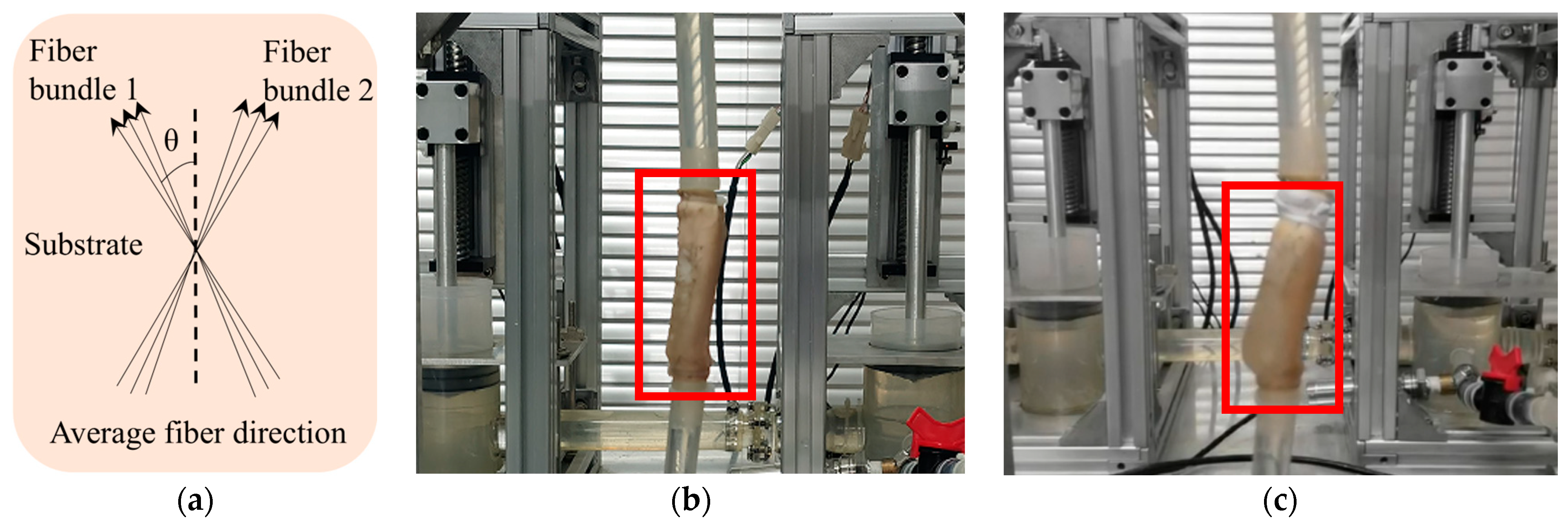
2.1. The Holzapfel–Gasser–Ogden (HGO) Constitutive Model
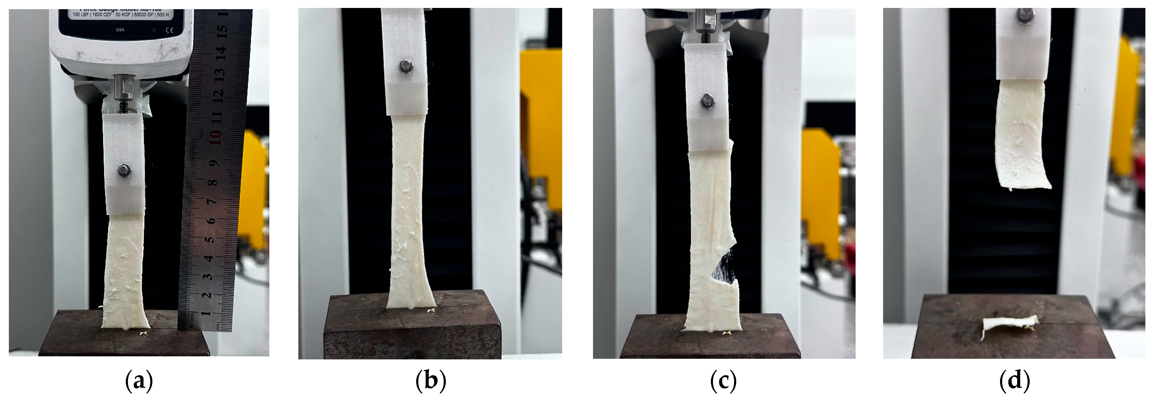
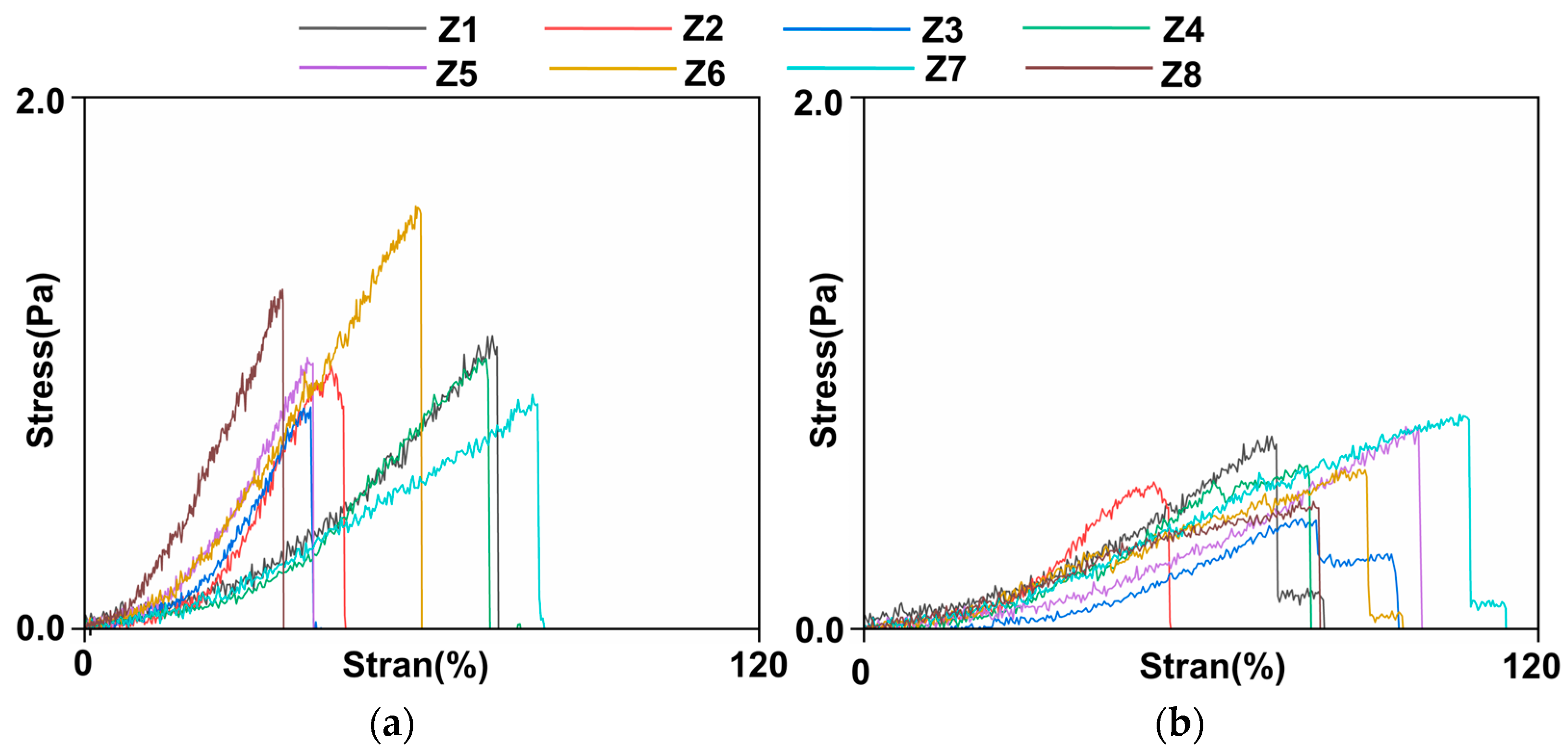
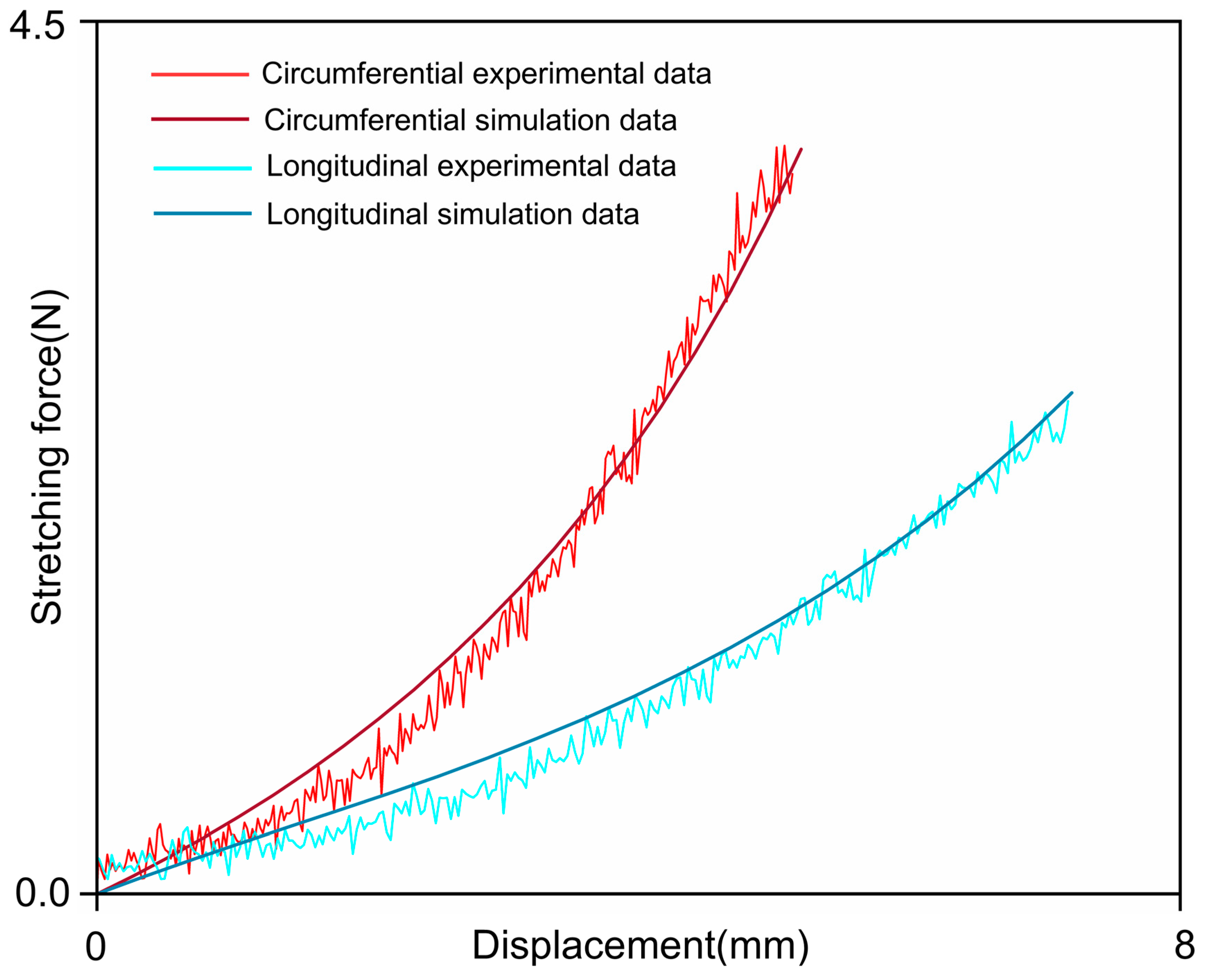
2.2. Establishment of the Constitutive Model
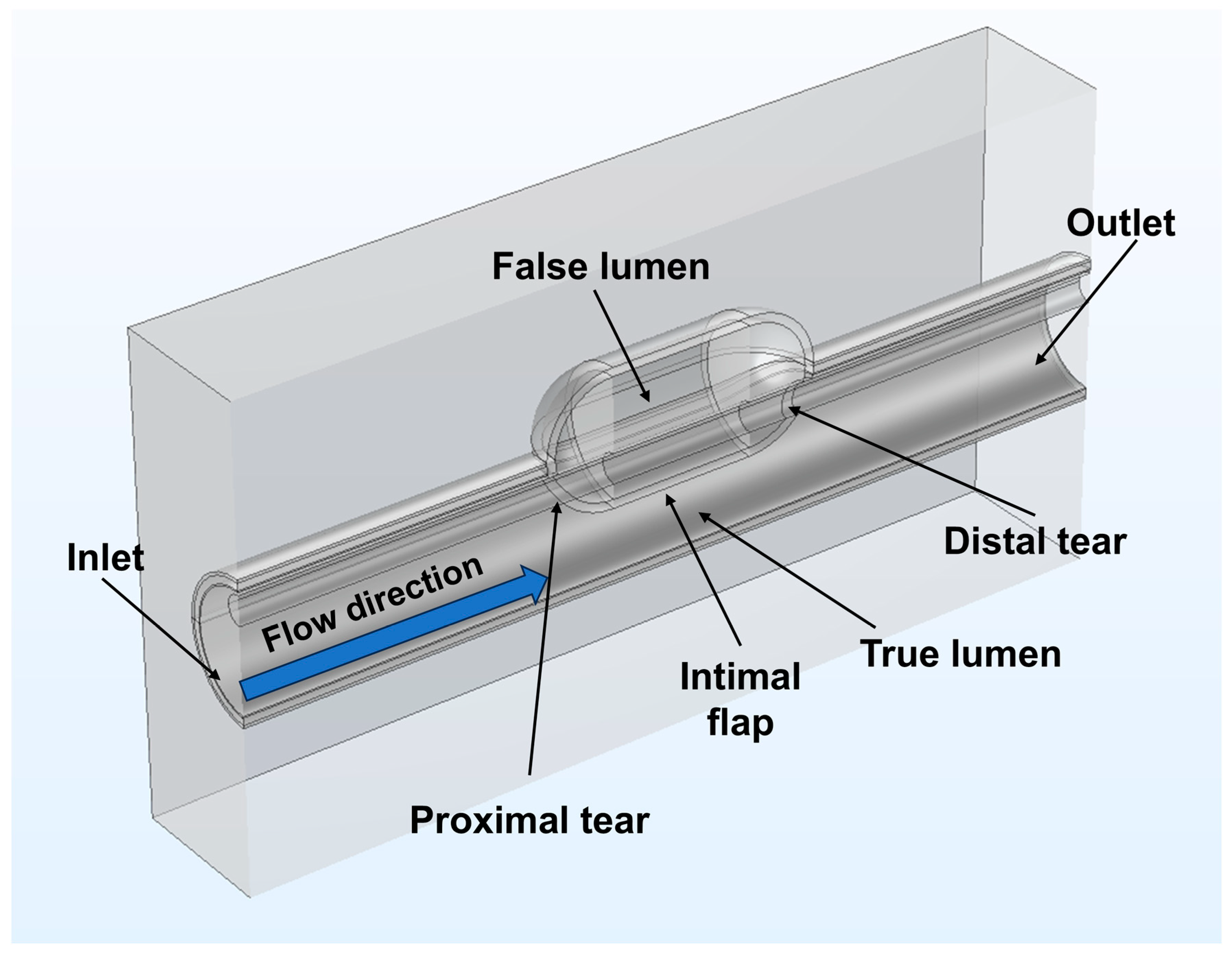
2.3. Establishment of the Geometric Model
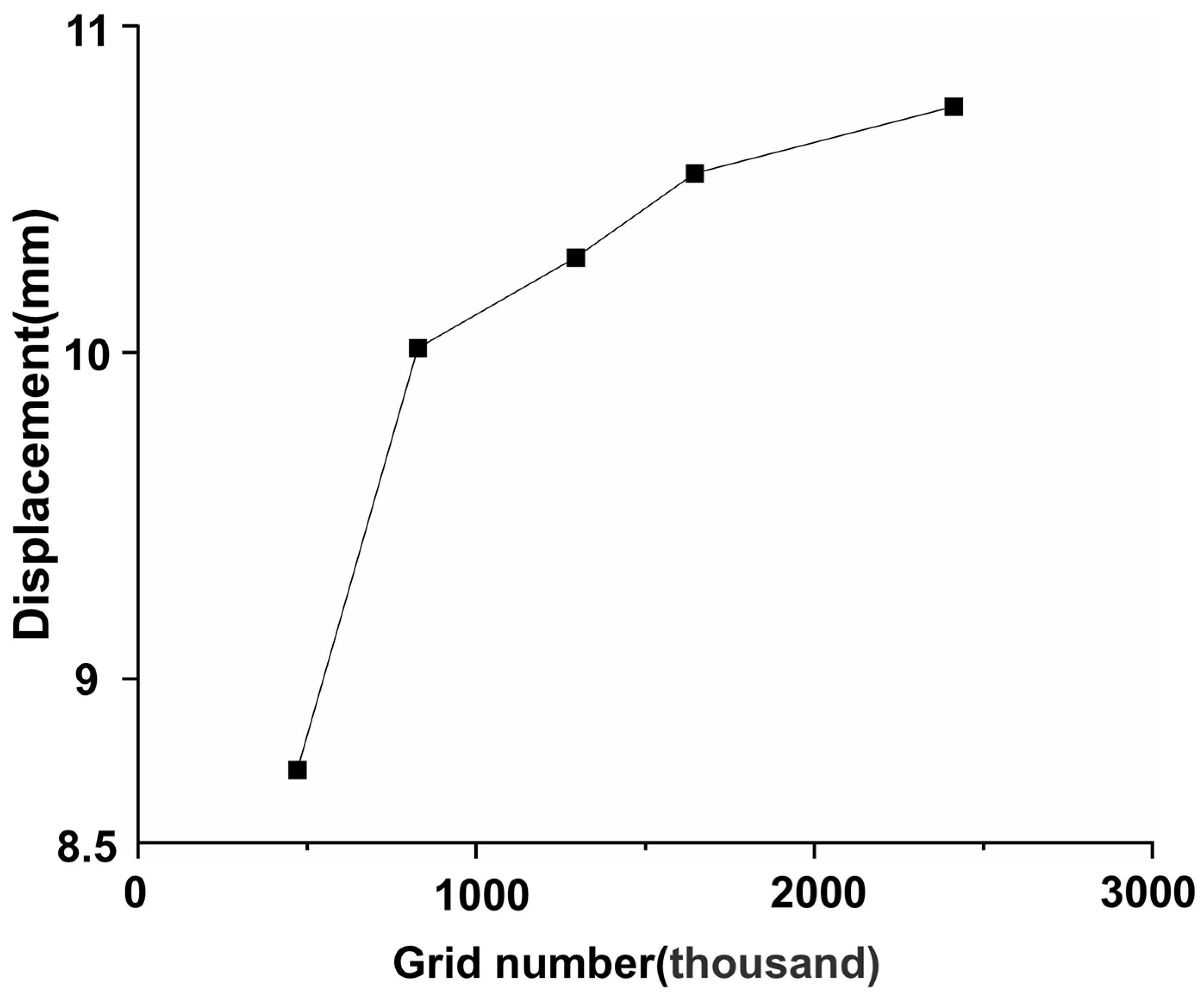
2.4. Mesh Generation and Mesh Independence Test
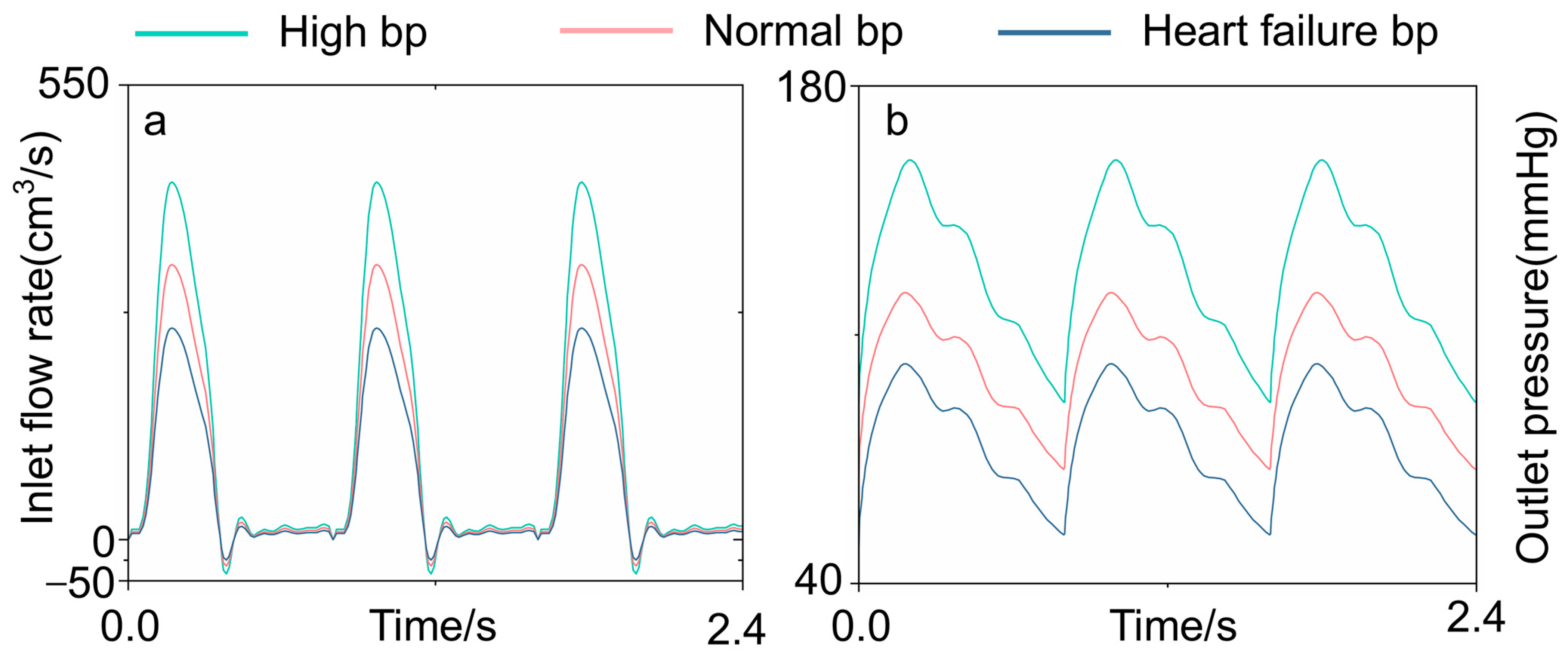
2.5. Blood Property and Simulation Condition Settings
3. Results
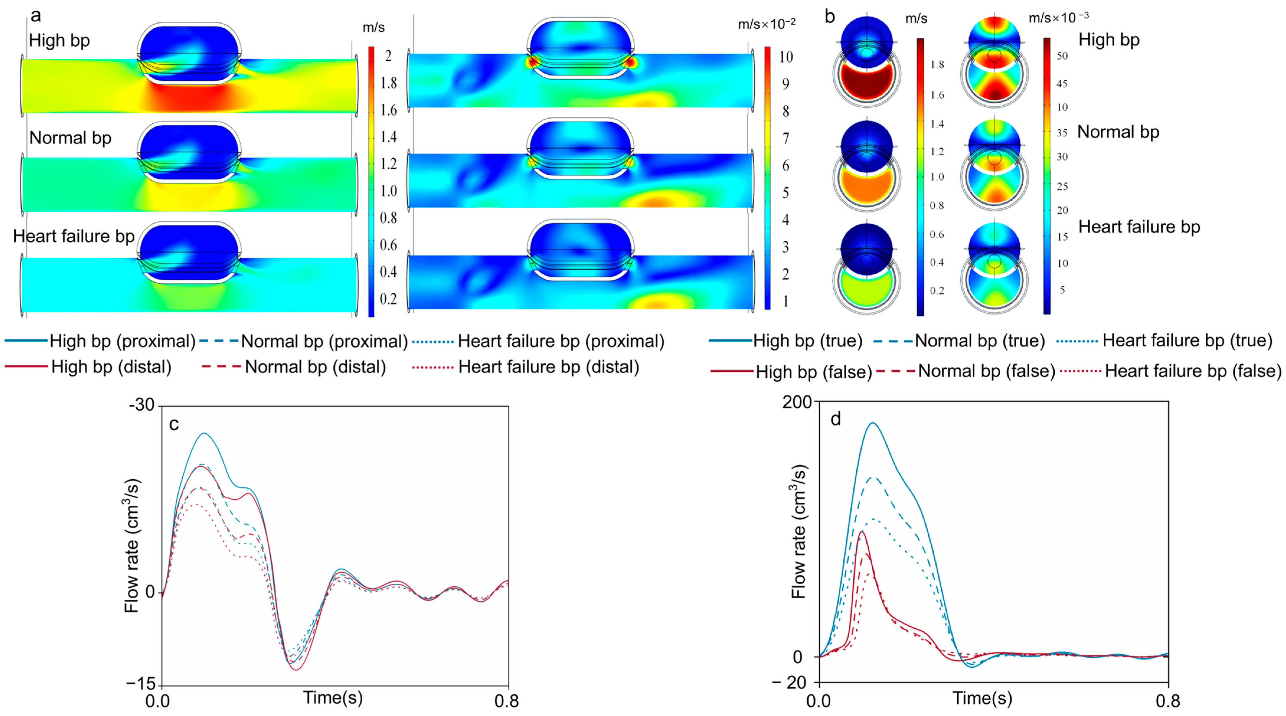
3.1. Velocity Field
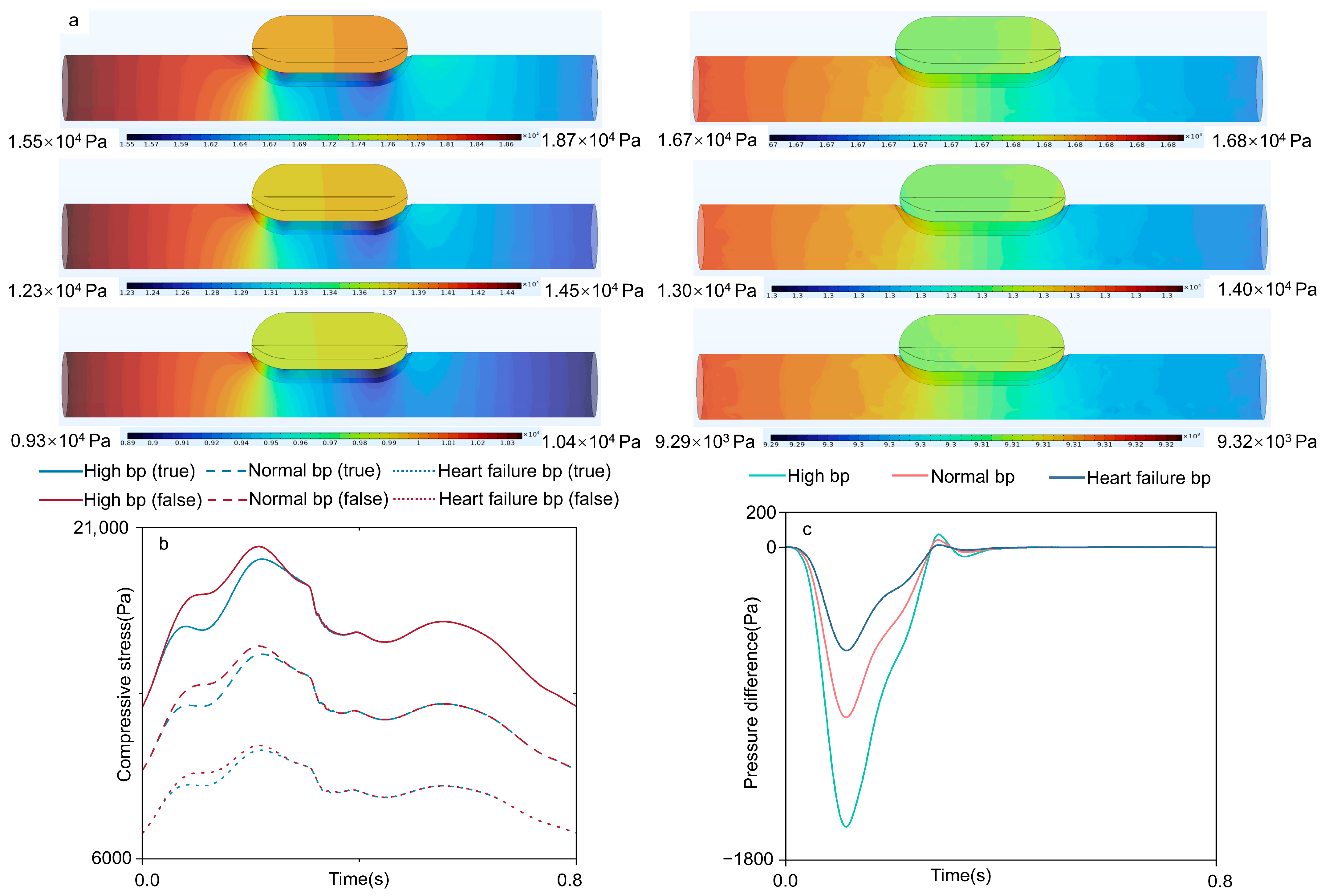
3.2. Compressive Stress
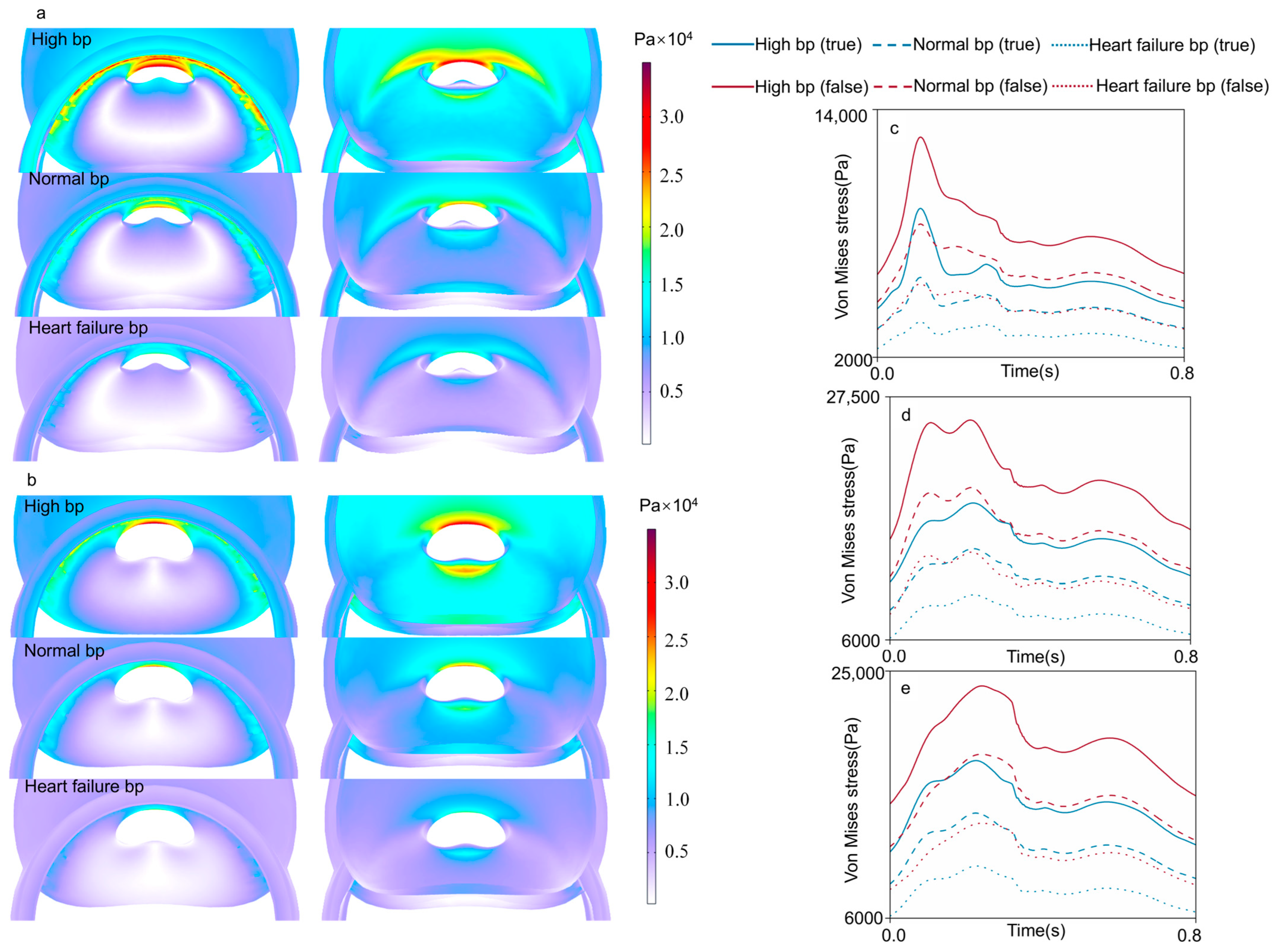
3.3. Von Mises Stress
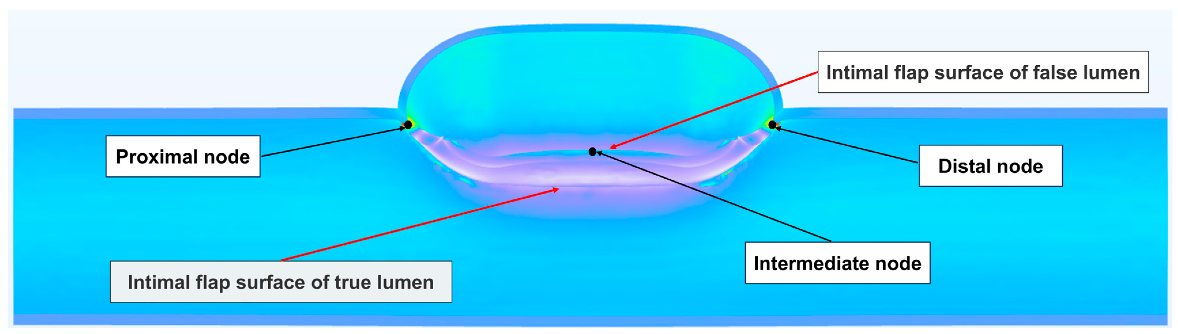
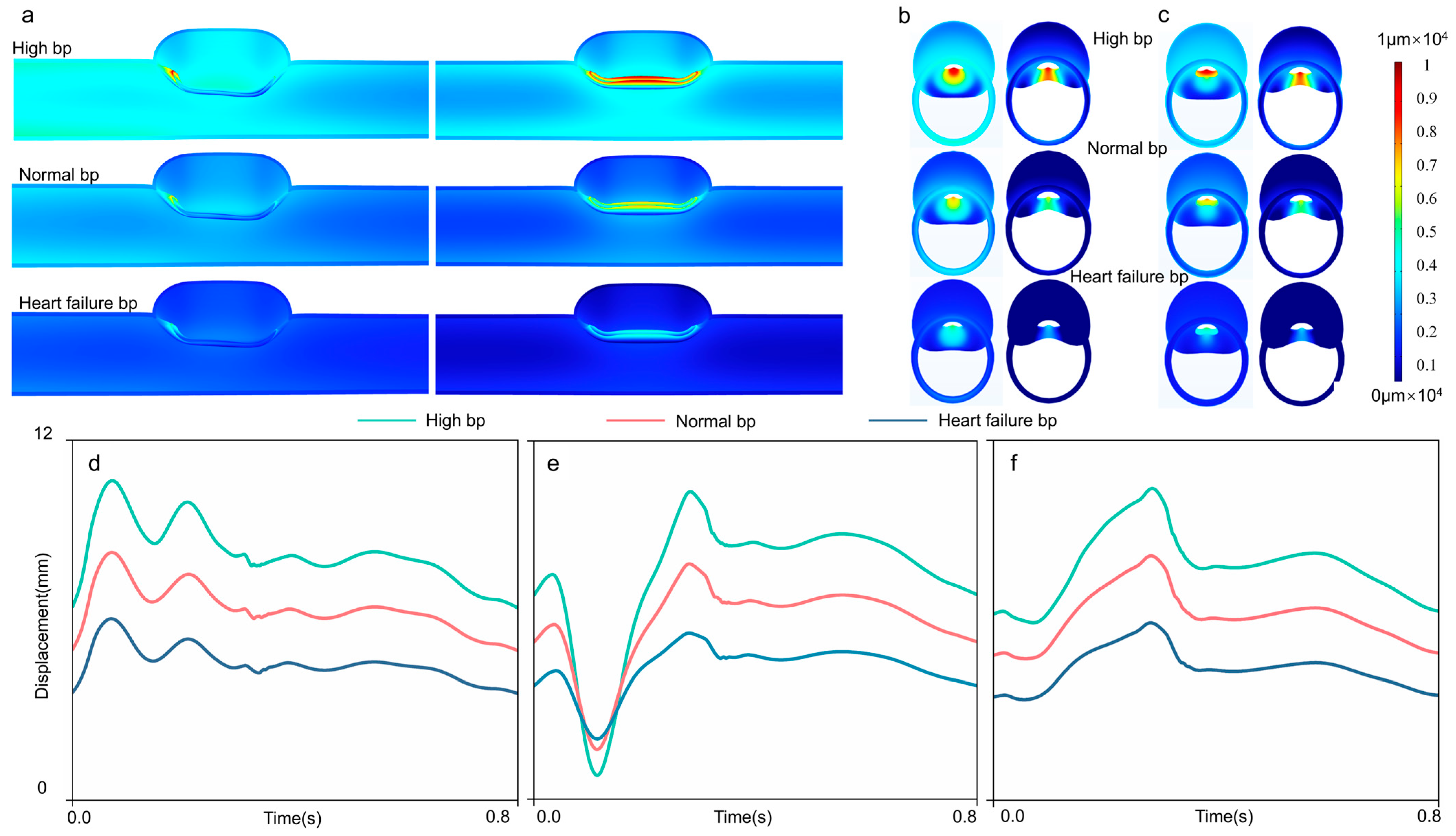
3.4. Intimal Flap Deformation
4. Discussion
4.1. Constitutive Model
4.2. Stress Field Analysis
4.3. Intimal Flap Deformation Analysis
4.4. Mutual Promotion Between Research, AD Pathology, and Clinical Practice
4.5. Limitations and Suggestions for Improvement
5. Conclusions
Author Contributions
Funding
Institutional Review Board Statement
Informed Consent Statement
Data Availability Statement
Conflicts of Interest
Abbreviations
| AD | Aortic dissection |
| TBAD | Stanford type B aortic dissection |
| CFD | Computational fluid dynamics |
| FSI | Fluid–structure interaction |
| bp | Blood flow |
| TL | True lumens |
| FL | False lumens |
References
- Khan, A.; Chaoen, L.; Fan, H.; Shuangxi, H.; Qiaoling, L.; Lei, Z. Study on preoperative treatment of acute Type-a aortic dissection with endotracheal intubation combined with deep analgesia and sedation. Pak. J. Med. Sci. 2024, 40, 46–54. [Google Scholar] [CrossRef] [PubMed]
- Han, Y.; Cui, Y.; Liu, J.; Wang, D.; Zou, G.; Qi, X.; Meng, J.; Huang, X.; He, H.; Li, X. Single-cell rna-seq reveals injuries in aortic dissection and identifies pdgf signalling pathway as a potential therapeutic target. J. Cell. Mol. Med. 2024, 28, e70293. [Google Scholar] [CrossRef] [PubMed]
- Meel, R.; Hasenkam, M.; Goncalves, R.; Blair, K.; Mogaladi, S. Spectrum of ascending aortic aneurysms at a peri-urban tertiary hospital: An echocardiography-based study. Front. Cardiovasc. Med. 2023, 10, 1209969. [Google Scholar] [CrossRef] [PubMed]
- Acosta, S.; Gottsäter, A. Stable population-based incidence of acute type a and b aortic dissection. Scand. Cardiovasc. J. 2019, 53, 274–279. [Google Scholar] [CrossRef]
- Abdelnour, L.H.; Abdalla, M.E.; Elhassan, S.; Kheirelseid, E.A.H. Diabetes, hypertension, smoking, and hyperlipidemia as risk factors for spontaneous cervical artery dissection: Meta-analysis of case-control studies. Curr. J. Neurol. 2022, 21, 183–193. [Google Scholar] [CrossRef] [PubMed]
- Wang, Q.; Yesitayi, G.; Liu, B.; Siti, D.; Ainiwan, M.; Aizitiaili, A.; Ma, X. Targeting metabolism in aortic aneurysm and dissection: From basic research to clinical applications. Int. J. Biol. Sci. 2023, 19, 3869–3891. [Google Scholar] [CrossRef]
- Isselbacher, E.M.; Preventza, O.; Black, J.H., 3rd; Augoustides, J.G.; Beck, A.W.; Bolen, M.A.; Braverman, A.C.; Bray, B.E.; Brown-Zimmerman, M.M.; Chen, E.P.; et al. 2022 acc/aha guideline for the diagnosis and management of aortic disease: A report of the american heart association/american college of cardiology joint committee on clinical practice guidelines. Circulation 2022, 146, e334–e482. [Google Scholar] [CrossRef]
- Humphrey, J.D.; Schwartz, M.A. Vascular mechanobiology: Homeostasis, adaptation, and disease. Annu. Rev. Biomed. Eng. 2021, 23, 1–27. [Google Scholar] [CrossRef]
- Ahuja, A.; Noblet, J.N.; Trudnowski, T.; Patel, B.; Krieger, J.F.; Chambers, S.; Kassab, G.S. Biomechanical material characterization of stanford type-b dissected porcine aortas. Front. Physiol. 2018, 9, 1317. [Google Scholar] [CrossRef]
- Bhat, S.K.; Yamada, H. Mechanical characterization of dissected and dilated human ascending aorta using Fung-type hyperelastic models with pre-identified initial tangent moduli for low-stress distensibility. J. Mech. Behav. Biomed. Mater. 2022, 125, 104959. [Google Scholar] [CrossRef]
- Ab Naim, W.N.W.; Ganesan, P.B.; Sun, Z.; Chee, K.H.; Hashim, S.A.; Lim, E. A Perspective Review on Numerical Simulations of Hemodynamics in Aortic Dissection. Sci. World J. 2014, 2014, 652520. [Google Scholar] [CrossRef]
- Ben Ahmed, S.; Dillon-Murphy, D.; Figueroa, C.A. Computational Study of Anatomical Risk Factors in Idealized Models of Type B Aortic Dissection. J. Vasc. Surg. 2015, 62, 820–821. [Google Scholar] [CrossRef]
- Pan, Y.-Y.; Guan, Z.-Y.; Li, C.-W.; Guan, H.-X. Progression from Initial Lesions to Type B Aortic Dissection: A Patient-Specific Study of Computational Fluid Dynamics Models with Follow-up Data. Curr. Med Sci. 2025, 45, 373–381. [Google Scholar] [CrossRef] [PubMed]
- Wang, J.; Chen, B.; Gao, F. Exploring hemodynamic mechanisms and re-intervention strategies for partial false lumen thrombosis in Stanford type B aortic dissection after thoracic aortic endovascular repair. Int. J. Cardiol. 2024, 417, 132494. [Google Scholar] [CrossRef] [PubMed]
- Tang, A.; Fan, Y.; Cheng, S.; Chow, K. Biomechanical Factors Influencing Type B Thoracic Aortic Dissection: Computational Fluid Dynamics Study. Eng. Appl. Comput. Fluid Mech. 2012, 6, 622–632. [Google Scholar] [CrossRef]
- Wang, W.Q.; Yan, Y.; Zhang, C.L. Numerical simulation of blood pulsatile flow in a debakey III type of tvd. J. Beijing Univ. Technol. 2012, 38, 949–954. [Google Scholar]
- Birjiniuk, J.; Veeraswamy, R.K.; Oshinski, J.N.; Ku, D.N. Intermediate fenestrations reduce flow reversal in a silicone model of Stanford Type B aortic dissection. J. Biomech. 2019, 93, 101–110. [Google Scholar] [CrossRef]
- Keramati, H.; Birgersson, E.; Ho, J.P.; Kim, S.; Chua, K.J.; Leo, H.L. The effect of the entry and re-entry size in the aortic dissection: A two-way fluid–structure interaction simulation. Biomech. Model. Mechanobiol. 2020, 19, 2643–2656. [Google Scholar] [CrossRef]
- Chong, M.Y.; Gu, B.; Chan, B.T.; Ong, Z.C.; Xu, X.Y.; Lim, E. Effect of intimal flap motion on flow in acute type B aortic dissection by using fluid-structure interaction. Int. J. Numer. Methods Biomed. Eng. 2020, 36, e3399. [Google Scholar] [CrossRef]
- Karabelas, E.; Gsell, M.A.; Haase, G.; Plank, G.; Augustin, C.M. An accurate, robust, and efficient finite element framework with applications to anisotropic, nearly and fully incompressible elasticity. Comput. Methods Appl. Mech. Eng. 2022, 394, 114887. [Google Scholar] [CrossRef]
- Fischer, J.; Turčanová, M.; Man, V.; Hermanová, M.; Bednařík, Z.; Burša, J. Importance of experimental evaluation of structural parameters for constitutive modelling of aorta. J. Mech. Behav. Biomed. Mater. 2023, 138, 105615. [Google Scholar] [CrossRef] [PubMed]
- Leng, X.; Chen, X.; Deng, X.; Sutton, M.A.; Lessner, S.M. Modeling of Experimental Atherosclerotic Plaque Delamination. Ann. Biomed. Eng. 2015, 43, 2838–2851. [Google Scholar] [CrossRef] [PubMed]
- de Beaufort, H.W.; Ferrara, A.; Conti, M.; Moll, F.L.; van Herwaarden, J.A.; Figueroa, C.A.; Bismuth, J.; Auricchio, F.; Trimarchi, S. Comparative Analysis of Porcine and Human Thoracic Aortic Stiffness. Eur. J. Vasc. Endovasc. Surg. 2018, 55, 560–566. [Google Scholar] [CrossRef] [PubMed]
- Wang, X.; Carpenter, H.J.; Ghayesh, M.H.; Kotousov, A.; Zander, A.C.; Amabili, M.; Psaltis, P.J. A review on the biomechanical behaviour of the aorta. J. Mech. Behav. Biomed. Mater. 2023, 144, 105922. [Google Scholar] [CrossRef]
- Shen, P.; Wang, Y.; Chen, Y.; Fu, P.; Zhou, L.; Liu, L. Hydrodynamic Bearing Structural Design of Blood Pump Based on Axial Passive Suspension Stability Analysis of Magnetic–Hydrodynamic Hybrid Suspension System. Machines 2021, 9, 255. [Google Scholar] [CrossRef]
- Cheng, Z.; Tan, F.P.P.; Riga, C.V.; Bicknell, C.D.; Hamady, M.S.; Gibbs, R.G.J.; Wood, N.B.; Xu, X.Y. Analysis of Flow Patterns in a Patient-Specific Aortic Dissection Model. J. Biomech. Eng. 2010, 132, 051007. [Google Scholar] [CrossRef]
- Raghavan, M.; Vorp, D.A. Toward a biomechanical tool to evaluate rupture potential of abdominal aortic aneurysm: Identification of a finite strain constitutive model and evaluation of its applicability. J. Biomech. 2000, 33, 475–482. [Google Scholar] [CrossRef]
- Pirola, S.; Guo, B.; Menichini, C.; Saitta, S.; Fu, W.; Dong, Z.; Xu, X.Y. 4-D Flow MRI-Based Computational Analysis of Blood Flow in Patient-Specific Aortic Dissection. IEEE Trans. Biomed. Eng. 2019, 66, 3411–3419. [Google Scholar] [CrossRef]
- Wang, C.; He, X.; Zhang, Z.; Lai, C.; Li, X.; Zhou, Z.; Ruan, K. Three-Dimensional Finite Element Analysis and Biomechanical Analysis of Midfoot von Mises Stress Levels in Flatfoot, Clubfoot, and Lisfranc Joint Injury. Med. Sci. Monit. 2021, 27, e931969. [Google Scholar] [CrossRef]
- Gomez, A.; Wang, Z.; Xuan, Y.; Wisneski, A.D.; Hope, M.D.; Saloner, D.A.; Guccione, J.M.; Ge, L.; Tseng, E.E. Wall Stress Distribution in Bicuspid Aortic Valve–Associated Ascending Thoracic Aortic Aneurysms. Ann. Thorac. Surg. 2020, 110, 807–814. [Google Scholar] [CrossRef]
- Fillinger, M.F.; Marra, S.P.; Raghavan, M.; Kennedy, F.E. Prediction of rupture risk in abdominal aortic aneurysm during observation: Wall stress versus diameter. J. Vasc. Surg. 2003, 37, 724–732. [Google Scholar] [CrossRef] [PubMed]
- Erbel, R.; Eggebrecht, H. Aortic dimensions and the risk of dissection. Heart 2006, 92, 137–142. [Google Scholar] [CrossRef] [PubMed]
- Vuong, T.N.A.M.; Bartolf-Kopp, M.; Andelovic, K.; Jungst, T.; Farbehi, N.; Wise, S.G.; Hayward, C.; Stevens, M.C.; Rnjak-Kovacina, J. Integrating Computational and Biological Hemodynamic Approaches to Improve Modeling of Atherosclerotic Arteries. Adv. Sci. 2024, 11, e2307627. [Google Scholar] [CrossRef]
- Rajagopal, K.; Bridges, C. Towards an understanding of the mechanics underlying aortic dissection. Biomech. Model. Mechanobiol. 2007, 6, 345–359. [Google Scholar] [CrossRef]
- Giannakoulas, G.; Soulis, J.; Farmakis, T.; Papadopoulou, S.; Parcharidis, G.; Louridas, G. A computational model to predict aortic wall stresses in patients with systolic arterial hypertension. Med. Hypotheses 2005, 65, 1191–1195. [Google Scholar] [CrossRef]
- Khanafer, K.; Berguer, R. Fluid–structure interaction analysis of turbulent pulsatile flow within a layered aortic wall as related to aortic dissection. J. Biomech. 2009, 42, 2642–2648. [Google Scholar] [CrossRef]
- Yang, S.; Li, X.; Chao, B.; Wu, L.; Cheng, Z.; Duan, Y.; Wu, D.; Zhan, Y.; Chen, J.; Liu, B.; et al. Abdominal Aortic Intimal Flap Motion Characterization in Acute Aortic Dissection: Assessed with Retrospective ECG-Gated Thoracoabdominal Aorta Dual-Source CT Angiography. PLoS ONE 2014, 9, e87664. [Google Scholar] [CrossRef] [PubMed]
- Bekkaoui, S.; Ben El Mamoun, I.; Berrichi, H.; Oulali, N. Acute total aortic dissection revealed by incoercible vomiting with multiple organ failure a case report. Ann. Med. Surg. 2022, 76, 103518. [Google Scholar] [CrossRef]
- Robicsek, F.; Thubrikar, M.J. Hemodynamic considerations regarding the mechanism and prevention of aortic dissection. Ann. Thorac. Surg. 1994, 58, 1247–1253. [Google Scholar] [CrossRef]
- Peng, X.; Li, Z.; Cai, L.; Li, H.; Zhong, F.; Luo, L. A bioinformatics analysis of the susceptibility genes in Stanford type A aortic dissection. J. Thorac. Dis. 2023, 15, 1694–1703. [Google Scholar] [CrossRef]


| Specimen | C10/MPa | k1/MPa | k2 | θ/° | κ |
|---|---|---|---|---|---|
| Z1 | 0.0935 | 0.3356 | 0.3964 | 31 | 0.1106 |
| Z2 | 0.0311 | 0.5641 | 1.4087 | 40 | 0.0166 |
| Z3 | 0.0858 | 0.5972 | 1.8936 | 23 | 0.2316 |
| Z4 | 0.0750 | 0.5225 | 3.5600 | 46 | 0.3015 |
| Z5 | 0.0847 | 0.5415 | 1.2654 | 13 | 0.2622 |
| Z6 | 0.1477 | 0.7109 | 0.1236 | 25 | 0.2219 |
| Z7 | 0.1495 | 0.1925 | 0.7318 | 60 | 0.3277 |
| Z8 | 0.1182 | 0.5442 | 2.0111 | 25 | 0.1196 |
| Mean value | 0.0982 | 0.5011 | 1.4238 | 32.9 | 0.1990 |
| Standard deviation | 0.0369 | 0.1516 | 1.0234 | 14.1 | 0.1000 |
| Area | C10/MPa | k1/MPa | k2 | θ/° | κ |
|---|---|---|---|---|---|
| Adventitia | 0.0130 | 0.1741 | 0.4847 | 36.6 | 0.2740 |
| Media | 0.1710 | 0.5856 | 3.5447 | 22.6 | 0.2170 |
| Intima | 0.1828 | 0.8984 | 2.5716 | 34.8 | 0.2239 |
| FL wall | 0.1269 | 1.0934 | 5.6109 | 25.1 | 0.2354 |
| Intimal flap | 0.0982 | 0.5011 | 1.4238 | 32.9 | 0.1990 |
| Relaxation Time (s) | Power-Law Index | Yasuda Index | Zero-Shear Viscosity (mPas) | Infinite-Shear Viscosity (mPas) |
|---|---|---|---|---|
| 0.1 | 0.392 | 0.664 | 22 | 2.2 |
| Blood Pressure | Lumen | Mean ± Standard Deviation/Pa | Min/Pa | Max/Pa |
|---|---|---|---|---|
| High | True | 5747.6 ± 1020.5 | 4329.2 | 9207.0 |
| False | 8138.4 ± 1545.8 | 5983.3 | 12,662.0 | |
| Normal | True | 4343.5 ± 521.9 | 3366.9 | 5862.5 |
| False | 6181.8 ± 909.9 | 4653.3 | 8451.4 | |
| Heart failure | True | 3067.5 ± 307.5 | 2404.2 | 3709.6 |
| False | 4368.7 ± 566.9 | 3322.9 | 5551.9 |
| Blood Pressure | Observation Node | Mean ± Standard Deviation/mm | Max/mm | Min/mm |
|---|---|---|---|---|
| High | proximal node | 8.2033 ± 1.0136 | 6.2564 | 10.6450 |
| distal node | 7.7732 ± 1.1528 | 5.9016 | 10.3850 | |
| intermediate node | 7.4394 ± 2.1500 | 0.8004 | 10.2920 | |
| Normal | proximal node | 6.3538 ± 0.7567 | 4.8648 | 8.2431 |
| distal node | 6.0881 ± 0.8894 | 4.7038 | 8.1334 | |
| intermediate node | 5.8543 ± 1.3679 | 1.6623 | 7.8678 | |
| Heart failure | proximal node | 4.5327 ± 0.5581 | 3.4733 | 6.0340 |
| distal node | 4.3692 ± 0.6529 | 3.3475 | 5.8987 | |
| intermediate node | 4.3681 ± 0.7836 | 2.0199 | 5.5504 |
Disclaimer/Publisher’s Note: The statements, opinions and data contained in all publications are solely those of the individual author(s) and contributor(s) and not of MDPI and/or the editor(s). MDPI and/or the editor(s) disclaim responsibility for any injury to people or property resulting from any ideas, methods, instructions or products referred to in the content. |
© 2025 by the authors. Licensee MDPI, Basel, Switzerland. This article is an open access article distributed under the terms and conditions of the Creative Commons Attribution (CC BY) license (https://creativecommons.org/licenses/by/4.0/).
Share and Cite
Wang, Y.; Xin, L.; Zhou, L.; Wu, X.; Zhang, J.; Wang, Z. Biodynamic Characteristics and Blood Pressure Effects of Stanford Type B Aortic Dissection Based on an Accurate Constitutive Model. Appl. Sci. 2025, 15, 5853. https://doi.org/10.3390/app15115853
Wang Y, Xin L, Zhou L, Wu X, Zhang J, Wang Z. Biodynamic Characteristics and Blood Pressure Effects of Stanford Type B Aortic Dissection Based on an Accurate Constitutive Model. Applied Sciences. 2025; 15(11):5853. https://doi.org/10.3390/app15115853
Chicago/Turabian StyleWang, Yiwen, Libo Xin, Lijie Zhou, Xuefeng Wu, Jinong Zhang, and Zhaoqi Wang. 2025. "Biodynamic Characteristics and Blood Pressure Effects of Stanford Type B Aortic Dissection Based on an Accurate Constitutive Model" Applied Sciences 15, no. 11: 5853. https://doi.org/10.3390/app15115853
APA StyleWang, Y., Xin, L., Zhou, L., Wu, X., Zhang, J., & Wang, Z. (2025). Biodynamic Characteristics and Blood Pressure Effects of Stanford Type B Aortic Dissection Based on an Accurate Constitutive Model. Applied Sciences, 15(11), 5853. https://doi.org/10.3390/app15115853