The Effect of Turbulent Intensity on Friction Coefficient in Boundary-Layer Transitional Flat Plate Flow


Abstract
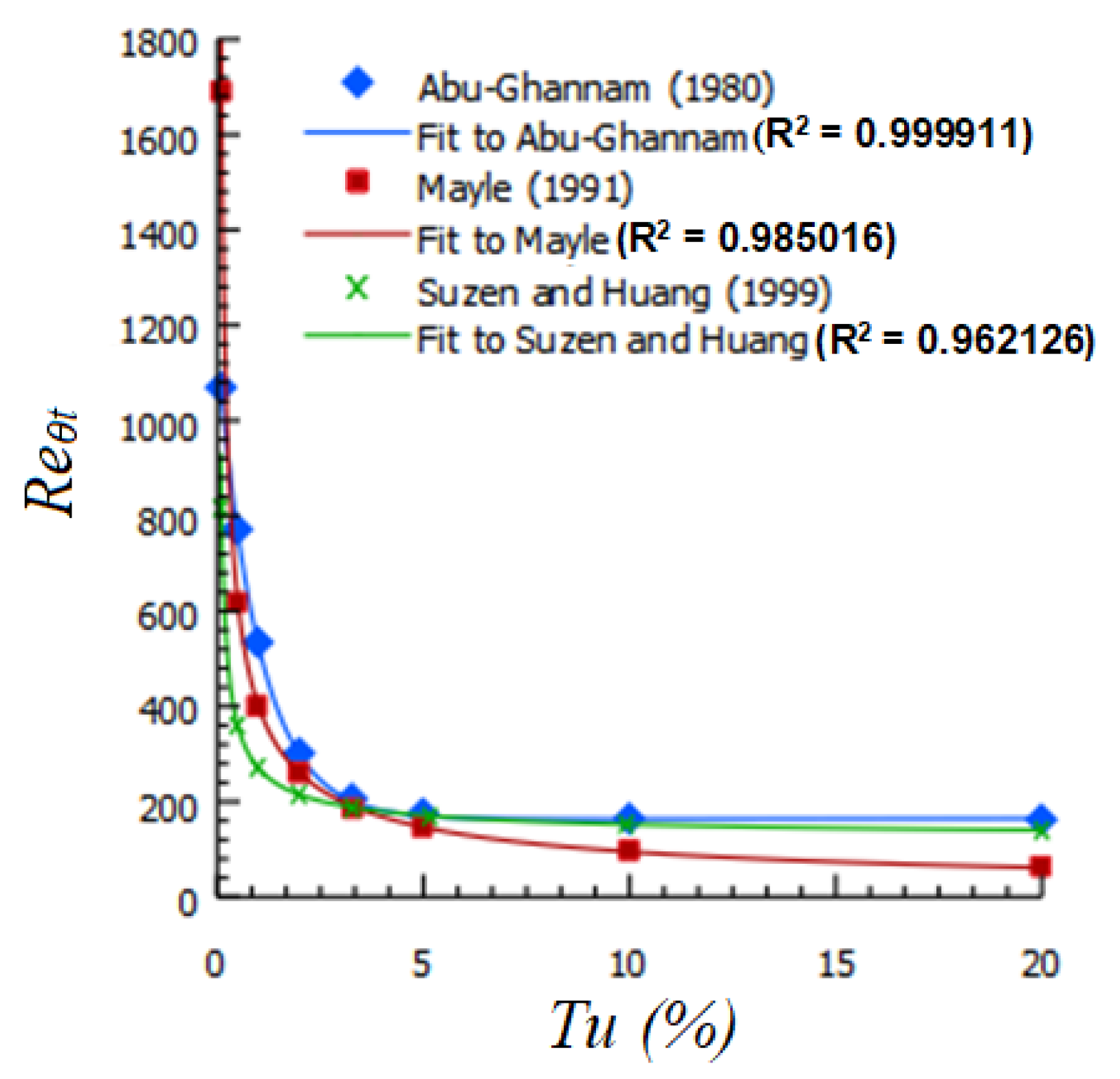
1. Introduction
2. Materials and Methods
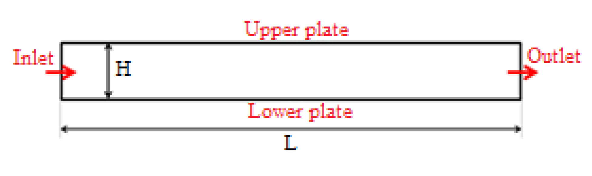
2.1. Geometrical Model and Boundary Conditions
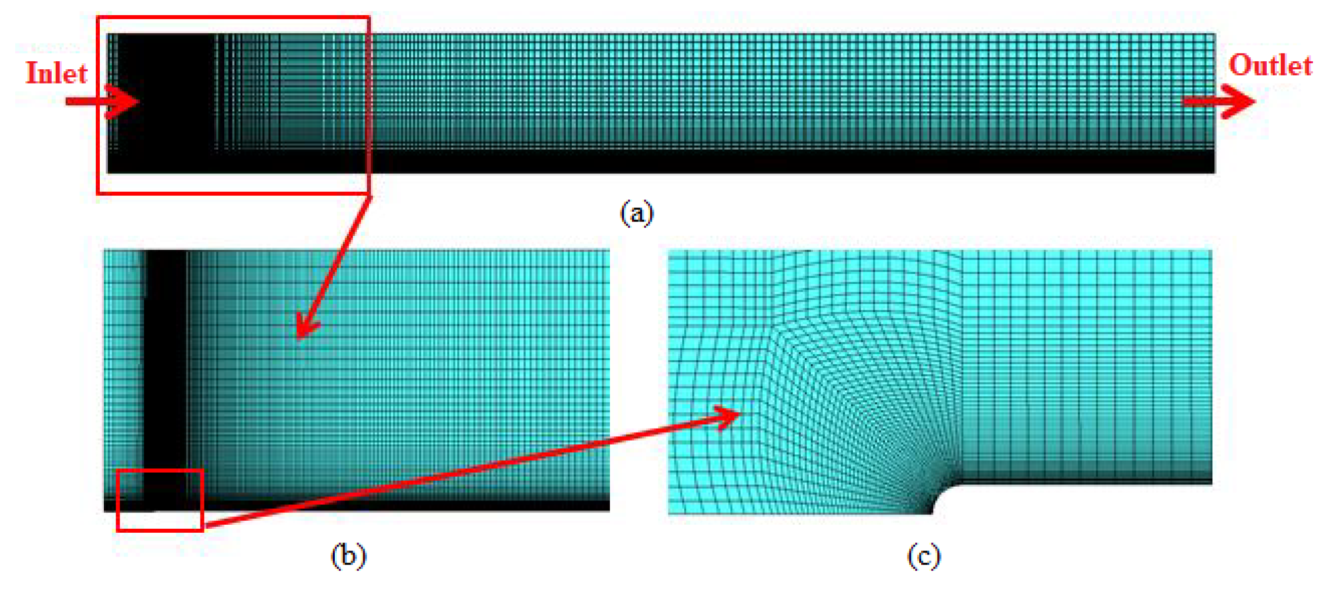
2.2. Mesh Independence Study
2.3. Thermophysical Properties
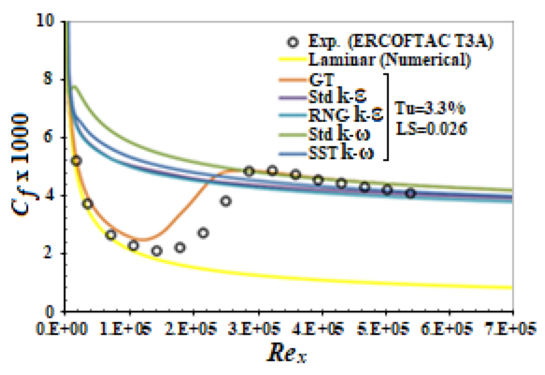
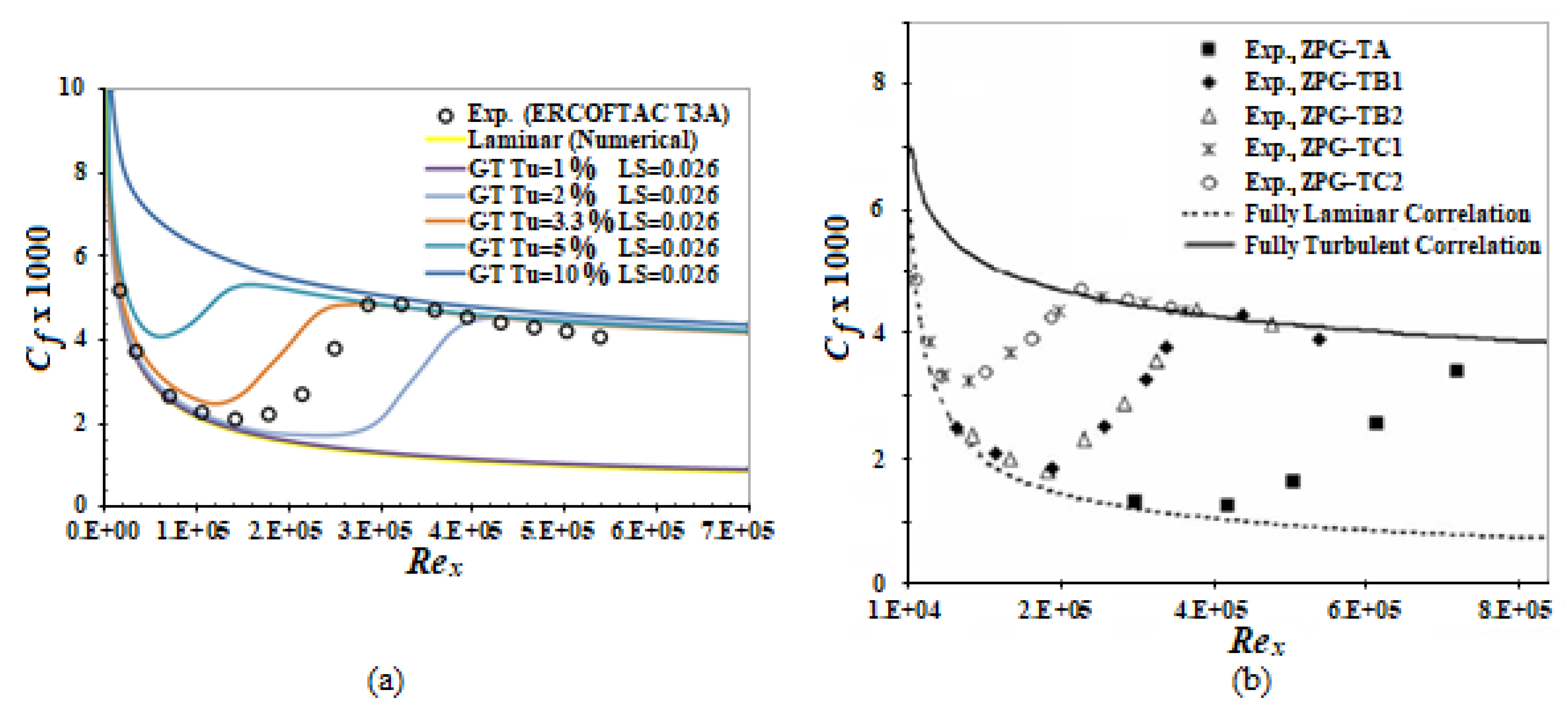
3. Results and Discussion
4. Conclusions
Author Contributions
Funding
Institutional Review Board Statement
Informed Consent Statement
Data Availability Statement
Acknowledgments
Conflicts of Interest
Nomenclature
| ai, bi, ci | Empirically derived constants in Equation (4) |
| Cf | Friction coefficient |
| DNS | Direct numerical simulation |
| GT | Gamma–Theta turbulence model |
| LES | Large-eddy simulation |
| LS | Turbulent-length scale |
| Reϴt | Transition to turbulence Reynolds number (Transitional Reynolds number) |
| Rex | Local Reynolds number |
| Tu | Turbulence intensity |
| ZPG | Zero-pressure gradient |
References
- Emmons, H.W. The laminar-turbulent transition in a boundary layer–part1. J. Aeronaut. Sci. 1951, 18, 490–498. [Google Scholar] [CrossRef]
- Kestin, J.; Maeder, P.F.; Wang, H.E. Influence of turbulence on the transfer of heat from plates with and without a pressure gradient. Int. J. Heat Mass Transf. 1961, 3, 133–154. [Google Scholar] [CrossRef]
- Büyüktür, A.R.; Kestin, J.; Maeder, P.F. Influence of combined pressure gradient and turbulence on the transfer of heat from a plate. Int. J. Heat Mass Transf. 1964, 7, 1175–1184. [Google Scholar] [CrossRef]
- Simonich, J.C.; Bradshaw, P. Effect of free-stream turbulence on heat transfer through a turbulent boundary layer. J. Heat Transf.-Trans. ASME 1978, 100, 671–677. [Google Scholar] [CrossRef]
- Maciejewski, P.K.; Moffat, R.J. Heat transfer with very high free stream turbulence: Part 1-Experimental data. J. Heat Transf.-Trans. ASME 1992, 114, 827–833. [Google Scholar] [CrossRef]
- Maciejewski, P.K.; Moffat, R.J. Heat transfer with very high free stream turbulence: Part 2-Analysis of results. J. Heat Transf.-Trans. ASME 1992, 114, 834–839. [Google Scholar] [CrossRef]
- Blair, M.F. Influence of free-stream turbulence on turbulent boundary layer heat transfer and mean profile development, Part 1-Experimental data. J. Heat Transf.-Trans. ASME 1983, 105, 33–40. [Google Scholar] [CrossRef]
- Blair, M.F. Influence of free-stream turbulence on turbulent boundary layer heat transfer and mean profile development, Part II-Analysis of results. J. Heat Transf.-Trans. ASME 1983, 105, 41–47. [Google Scholar] [CrossRef]
- Wisler, D.C. The Technical and Economic Relevance of Understanding Boundary Layer Transition in Gas Turbine Engines. In Proceedings of the Minnowbrook II 1997 Workshop on Boundary Layer Transition in Turbomachine, New York, NY, USA, 7–10 September 1997; NASA: Linthicum Heights, MD, USA, 1997; p. CP-1998-206958. [Google Scholar]
- Suzen, Y.; Huang, P.G. Modelling of flow transition: Fundamentals. In Special Course on Skin Friction Drag Reduction (Reduction de Trainee de Frottement); NATO: Brussels, Belgium, 1999; p. AGARD-R-786. [Google Scholar]
- Saric, W.F. Laminar-turbulent transition: Fundamentals. In Special Course on Skin Friction Drag Reduction (Reduction de Trainee de Frottement); NATO: Brussels, Belgium, 1992; p. AGARD-R-786. [Google Scholar]
- Mayle, R.E. The role of laminar-turbulent transition in gas turbine engines. J. Turbomach.-Trans. ASME 1991, 113, 509–536. [Google Scholar] [CrossRef]
- Schlichting, H. Boundary Layer Theory; McGraw-Hill: New York, NY, USA, 1979. [Google Scholar]
- Menter, E.R.; Langtry, R.B.; Likki, S.R.; Suzen, Y.B.; Huang, P.G.; Völker, S. A Correlation-based transition model using local variables-Part 1: Model formulation. J. Turbomach.-Trans. ASME 2006, 128, 413–422. [Google Scholar] [CrossRef]
- Radmehr, A.; Patankar, S.V. Computation of boundary layer transition using low-Reynolds number Turbulence Models. Numer. Heat Transf. Part B 2001, 39, 525–543. [Google Scholar]
- Radmehr, A.; Patankar, S.V. A new low-Reynolds number Turbulence Model for prediction of transition on gas turbine blades. Numer. Heat Transf. Part B 2001, 39, 545–562. [Google Scholar]
- Lardeau, S.; Leschziner, M.A.; Li, N. Modelling bypass transition with low-Reynolds-number nonlinear eddy-viscosity closure. Flow Turbul. Combust. 2004, 73, 49–76. [Google Scholar] [CrossRef]
- Langtry, R.B. A Correlation Based Transition Model Using Local Variables for Unstuctured Parallelized CFD Codes. Ph.D. Thesis, Universitat Stuttgart, Stuttgart, Germany, 2006. [Google Scholar]
- Luo, J.; Razinsky, E.H. Conjugate heat transfer analysis of a cooled turbine vane using the V2F Turbulence model. J. Turbomach.-Trans. ASME 2007, 129, 773–781. [Google Scholar] [CrossRef]
- Akhter, M.N.; Yamada, K.; Funazaki, K. Numerical simulation of bypass transition by the approach of intermittency transport equation. J. Fluid Sci. Technol. 2009, 4, 524–535. [Google Scholar] [CrossRef]
- Bochon, K.; Wroblewski, W.; Dykas, S. Modelling of influence of turbulent transition on heat transfer conditions. Task Q. 2008, 12, 173–184. [Google Scholar]
- Piotrowski, W.; Elsner, W.; Drobniak, S. Transition prediction on turbine blade profile with intermittency transport equation. J. Turbomach.-Trans. ASME 2008, 132, 011020. [Google Scholar] [CrossRef]
- Suluksna, K.; Juntasaro, E. Assessment of intermittency transport equations for modeling transition in boundary layers subjected to freestream turbulence. Int. J. Heat Fluid Flow 2008, 29, 48–61. [Google Scholar] [CrossRef]
- Abu-Ghannam, B.; Shaw, R. Natural transition of boundary layers-the effects of turbulence, pressure gradient and flow history. J. Mech. Eng. Sci. 1980, 22, 213–228. [Google Scholar] [CrossRef]
- Taghavi-Zenous, R.; Salari, M.; Tabar, M.M.; Omidi, E. Hot-wire anemometry of transitional boundary layers exposed to different freestream turbulence intensities. Proc. Inst. Mech. Eng. Part G J. Aerosp. Eng. 2008, 222, 347–356. [Google Scholar] [CrossRef]
- Bhushan, S.; Walters, D.K. Development of Parallel Pseudo-Spectral Solver Using Influence Matrix Method and Application to Boundary Layer Transition. Eng. Appl. Comput. Fluid Mech. 2014, 8, 158–177. [Google Scholar] [CrossRef]
- Fabrizio, M. Critical Phenomena in laminar-turbulence transitions by a mean field model. Meccanica 2014, 49, 2079–2086. [Google Scholar] [CrossRef]
- Vizinho, R.; Pascoa, J.; Silvestre, M. Turbulent transition modeling through mechanical considerations. Appl. Math. Comput. 2015, 269, 308–325. [Google Scholar] [CrossRef]
- Subaşı, A.; Güneş, H. Effects of wall heating on boundary layer transition over a flat plate. J. Therm. Sci. Technol. 2015, 35, 59–68. [Google Scholar]
- Abdollahzadeh, M.; Esmaeilpour, M.; Vizinho, R.; Younesi, A.; Pascoa, J.C. Assessment of RANS turbulence models for numerical study of laminar-turbulent transition in convection heat transfer. Int. J. Heat Mass Transf. 2017, 115, 1288–1308. [Google Scholar] [CrossRef]
- Medina, H.; Beechook, A.; Fadhila, H.; Aleksandrova, S.; Benjamin, S. A novel laminar kinetic energy model for the prediction of pretransitional velocity fluctuations and boundary layer transit ion. Int. J. Heat Fluid Flow 2018, 69, 150–163. [Google Scholar] [CrossRef]
- Lienhard, J.H. Heat transfer in flat-plate boundary layers: A correlation for laminar, transitional, and turbulrnt flow. J. Heat Transf.-Trans. ASME 2020, 142, 061805. [Google Scholar] [CrossRef]
- Dotto, A.; Barsi, D.; Lengani, D.; Simoni, D.; Satta, F. Effect of free-stream turbulence properties on different transition routes for a zero-pressure gradient boundary layer. Phys. Fluids 2022, 34, 054102. [Google Scholar] [CrossRef]
- Mamidala, S.B.; Weingartner, A.; Fransson, J.H.M. A comparative study of experiments with numerical simulations of free-stream turbulence transition. J. Fluid Mech. 2022, 951, A46. [Google Scholar] [CrossRef]
- Durovic, K.; Hanifi, A.; Schlatter, P.; Sasaki, K.; Henningson, D.S. Direct numerical simulation of transition under free-stream turbulence and the influence of large integral length scales. Phys. Fluids 2024, 36, 74105. [Google Scholar] [CrossRef]
- Langtry, R.B.; Menter, M.R. Transitional Modeling of General CFD Applications in Aeronautics. In Proceedings of the 43rd AIAA Aerospace Sciences Meeting and Exhibit, Reno, Nevada, 10–13 January 2005. [Google Scholar]
- Erşan, H.A. Numerical Investigation of the Effects of the Outer Turbulence in Fluid Flow and Heat Transfer Characteristics. Master’s Thesis, School of Natural and Applied Sciences, Mechanical Engineering Department, Uludag University, Bursa, Türkiye, 2012. [Google Scholar]
- ANSYS. CFX R13 Modelling Guide; ANSYS: Canonsburg, PA, USA, 2010. [Google Scholar]
- Incropera, F.P.; DeWitt, D.P. Fundamentals of Heat and Mass Transfer; Wiley: Hoboken, NJ, USA, 2003. [Google Scholar]
- Hancock, P.E.; Bradshaw, P. The effect of free-stream turbulence on turbulent boundary layers. J. Fluids Eng.-Trans. ASME 1983, 105, 284–289. [Google Scholar] [CrossRef]
- Iyer, G.R.; Yavuzkurt, S. Comparison of low Reynolds number k-ε models in simulation of momentum and heat transport under high free stream turbulence. Int. J. Heat Mass Transf. 1999, 42, 723–737. [Google Scholar] [CrossRef]
- Jonas, P.; Mazur, O.; Uruba, V. On the receptivity of the by-pass transition to the length scale of the outer stream turbulence. Eur. J. Mech. B Fluids 2000, 19, 707–722. [Google Scholar] [CrossRef]
- Darag, S.A.; Horak, V. Effect of free-stream turbulence properties on boundary layer laminar-turbulent transition: A new approach. AIP Conf. Proc. 2012, 1493, 282–289. [Google Scholar] [CrossRef]


| Density | 1.116 kg/m3 |
| Viscosity | 1.725 Pa.s |
| Conductivity | 0.02428 W/mK |
| Specific heat | 1003.8 J/kgK |
| Tu (%) | LS (m) | Inlet Velocity (m/s) | Laminar Region | Transition Region of Turbulence | Turbulent Region |
|---|---|---|---|---|---|
| 1 | 0.026 | 5.3 | 0 < Re < ∞ | - | - |
| 2 | 0.026 | 5.3 | Re < 280,000 | 280,000 < Re < 400,000 | Re > 400,000 |
| 3.3 | 0.026 | 5.3 | Re < 115,000 | 115,000 < Re < 260,000 | Re > 260,000 |
| 5 | 0.026 | 5.3 | Re < 60,000 | 60,000 < Re < 150,000 | Re > 150,000 |
| 10 | 0.026 | 5.3 | - | - | 0 < Re < ∞ |
| Deney Kodu | Tu (%) | LS (m) | Inlet Velocity (m/s) |
|---|---|---|---|
| ZPG-TA | 1.5 | 0.009 | 15.5 |
| ZPG-TB1 | 3.2 | 0.0105 | 12 |
| ZPG-TB2 | 3.3 | 0.011 | 15 |
| ZPG-TC1 | 4.3 | 0.0126 | 8.35 |
| ZPG-TC2 | 4.4 | 0.0129 | 10.5 |
Disclaimer/Publisher’s Note: The statements, opinions and data contained in all publications are solely those of the individual author(s) and contributor(s) and not of MDPI and/or the editor(s). MDPI and/or the editor(s) disclaim responsibility for any injury to people or property resulting from any ideas, methods, instructions or products referred to in the content. |
© 2025 by the authors. Licensee MDPI, Basel, Switzerland. This article is an open access article distributed under the terms and conditions of the Creative Commons Attribution (CC BY) license (https://creativecommons.org/licenses/by/4.0/).
Share and Cite
Saru, M.; Erşan, H.A.; Pulat, E. The Effect of Turbulent Intensity on Friction Coefficient in Boundary-Layer Transitional Flat Plate Flow. Appl. Sci. 2025, 15, 5852. https://doi.org/10.3390/app15115852
Saru M, Erşan HA, Pulat E. The Effect of Turbulent Intensity on Friction Coefficient in Boundary-Layer Transitional Flat Plate Flow. Applied Sciences. 2025; 15(11):5852. https://doi.org/10.3390/app15115852
Chicago/Turabian StyleSaru, Muhsine, Hıfzı Arda Erşan, and Erhan Pulat. 2025. "The Effect of Turbulent Intensity on Friction Coefficient in Boundary-Layer Transitional Flat Plate Flow" Applied Sciences 15, no. 11: 5852. https://doi.org/10.3390/app15115852
APA StyleSaru, M., Erşan, H. A., & Pulat, E. (2025). The Effect of Turbulent Intensity on Friction Coefficient in Boundary-Layer Transitional Flat Plate Flow. Applied Sciences, 15(11), 5852. https://doi.org/10.3390/app15115852