Article

Experimental Study of the Air Demand of a Spillway Tunnel with Multiple Air Vents

State Key Laboratory of Hydraulics and Mountain River Engineering, Chengdu 610065, China
*
Author to whom correspondence should be addressed.
These authors contributed equally to this work.
Appl. Sci. 2025, 15(11), 5831; https://doi.org/10.3390/app15115831
Submission received: 2 March 2025 / Revised: 30 April 2025 / Accepted: 21 May 2025 / Published: 22 May 2025

Abstract

:
Accurate prediction of air demand in free-surface flows through high-head spillway tunnels with multiple vents represents a critical design challenge. Existing empirical formulas for estimating air demand, derived from studies of single vents using experimental and prototype data, are not directly applicable to multi-vent configurations. This study investigates the combined effects of key parameters on ventilation requirements: (1) flow characteristics (velocity range of 6–12 m/s and depth varying between 0.06 and 0.1 m); (2) vent geometry (total vent area from 28 to 140 cm2 and spatial distribution). Through an experimental analysis, an empirical formula is derived to correlate wall roughness with interfacial shear stress, enabling an improved method for estimating air demand in spillway tunnels with multiple air vents. The resulting predictive model achieves ±25% agreement with two prototype case studies and model tests. These experimentally validated relationships provide quantitative guidelines for optimizing ventilation system designs.

1. Introduction

Spillway tunnels are placed inside dam bodies to regulate the level of the reservoir water and flush the sedimentation of the reservoir [1]. Spillway tunnels are normally divided into a pressurized portion controlled by a sluice gate and an outlet tunnel that discharges the flow into the atmosphere [2]. Gao and Xu defined six flow patterns for an outlet tunnel: (i) subcritical free-surface flow with a small Froude number; (ii) supercritical free-surface flow with a large Froude number; (iii) hydraulic jump with a free-surface flow; (iv) hydraulic jump with a pressurized flow, leading to choking; (v) pressurized flow in the full tunnel, occurring for a hydraulic jump close to the sluice gate; and (vi) pressurized flow in the front part and free-surface flow in the rear part, leading to unstable flow on steep slopes [3,4]. High-velocity free-surface flows under turbulent conditions induce substantial air entrainment, generating pronounced negative pressure gradients in confined tunnel environments. Insufficient ventilation to offset this aerodynamic demand leads to critically low-pressure zones, intensifying operational risks such as structural gate oscillations, cavitation erosion, and transient water hammer effects. These issues introduce greater uncertainties and complexities in dam engineering [5,6,7]. In practical hydraulic engineering applications, spillway tunnels with multiple vents are systematically optimized through aerodynamic design modifications to maintain stable free-surface flow. Therefore, it is essential to study the factors influencing the air demand and air pressure fields under free-surface flow and optimize the design of air vents to avoid these problems and excessive project costs.
Kalinske and Robertson conducted the first systematic study on the air demand ( Q a ) in circular conduits. Their work examined the influence of the pipe slope on air entrainment and proposed a semi-empirical relationship linking air discharge to the Froude number at the gate ( Fr o ) [8]. Over the subsequent three decades, researchers including Campbell, Wisner, and Sharma systematically developed empirical air demand equations for distinct flow regimes, utilizing combined datasets from scaled model experiments and field prototype measurements. These formulations explicitly incorporated the Froude number at the vena contracta ( Fr c ) as a governing hydraulic parameter [9,10,11]. We estimate an error of ±15 to 30% by applying the listed formulas, which still leaves a lot of variability unexplained, and the remaining differences in air demand are attributed primarily to the effects of the characteristics of the air vent and the geometry of the tunnel. Speerli and Hohermuth established a comprehensive empirical formula to predict the air demand of a single air vent, summarizing the other governing parameters as the variable loss coefficient ( δ ) and area (a) of the air vent, tunnel length (L), and slope (S) [2,12].
The empirical models mentioned above cannot accurately clarify the effects of hydraulic and structural factors on air demand, so few researchers have established analytical models through the conservation of mass, momentum, and energy. Luo revised the expression for the interfacial drag coefficient (f) on the basis of prototype observations from 11 projects, and introduced an equation for calculating air demand on the basis of the momentum equation, including the influence of hydraulic and structural factors [13,14]. Lian et al. proposed an air–water stratified flow model to calculate the air demand of air vents, and the model was verified with prototype data from the spillway tunnel of the Jinping-I hydraulic project and numerical CFD results [15,16]. The relationships between air discharge and the effects of hydraulic and structural factors can be quantified on the basis of the empirical and analysis equations listed in Table 1.
CFD simulations have been widely adopted by many researchers to investigate the air characteristics of spillway tunnels [7,15]. Yazdi and Zarrati employed the VOF model on both circular and rectangular tunnels. Using the results of the numerical model, they calculated the air demand and validated it with available experimental data [17]. However, such models grossly overestimate the turbulent viscosity of the free surface and mispredict the velocity close to the air–water interface [18,19,20]. Therefore, a proper two-phase model is necessary to accurately determine the drag forces to study the air demand of a spillway tunnel. Zhang employed the Euler–Euler approach to simulate air discharge through tunnels. The results revealed that the Euler–Euler approach is more accurate than the VOF model in determining drag forces and calculating air demand, which was validated by available experimental data [21]. Salazar used a particle finite element method to model the air–water interaction at a bottom outlet at Susqueda Dam, which was validated by the information gathered on site during gate operation tests [22]. While CFD methods require high-fidelity modeling of drag-induced air entrainment and substantial computational effort—particularly for free-surface flows with multiple ventilation ports—the experimental methodology proposed herein enables rapid, precise air demand estimation, offering practical advantages for real-time engineering assessments.
Current methodological frameworks—including empirical models (Table 1), analytical solutions (Table 1), and CFD simulations (discussed in the preceding section)—demonstrate constrained applicability across diverse engineering applications. This limitation primarily stems from their dependence on narrowly scoped experimental data and project-specific prototype parameters. For example, the empirical model has strict application conditions; the existing analysis model focuses on spillway tunnels that have a single air vent immediately downstream of the gate; CFD models can simulate only the air characteristics of spillway tunnels with an applicable theoretical model and a large amount of computational resources (time and computational power). This paper focuses on the governing parameters of air characteristics of a spillway tunnel with multiple air vents, advancing the mechanistic understanding of air–water interactions in such systems. To achieve this objective, a hydraulic model experiment that allowed for the variation of hydraulic factors (such as flow velocity and water depth) within a certain range, as well as adjustments to structural parameters including the cross-sectional area and position of the vent, was used. Through analysis of the experimental data, we developed a predictive air demand equation that quantitatively integrates the coupled effects of these critical hydraulic and geometric parameters.

2. Experimental Setup

2.1. Model and Instrumentation

A physical model of a typical spillway tunnel was built at the State Key Laboratory of Hydraulics and Mountain River Engineering (SKLH). The model comprises a pressurized section, a gate chamber, an open-channel section, and a tailwater channel section (Figure 1). The pressurized section had a circular cross-section with a diameter of 35 cm, tapering into a square cross-section of 0.35 m × 0.15 m. A plain gate without gate slots was installed to regulate the flow depth ( h w ), ranging from 0.04 m to 0.10 m. The open flow section of the spillway tunnel model had a length (L) of 8 m, a width B of 0.35 m, and a height (h) of 0.16 m for the downstream tunnel section, with a slope (S) of 0.03. All the channel walls were glass with a hydraulic roughness of 12 μ m, and the hydraulic roughness ( Δ ) of the invert was adjusted by placing different grades of sandpaper ranging from 12 μ m to 240 μ m. The three air vents (#1, #2, #3) in the open-flow section had a height ( h a ) of 1.47 m, width ( B a ) of 0.07 m, and length ( L a ) ranging from 0.04 m to 0.20 m and were installed at different positions ( X 2 and X 3 ) of the open-flow section. Prior to the experiments, all sensors underwent three-stage calibration: factory calibration with NIST-traceable standards; pre-experiment verification using reference instruments; and post-experiment drift checks, showing <0.5% deviation. All measurements were conducted under identical conditions, with each parameter recorded 20 times and averaged to ensure reliability. Air velocity ( U a , i ) and air discharge ( Q a , i ) were measured using a GM8903 thermal anemometer (range: 0.1–30 m/s; accuracy: ±0.001 m/s ±1.5% of reading), yielding a mean absolute percentage error (MAPE) of 4.95% during model testing. Pressure measurements were obtained via a Fluke 922 barometer (±4000 Pa range, 1 Pa resolution), achieving an MAPE of 7.68%. Water discharge ( Q w ) in the tailwater channel section was measured using a sharp-crested weir, with a measurement accuracy of ±0.1%.

2.2. Test Program and Procedure

The following parameters were systematically varied to investigate their effects on the air demand, as shown in Table 2: (1) To study the effects of hydraulic factors, water velocity ( U w ) was increased from 6 m/s to 12 m/s in steps of 1 m/s, and the flow depth ( h w ) was varied from 4 cm to 10 cm in steps of 2 cm. (2) The air vent areas ( a 1 , a 2 , and a 3 ) were increased from 28 cm2 to 140 cm2 in steps of 28 cm2 with three air vents. (3) To study the effects of the air vent location, position ( X 2 ) of air vent #2 was increased from 1.0 m to 3.0 m in steps of 0.5 m. (4) To study the effects of the number of air vents, the number was varied; for example, keeping only air vent #1, keeping air vents #1 and #2, and keeping air vents #1 and #3. Hydraulic jumps and pressurized flow in the downstream tunnel were not investigated in this study. (5) This paper proposes an interfacial shear stress formulation in Section 4.2 with model tests; that is, the water velocity ( U w ) was increased from 6 m/s to 12 m/s in steps of 2 m/s and the hydraulic roughness ( Δ ) was varied from 12 μ m to 240 μ m. The five cases exhibited the following dimensionless parameter ranges: Reynolds number (Re) = 1.93 × 10 5 –7.54 × 10 5 , Weber number (We) = 1.61 × 10 4 –1.25 × 10 5 , and Froude number (Fr) = 6.06–19.16.

3. Results and Discussion

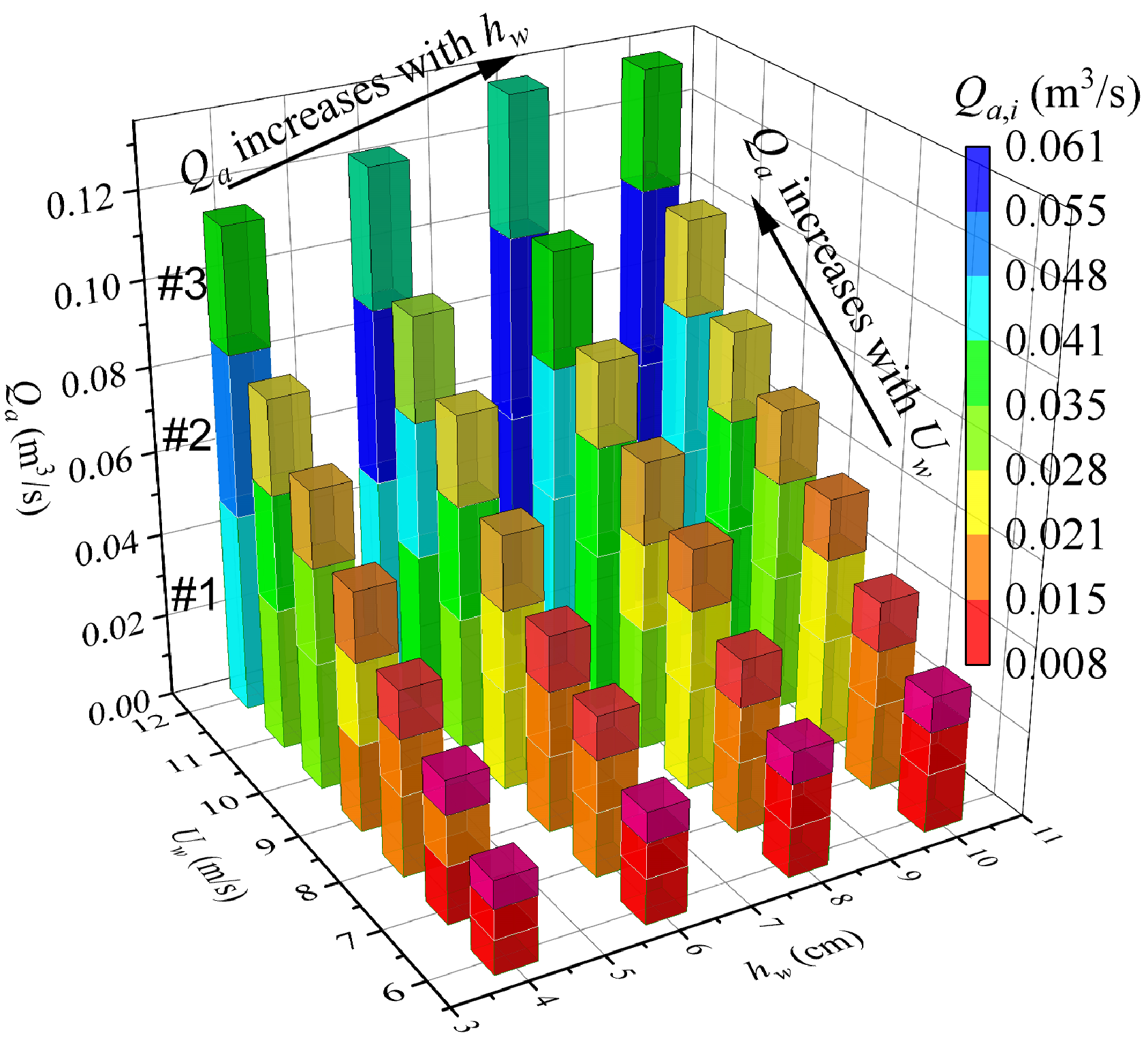
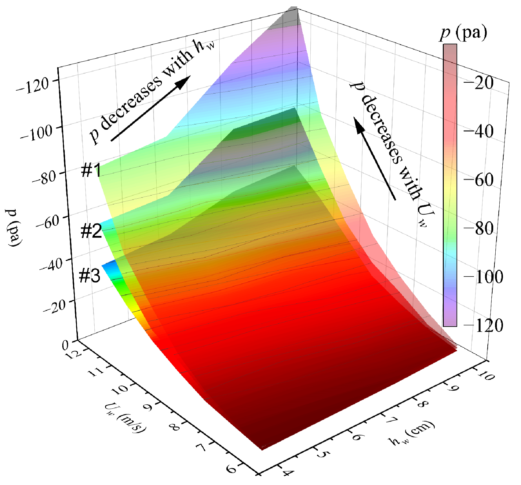
3.1. Effects of Water Velocity and Flow Depth on Air Demand

Increased pump flow elevates water velocity ( U w ), thereby increasing air discharge ( Q a ) (Figure 2). This coupling mechanism originates from two synergistic effects: (1) U w-driven air acceleration at the interface, and (2) turbulence-enhanced air entrainment. These findings align with Yue et al.’s experimental observations [23]. Increasing the flow depth leads to a reduction in the space above the free surface and an increase in the air velocity ( U A ) in the tunnel. Because the effect of increasing the air velocity on the air discharge is more significant than that of decreasing the space above the free surface at small gate openings, the air discharge increases with increasing flow depth, as shown in Figure 2. However, as the gate opening increases, the free-surface flow transforms into foamy flow [12] and the effect of increasing the air velocity becomes less significant than that of decreasing the space above the free surface, resulting in decreasing air discharge. This suggests a local peak in air discharge with a given tunnel height (h), which can be verified by prototype observations [24]. The pressure ( p i ) at the connection of the air vent and the tunnel decreases with increasing water velocity ( U w ) and water depth ( h w ) due to increasing air discharge, and the pressure ( p 1 ) closer to the gate is the lowest, as shown in Figure 3.

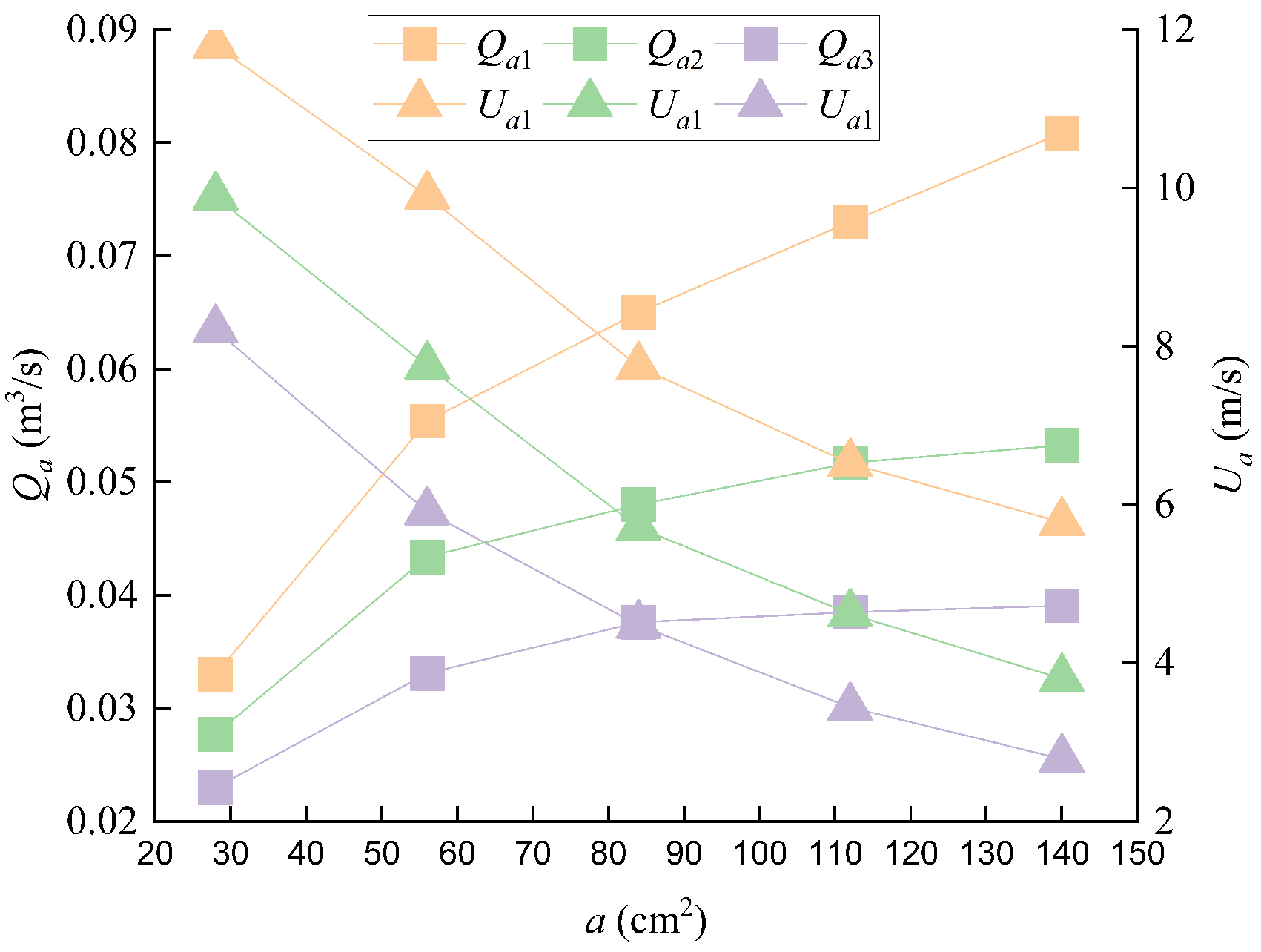
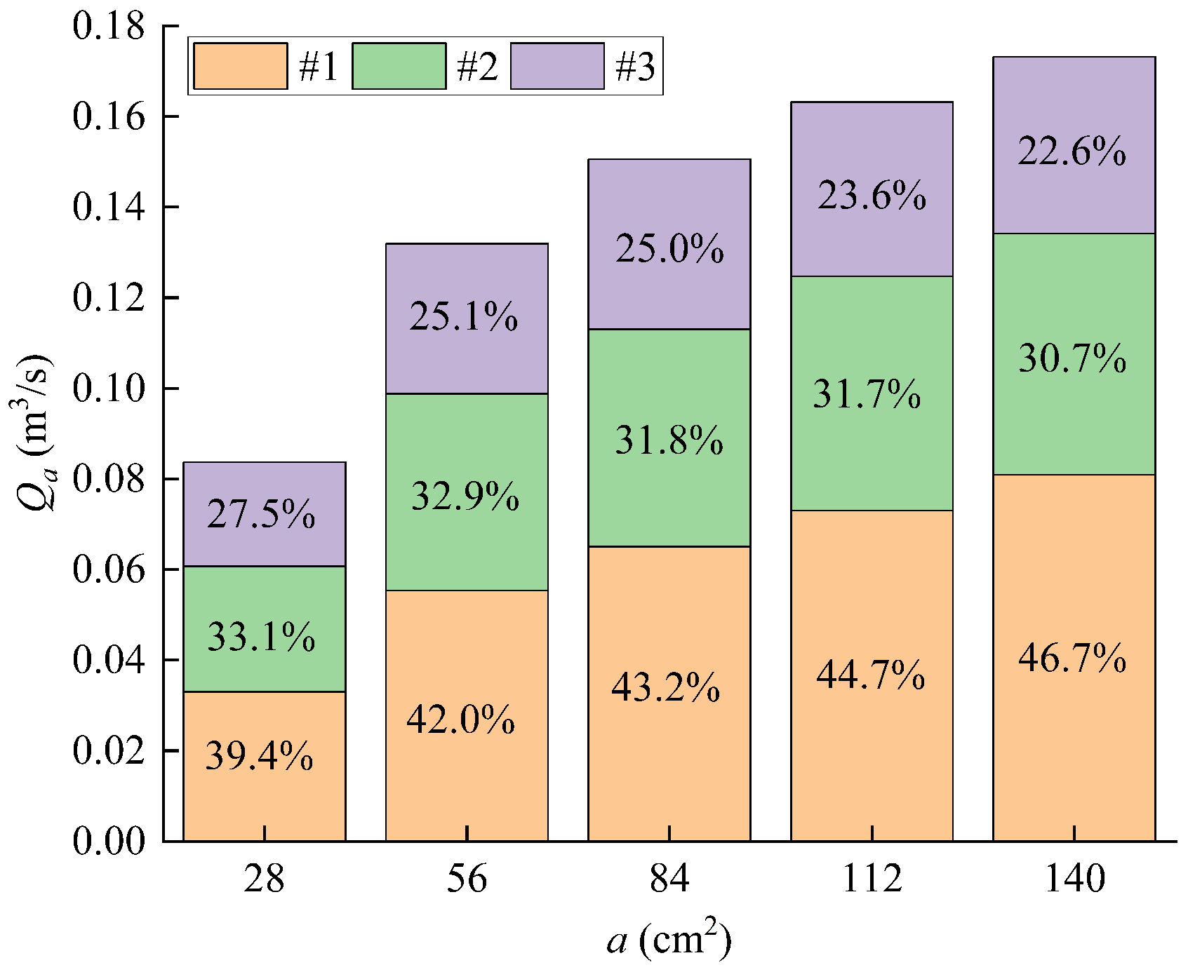
3.2. Effect of the Air Vent Area on the Air Demand

As shown in Figure 4, increasing the air vent area ( a 1 , a 2 , a 3 ) leads to increasing air discharge ( Q a ) and decreasing air velocity ( U a ), as increasing the air vent area decreases the energy loss coefficient δ of the air vent. The pressure (p) in the spillway tunnel decreases with increasing air vent area (a). The air pressure increases (from negative values towards zero) along the spillway tunnel and finally reaches atmospheric pressure at the spillway outlet, as shown in Figure 5. When the air vent connects to the tunnel, the pressure on the upstream side of the air vent is greater than that on the downstream side, which was verified by Lian’s numerical results [15]. As shown in Figure 6, the value of the air discharge ( Q a ) decreases in the order air vent #1, #2, #3 due to the decreasing pressure difference along the tunnel, and the increasing air vent area leads to an increasing percentage of air discharge in air vent #1 and a decreasing percentage of air discharge in air vents #2 and #3. Overall, it is essential to determine the optimal combination of air vent areas via the method described in Section 4.1 and to meet the air supply system requirements of spillway tunnels without causing engineering waste.

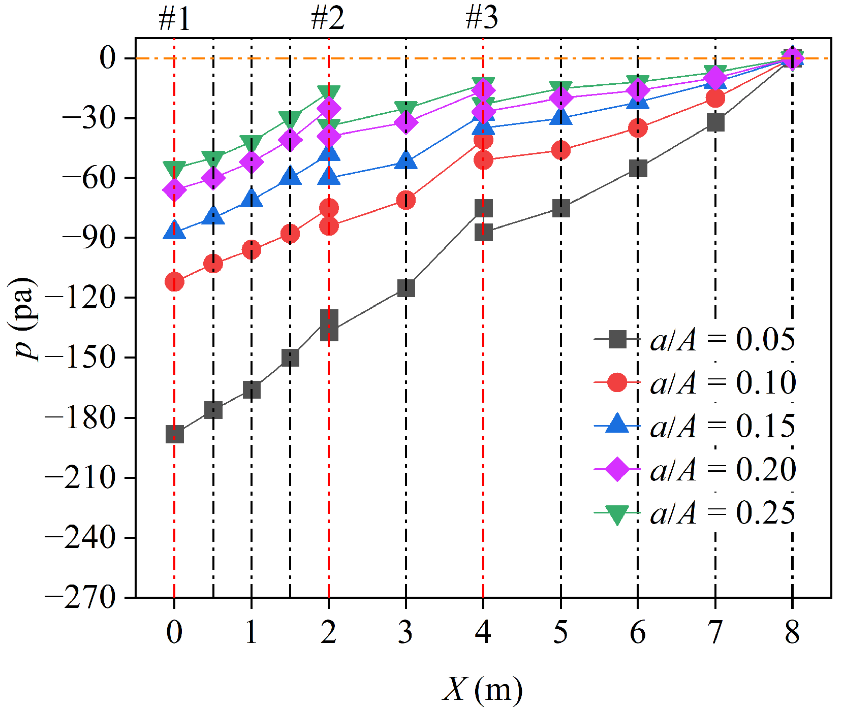
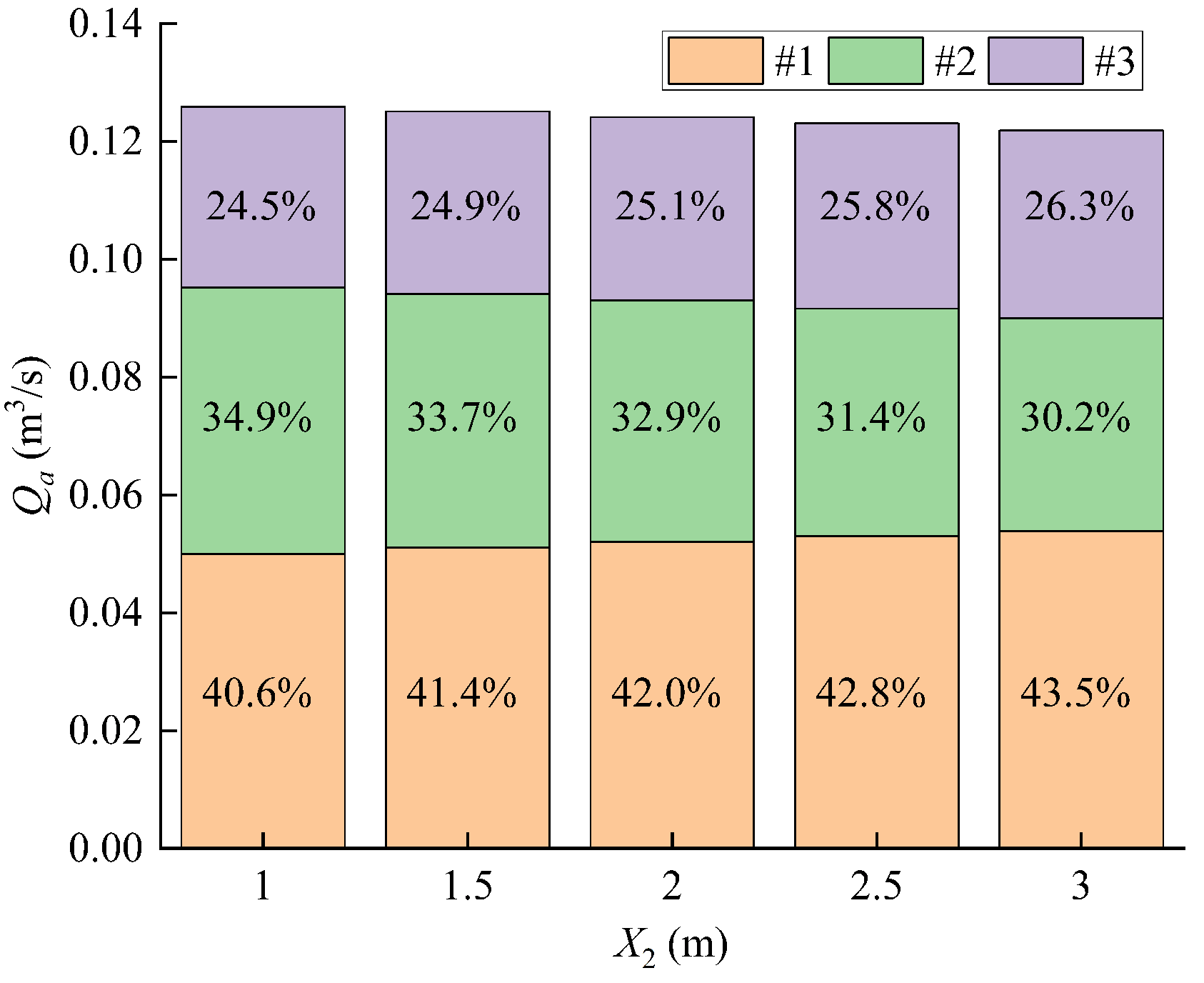
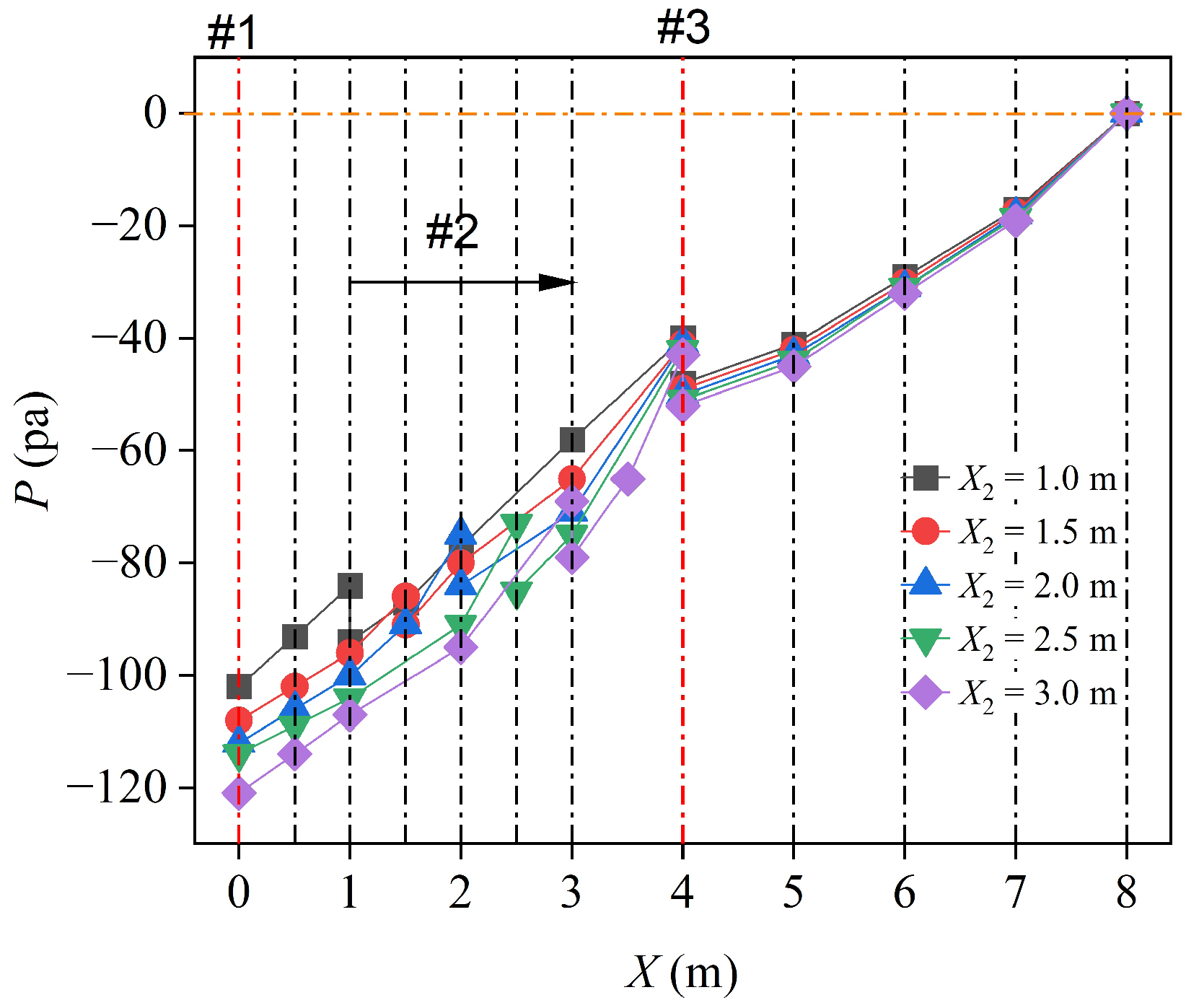
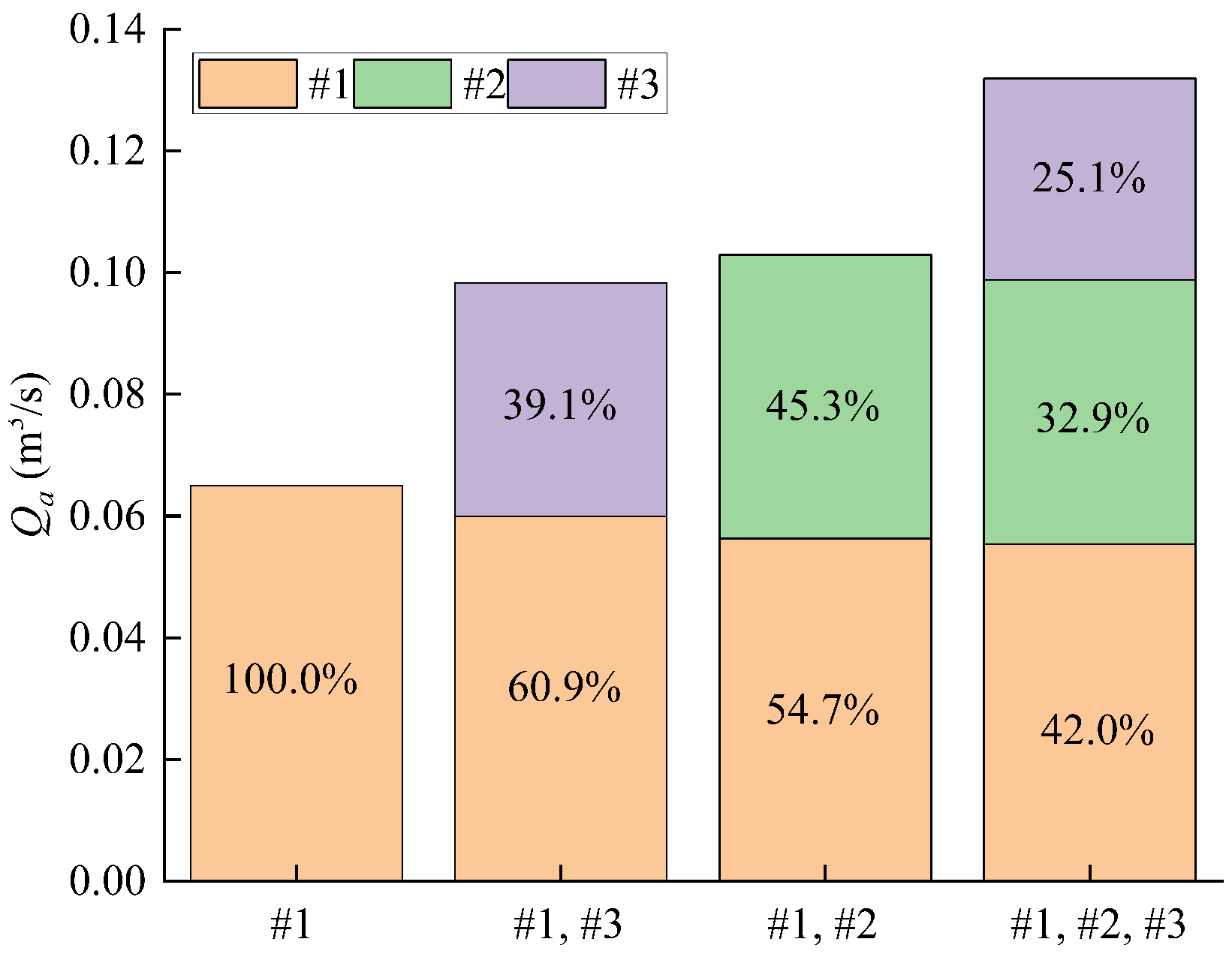
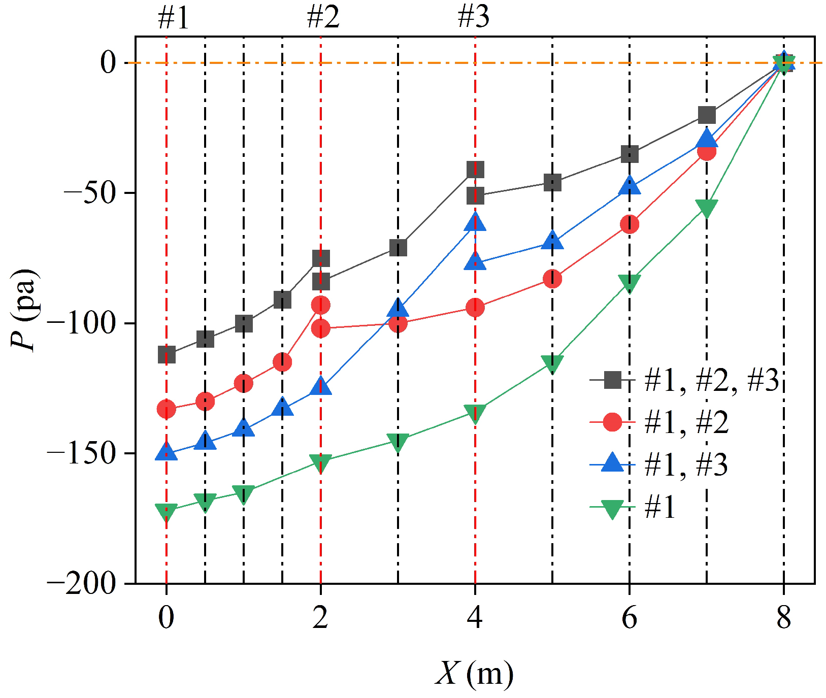
3.3. Effects of the Air Vent Location and Number on the Air Demand

As the distance ( X 2 ) from air vent #2 increases, as shown in Figure 7, the total air discharged through the air vent decreases slightly. The air discharge ( Q a , 1 ) and the percentage of air discharged from air vent #1 increase, which could be explained by the pressure in air vent #1 decreasing when air vent #2 moves downstream, as shown in Figure 8. The air discharged through air vent #3 changes only slightly because of its greater distance from the gate. Consequently, the optimal placement of air vents can improve the negative pressure distribution in the tunnel and increase the total air discharge. Considering topography, technical, and economic factors, air vents should be positioned as close to the gate as possible.
As shown in Figure 9, reducing the number of air vents decreases the total air discharge ( Q a ) through air vents and increases the air velocity ( U a , 1 ) through air vent #1. The air discharge ( Q a , 1 ) through air vent #1 in the model with air vents #1 and #3 is greater than that in the model with air vents #1 and #2, which is attributed to the greater distance of air vent #3 from the gate than that of air vent #2, resulting in a lower pressure at air vent #1 in Figure 10. The spillway tunnels with air vents #1, #2, and #3 present the lowest pressure difference and the most uniform pressure distributions along the tunnel. Therefore, the number of air vents significantly influences the air discharge of each vent. Rationally designing multiple vents for large structures with high heads can effectively increase the air discharge, reduce the air velocity, and considerably decrease the negative pressure along the spillway tunnel.

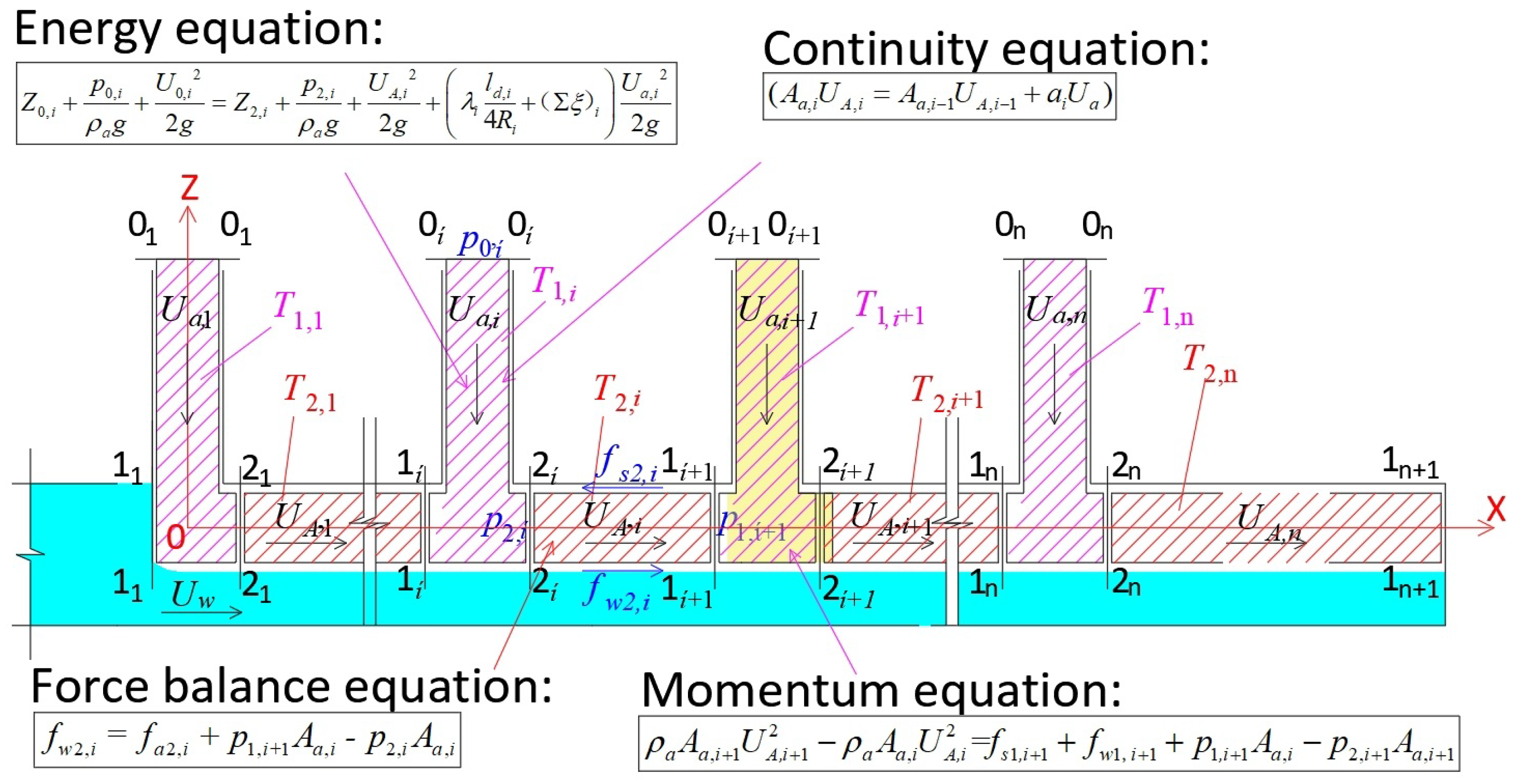
4. Calculation Equation for Air Demand

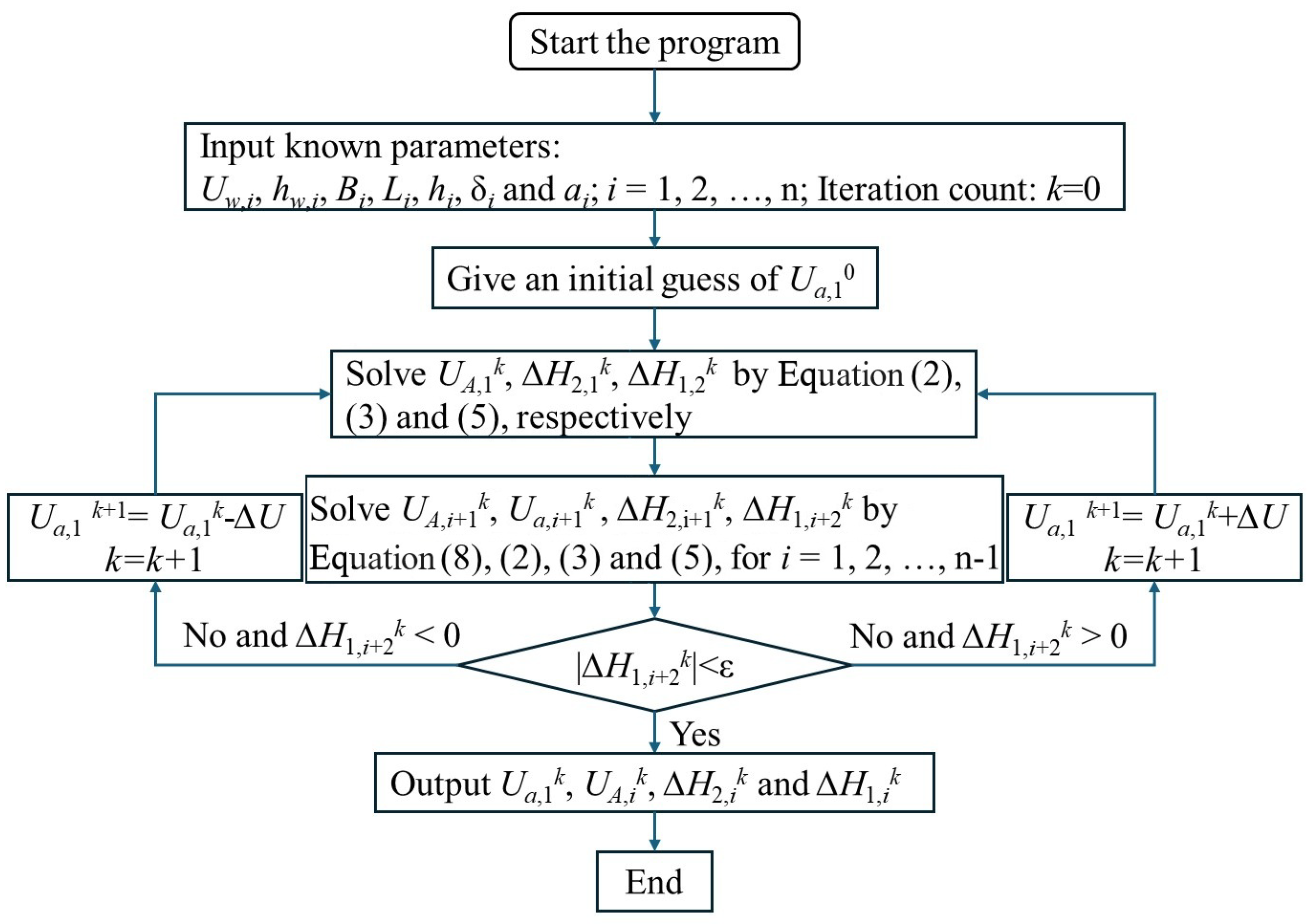
4.1. Solution Procedure for Air Demand

The above model tests reveal that hydraulic factors, such as water velocity and flow depth, and structural factors, including the air vent area and the location of air vents, significantly affect the air demand of spillway tunnels with multiple air vents. This section proposes a novel approach to calculate air discharge through air vents on the basis of energy, momentum, and force balance equations. Notably, free-surface flow is the desired flow pattern and spray flow is affected by scale and model effects. Therefore, the method was limited to free-surface flow. The air discharge value in the bubble suspension layer is approximately 10% in the air vent for free-surface flow [17]. The volume of droplets in the droplet jump layer can compensate for the volume of air in the bubble suspension layer. Thus, the air discharge in the bubble suspension layer is neglected in the derivation.
In this study, the volume of air can be divided into two main categories, as shown in Figure 11: the volume of air between section 0 i 0 i , away from each air vent inlet, and sections 1 i 1 i and 2 i 2 i serves as the control body T 1 , i + 1 , described in magenta; while the volume of air between sections 2 i 2 i and 1 i + 1 1 i + 1 serves as the control body T 2 , i , described in red.
The energy equation for the control body T 1 , i from section 0 i 0 i to 2 i 2 i is as follows:
Z 0 , i + p 0 , i ρ a g + U 0 , i 2 2 g = Z 2 , i + p 2 , i ρ a g + U A , i 2 2 g + λ i l a , i 4 R i + ( Σ ξ ) i U a , i 2 2 g
where Z 0 , i and Z 2 , i are the z-direction positions of the midpoints of sections 0 i 0 i and 2 i 2 i , respectively. The corresponding negative pressures are p 0 , i and p 2 , i , and the average air velocities are U 0 , i and U A , i . Furthermore, U a , i , l d , i , l a , i , B a , i , R i = B a , i l a , i 2 ( B a , i + l a , i ) , λ i , and ( Σ ξ ) i represent the average air velocity, length, height, width, hydraulic diameter, resistance coefficient, and the local loss coefficients of the ith air vent, respectively.
The pressure p 0 , i away from the inlet approaches atmospheric pressure, and the height difference between sections 0 i 0 i and 2 i 2 i is much smaller than the negative pressure head Δ H 2 , i = p 2 , i ρ a g , thus the height term is negligible in the derivation. U A , i can be calculated in Equation (2) by the continuity equation, and substituting δ i = λ i l d , i 4 R i + ( ξ ) i into Equation (1) yields Equation (3) for pressure head Δ H 2 , i .
U A , i A a , i = A a , i 1 U A , i 1 + a i U a , i
Δ H 2 , i = ( U A , i 2 2 g + δ i U a , i 2 2 g )
where A a i is the residual tunnel cross-sectional area above the water surface between sections 2 i 2 i and 1 i + 1 1 i + 1 , and a i is the cross-sectional area of the ith air vent; the first vent is just downstream of the gate leading to U A , 0 = 0 .
The control body T 2 , i in Figure 11 is subjected to drag force f 2 s , i at the wall, drag force f 2 w , i at the air–water interface, and negative air pressure ( p 1 , i + 1 A a , i , p 2 , i A a , i ) at sections 1 i + 1 1 i + 1 and 2 i 2 i . The drag force f 2 w , i can be expressed as f 2 w , i = τ w , i L i B i , where L i B i is the area of the air–water interface between sections 2 i 2 i and 1 i + 1 1 i + 1 . The interfacial drag stress τ w , i between air and water can be expressed as τ w , i = ρ a f i ( U w U A , i ) 2 2 , where f i is the drag coefficient given by f i = ω i B i U w 2 g A a , i . The wall drag force f 2 s , i is negligible compared to the air–water interface f 2 w , i , which aligns with the findings of Lian [15], and Equation (4) can be modified to Equation (5) to calculate Δ H 1 , i + 1 .
f 2 w , i = f 2 s , i + p 1 , i + 1 A a , i p 2 , i A a , i
Δ H 1 , i + 1 = Δ H 2 , i + ω i L i B 2 U w 2 ( U w U A , i ) 2 2 g 2 A a , i 2
where ω i is the variable coefficient of the interface drag coefficient f i .
The momentum equation in the x-direction for the control body T 1 , i + 1 can be written as
ρ a A a , i + 1 U A , i + 1 2 ρ a A a , i U A , i 2 = f 1 s , i + 1 + f 1 w , i + 1 + p 1 , i + 1 A a , i p 2 , i + 1 A a , i + 1
where f 1 s , i + 1 is the wall drag force, and f 1 w , i + 1 is the air–water interface drag force for the control body T 1 , i + 1 .
The area A a , i is larger than the area of the air–water interface for the control body T 1 , i + 1 , so the drag forces f 1 s , i + 1 , f 1 w , i + 1 can be neglected compared to air pressure forces p 1 , i + 1 A a , i , and Equation (6) is modified to Equation (7). Combining Equations (2) and (3), the average air velocity above the free surface U A , i + 1 is shown in Equation (8).
ρ a A a , i + 1 U A , i + 1 2 ρ a A a , i U A , i 2 = ρ a g Δ H 1 , i + 1 A a , i ρ a g Δ H 2 , i + 1 A a , i + 1
U A , i + 1 = E i + 1 + ( E i + 1 2 4 D i + 1 F i + 1 ) 0.5 2 D i + 1
where D i + 1 = δ i + 1 A a , i + 1 2 a i + 1 2 1 , E i + 1 = 2 δ i + 1 A a , i A a , i + 1 U A , i a i + 1 2 , and F i + 1 = ( δ i + 1 A a , i + 1 2 a i + 1 2 + 2 A a , i A a , i + 1 ) U A , i 2 + 2 g A a , i Δ H 1 , i A a , i + 1 .
The flow diagram of the procedure can be seen in Figure 12, in which the superscript k denotes the variables solved in the kth iteration; Δ U is a slight change in the variables, which is set to be 1 × 10 4 U a , 1 k ; and ϵ is the tolerance for convergence, which is set to be 1 × 10 4 Δ H 2 , 1 k for this study.

4.2. Analysis of the Interfacial Shear Stress Formulation

Previous studies have indicated that the variation coefficient ( ω ) in Equation (5) can be expressed as a function of the air–water interface amplitude, which is related to the root mean square of the normal fluctuating velocity ( [ ν 2 ¯ ] 0.5 ) near the air–water interface [13,14,25]. A study of uniform open-channel flow revealed that the mean normal pulsating velocity ( [ ν 2 ¯ ] 0.5 ) and friction velocity ( u * ) satisfies Equation (9) [26,27], and Equation (10) can be derived from the force balance equation [26]. [ ν 2 ¯ ] 0.5 can be calculated from the hydraulic radius (R) and hydraulic slope (J), as shown in Equation (11).
( [ ν 2 ¯ ] 0.5 u * ) Z = h w = 1.48 e 0.7
u * = ( g R J ) 0.5
[ ν 2 ¯ ] 0.5 = 1.48 × e 0.7 × u * = 0.735 u * = 0.735 ( g R J ) 0.5
Combining Chézy’s formula, Manning’s formula, and Manning’s coefficient formula in Equation (12), ( R J ) 0.5 can be calculated in Equation (13) [28].
( R J ) 0.5 = U w C C = R 1 / 6 n n = 0.038 R 1 / 6 ( 17 μ w ρ w U w R + 0.25 Δ R ) 0.125
( R J ) 0.5 = 0.038 ( 17 μ w ρ w U w R + 0.25 Δ R ) 0.125 U w
Equations (11) and (13) show that the inverted roughness ( Δ ) has a strong effect on the normal fluctuating velocity ( [ ν 2 ¯ ] 0.5 ), which can be explained by the fact that roughening of the invert can break the laminar sublayer and increase the surface turbulence intensity [28,29,30,31,32]. Thus, the relationship in Equation (14) can be rationally assumed for the free-surface flow pattern.
ω [ ν 2 ¯ ] 0.5 g 0.5 ( 17 μ w ρ w U w R + 0.25 Δ R ) 0.125 U w
On the basis of the model test data of case (5), the variation coefficient ( ω 0 ) was calculated via the method described in Section 4.1, combining the loss coefficient ( δ i ) of the ith vent computed via Equation (15) [33]. The optimal fit (Equation (16), Figure 13) was obtained through linear least-squares regression, yielding a mean absolute percentage error (MAPE) of 6.95% across the experimental dataset. The relationship demonstrates strong predictive accuracy (R2 = 0.937) with 95% confidence bounds of the regression coefficient. This statistical validation aligns with established methodologies for hydraulic parameter estimation [34].
δ i = λ i s i d i + ξ i 0.015 × 16 + 1.8 = 2.04
ω = 1.3648 × 10 5 g 0.5 ( 17 μ w ρ w U w R + 0.25 Δ R ) 0.125 U w

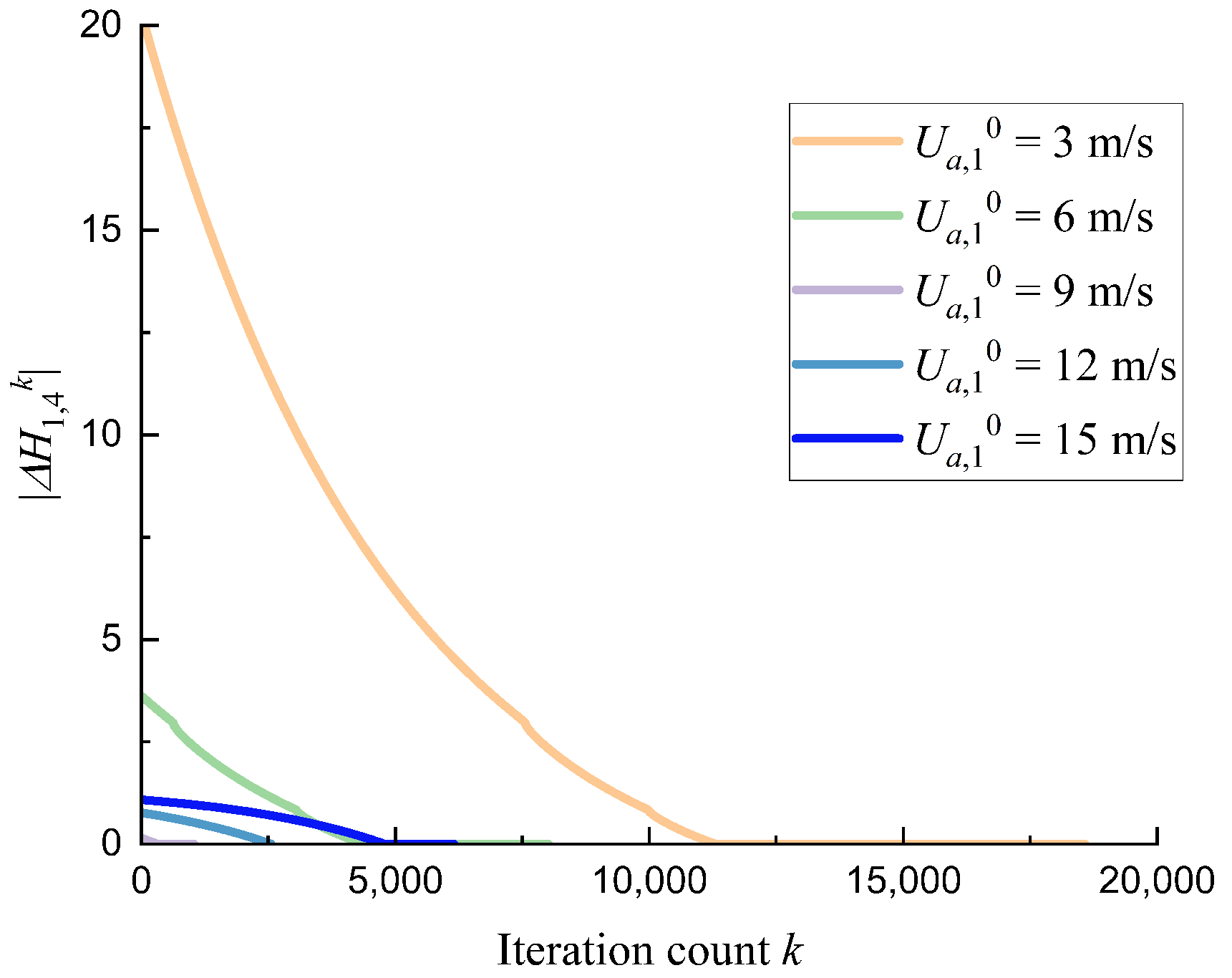
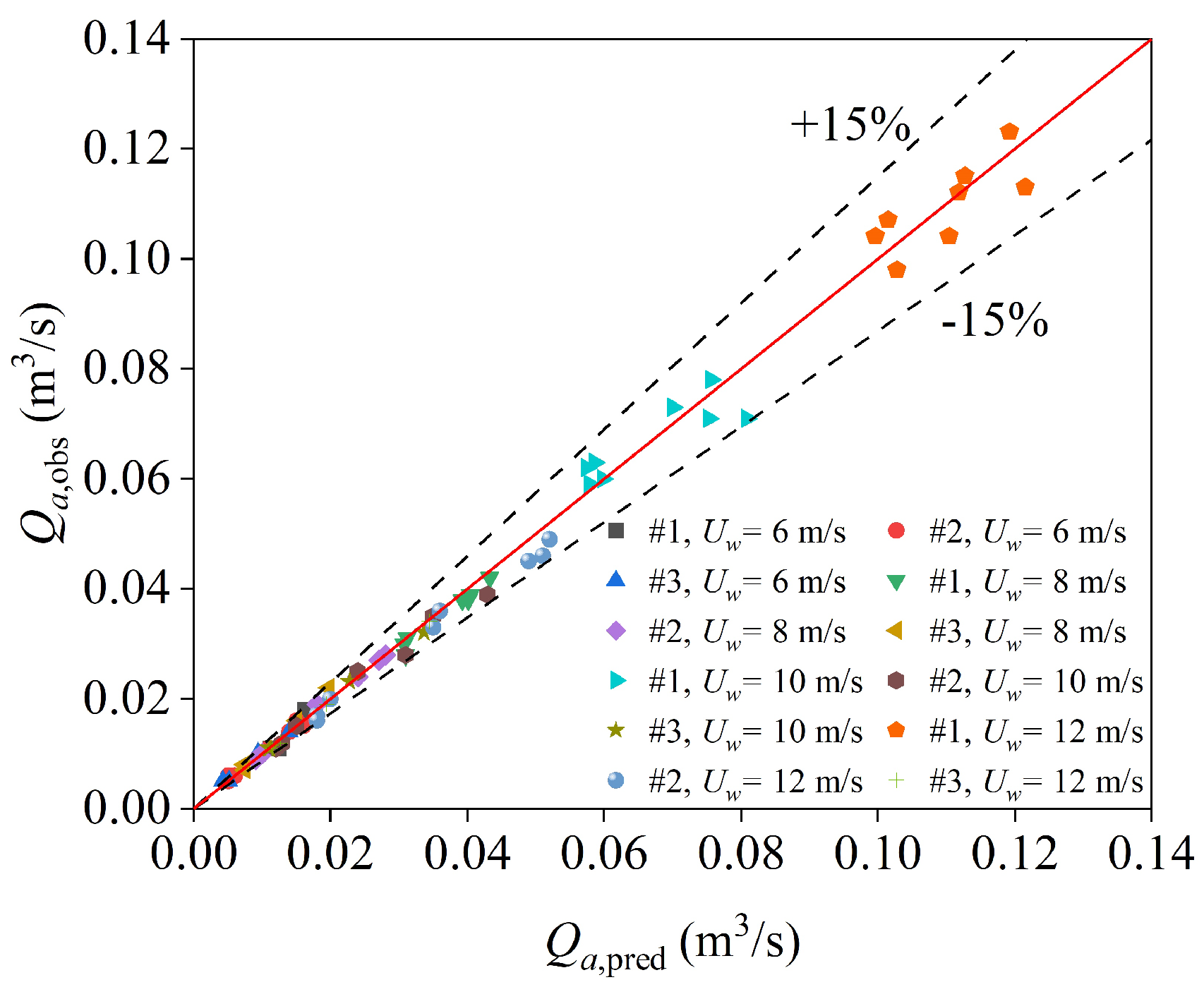
4.3. Convergence and Sensitivity Analysis

The relationship between inverted roughness and the interfacial drag coefficient established in Section 4.2 was incorporated into the model described in Section 4.1 to predict the air velocities through multiple vents. Due to the inherent nonlinear interactions among the system variables, analytical derivation of the convergence properties and sensitivity coefficients through conventional theoretical methods proved impractical. To address this limitation, we implemented a parametric sensitivity analysis by perturbing five key operational parameters—water velocity, water depth, total loss coefficients of vents, inverted roughness, and tunnel length—from baseline conditions ( a 1 = a 2 = a 3 = 56 cm 2 , U w = 12 m / s , h w = 0.08 m , L 1 = L 2 = 2 m , L 3 = 4 m ). The resultant sensitivity characteristics are quantitatively summarized in Table 3. We assigned five distinct initial air velocities ( U a , 1 0 ) and analyzed their numerical residuals for the semi-iterative loop (see Figure 14).
Parameter variations exert the strongest influence on vent 1#, with vents 2# and 3# exhibiting decreasing sensitivity. Water velocity emerges as the dominant control parameter, where a 10% increase causes a 21.94% rise in air velocity through vent 1#. A comparative analysis reveals that 10% perturbations in water depth, total loss coefficients of vents, inverted roughness, and tunnel length induce minimal effects, producing less than 3.5% variation in air velocity. These findings emphasize the critical importance of high-accuracy water velocity measurements for operational modeling. A convergence efficiency analysis showed that initial values closer to the final solution required fewer iterations, with the maximum computational time in MATLAB 2023b remaining below 1.26 s—demonstrating sufficient efficiency for preliminary design applications.

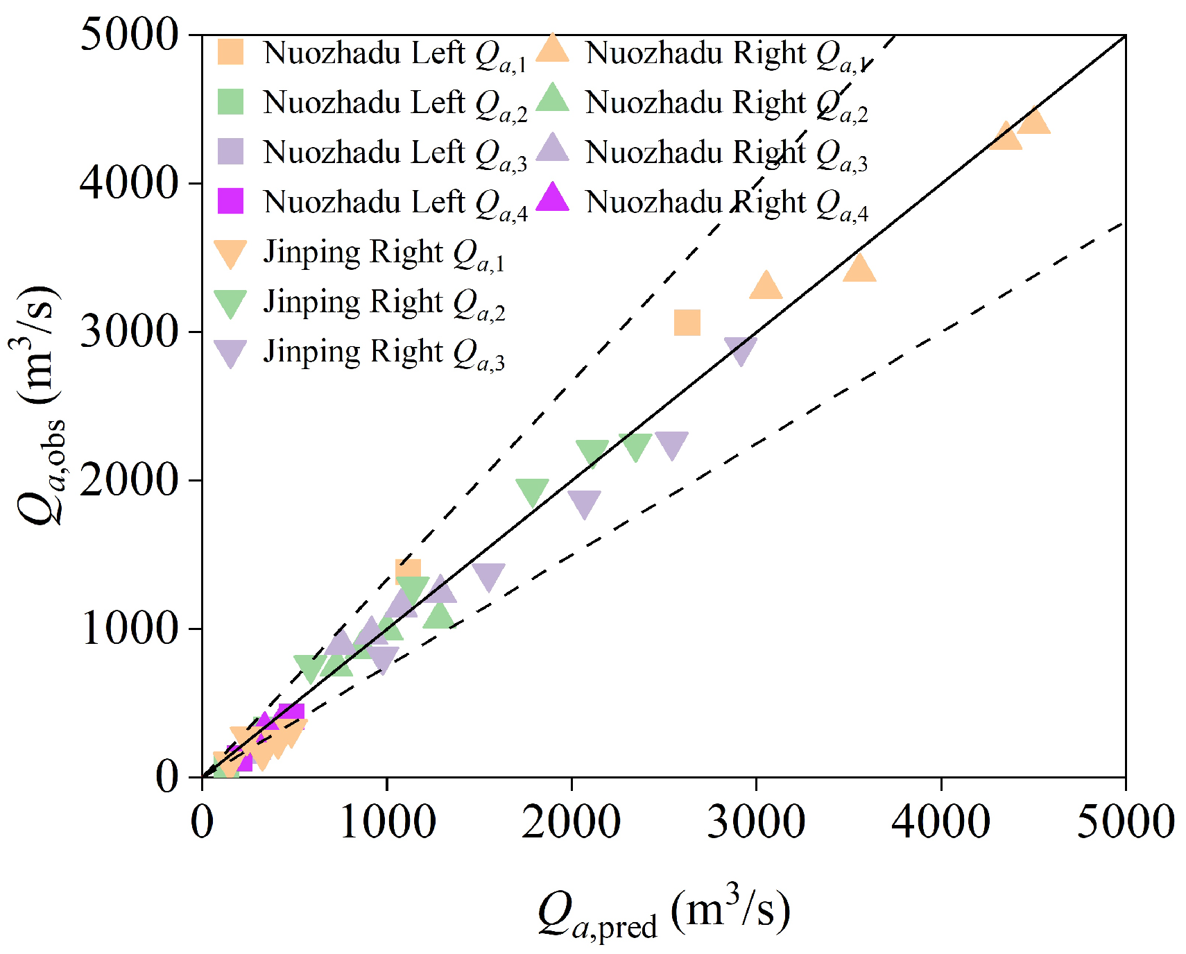
4.4. Comparison of the Prototype and Model Test Dates

This section details the practical implementation of the proposed air demand calculation equation. The validation efforts faced inherent challenges arising from two primary limitations: (1) The spillway tunnel’s multi-vent configuration, and (2) the method’s sensitivity to precise flow characteristics. These constraints, combined with the methodology’s restriction to free-surface flow conditions, complicated parameter identification. To address these challenges, the required parameters were taken from two literature datasets (cataloged in Table 4): Nuozhadu Dam [35] and Jinping-I Dam [36]. The calculation equation was further applied to four model test cases (cases (1)–(4)), with the computational results illustrated in Figure 15.
The model test Froude numbers (Fr < 19) align with prototype observation ranges (Fr < 8), where air entrainment and scale effects are negligible in free-surface flow [1,37,38]. This alignment validates the Section 4.2 model for comparing observed prototype air demand ( Q a , obs ) with predictions, as shown in Figure 16. For prototype data from the Nuozhadu and Jinping-I projects, the predictions closely follow the 45° equivalence line, exhibiting a mean absolute percentage error (MAPE) of 19.95% and R 2 = 0.980, with all data trends captured within a ±25% deviation range. The model experiments (cases (1)–(4)) demonstrate even stronger agreement, yielding an MAPE of 4.38% and R 2 = 0.993, with deviations confined to ±15%. These results confirm robust consistency between the spillway tunnel air demand predictions and both the prototype and experimental measurements.
The solution for the air demand of spillway tunnels in free-surface flow presented in this paper comprehensively includes the main hydraulic factors and structural factors on the basis of the interfacial shear stress formulation and can be considered a preliminary design method. For practical applications, more prototype data, such as wall roughness and the location of air vents, are needed to quantify the contributions of different effects in more detail.

5. Conclusions

This study identifies critical factors governing air demand in spillway tunnels under free-surface flow conditions ( Fr < 19 ): Air discharge correlates positively with (1) flow velocity, (2) relative flow depth (at constant tunnel height), and (3) air vent area and quantity. A novel design framework integrating energy–momentum equations, force balance principles, and experimental interfacial shear stress formulations was developed to optimize vent configuration. The hydraulic design of ventilation systems should prioritize limiting vent airspeed, with a recommended maximum allowable velocity of 60 m/s. If this criterion is unmet, structural adjustments—such as increasing vent area or quantity, or optimizing proximal gate placement—or operational modifications—such as reducing flow velocity or gate opening—can effectively constrain the airspeed. Notably, the model’s validity under non-free-surface flow regimes (e.g., pressurized or transitional flows) and complex geometries remains unvalidated and requires further study. Future research should prioritize three objectives: (1) more comprehensive prototypic condition validation to evaluate scale effects, and (2) extension to high-Froude-number flows ( Fr > 19 ) and mixed-regime scenarios. These advancements will strengthen the robustness of air demand predictions for real-world spillway designs while addressing the study’s limitations.

Author Contributions

Conceptualization, H.Y. and W.W.; data curation, Q.F.; formal analysis, H.Y., W.W., and Z.T.; funding acquisition, Z.T.; investigation, H.Y.; methodology, H.Y.; project administration, Z.T.; resources, Z.T.; software, H.Y.; supervision, W.W.; validation, Q.F.; visualization, H.Y.; writing—original draft, H.Y.; writing—review and editing, Z.T. All authors have read and agreed to the published version of the manuscript.

Funding

This work was supported by the National Natural Science Foundation of China [51879178].

Institutional Review Board Statement

Not applicable.

Informed Consent Statement

Not applicable.

Data Availability Statement

The original contributions presented in the study are included in the article. Further inquiries can be directed to the corresponding author.

Conflicts of Interest

The authors declare no conflicts of interest.

References

  1. Pagliara, S.; Hohermuth, B.; Boes, R.M. Air–Water Flow Patterns and Shockwave Formation in Low-Level Outlets. J. Hydraul. Eng. 2023, 149, 06023002. [Google Scholar] [CrossRef]
  2. Speerli, J.; Hager, W.H. Air-water flow in bottom outlets. Can. J. Civ. Eng. 2000, 27, 454–462. [Google Scholar] [CrossRef]
  3. Gao, Y.; Xu, H. Experimental study on pressurized and free-surface flow of discharge tunnel. J. Hydraul. Eng. 1964, 4, 52–57. [Google Scholar] [CrossRef]
  4. Crookston, B.M.; Erpicum, S. Hydraulic engineering of dams. J. Hydraul. Res. 2022, 60, 184–186. [Google Scholar] [CrossRef]
  5. Falvey, H.T. Air-water flow in hydraulic structures. NASA STI/Recon Tech. Rep. N 1980, 81, 26429. [Google Scholar]
  6. Hohermuth, B.; Vetsch, D.F.; Schmocker, L.; Felder, S.; Boes, R.M. Air-Water Flow Downstream of High-Head Sluice Gates: Experimental and Numerical Investigations. In Proceedings of the 38th IAHR World Congress—Water: Connecting the World, Panama City, Panama, 1–6 September 2019. [Google Scholar]
  7. Wei, W.R.; Deng, J.; Xu, W. Numerical investigation of air demand by the free surface tunnel flows. J. Hydraul. Res. 2021, 59, 158–165. [Google Scholar] [CrossRef]
  8. Kalinske, A.A.; Robertson, J.M. Entrainment of Air in Flowing Water: A Symposium: Closed Conduit Flow. Trans. Am. Soc. Civ. Eng. 1943, 108, 1435–1447. [Google Scholar] [CrossRef]
  9. Campbell, F.; Guyton, B. Air Demand In Gated Outlet Works. In Proceedings of the Minnesota International Hydraulic Convention, Minneapolis, MN, USA, 1–4 September 1953; pp. 529–533. [Google Scholar]
  10. Wisner, P. Hydraulic design for flood control by high head gated outlets. In Proceedings of the 9th ICOLD Congress, Istanbul, Turkey, 4–8 September 1967; pp. 495–507. [Google Scholar]
  11. Sharma, H.R. Air Demand for High Head Gated Conduits. Ph.D. Thesis, Norwegian Institute of Technology, University of Trondheim, Trondheim, Norway, 1973. [Google Scholar]
  12. Hohermuth, B.; Schmocker, L.; Boes, R.M. Air Demand of Low-Level Outlets for Large Dams. J. Hydraul. Eng. 2020, 146, 04020055. [Google Scholar] [CrossRef]
  13. Gao, Y. Ventilation of closed drain pipes. In Progress in Water Conservancy and Hydropower Science and Technology; Water Resources Press: Beijing, China, 1963; Volume 1, pp. 138–148. [Google Scholar]
  14. Luo, H. Study of air intake problems in drainage pipes. J. Hydraul. Eng. 1984, 64–70. [Google Scholar]
  15. Lian, J.; Wang, X.; Liu, D. Air demand prediction and air duct design optimization method for spillway tunnel. J. Hydraul. Res. 2021, 59, 448–461. [Google Scholar] [CrossRef]
  16. Wang, X.; Lian, J. Numerical Investigation on Air–Water Two-Phase Flow of Jinping-I Spillway Tunnel. Appl. Sci. 2022, 12, 4311. [Google Scholar] [CrossRef]
  17. Yazdi, J.; Zarrati, A.R. An algorithm for calculating air demand in gated tunnels using a 3D numerical model. J. Hydro-Environ. Res. 2011, 5, 3–13. [Google Scholar] [CrossRef]
  18. Fan, W.; Anglart, H. A new set of volume of fluid solvers for turbulent isothermal multiphase flows in OpenFOAM. Comput. Phys. Commun. 2020, 247, 106876. [Google Scholar] [CrossRef]
  19. Almeland, S.K.; Mukha, T.; Bensow, R.E. An improved air entrainment model for stepped spillways. Appl. Math. Model. 2021, 100, 170–191. [Google Scholar] [CrossRef]
  20. Bertolotti, L.; Jefferson Loveday, R.; Ambrose, S.; Korsukova, E. A comparison of volume of fluid and Euler–Euler approaches in computational fluid dynamics modeling of two-phase flows with a sharp interface. J. Turbomach. 2021, 143, 121005. [Google Scholar] [CrossRef]
  21. Zhang, H.Q.; Zhang, X.T.; Lou, Y.L.; Xing, W.P. Comparative Analysis of Wind Speed in Ventilation Hole Simulated by VOF and Euler Model. Appl. Mech. Mater. 2014, 624, 643–646. [Google Scholar] [CrossRef]
  22. González, F.S.; Saiz, J.S.M.; Jordana, M.Á.C.; de Navarra, E.O.I. Air demand estimation in bottom outlets with the particle finite element method. Susqueda Dam case study. Comput. Part. Mech. 2017, 4, 345–356. [Google Scholar]
  23. Yue, S.; Diao, M.; Zhao, J. Analysis and Research of Aeration Capacity of the Spillway Tunnel with High Speed Flows. Adv. Eng. Sci. 2013, 45, 7–12. [Google Scholar] [CrossRef]
  24. Chen, Z.; Huang, W.; Ye, S. A study of prototype law of air demand in flood control conduits. Hydro-Sci. Eng. 1986, 1, 1–18. [Google Scholar] [CrossRef]
  25. Wang, W.; Liao, W.; Qi, L. Experiment of turbulent characteristics of flow in wide-and-narrow channels. Adv. Water Sci. 2020, 31, 394–403. [Google Scholar] [CrossRef]
  26. Liu, C.; Li, D.; Wang, X. Experimental study on friction velocity and velocity profile of open channel flow. J. Hydraul. Eng. 2005, 8, 950–955. [Google Scholar]
  27. Nezu, I.; Rodi, W. Open-channel Flow Measurements with a Laser Doppler Anemometer. J. Hydraul. Eng. 1986, 112, 335–355. [Google Scholar] [CrossRef]
  28. Yang, C. Research of Roughness Coefficient and Turbulence Character in Uniform Flow of Open Channel. Master’s Thesis, Northwest A&F University, Xianyang, China, 2010. [Google Scholar]
  29. Liu, D. Hydraulic Modelling of Air Demand of Aerators on High Velocity Sluicing Structures. J. Change River Sci. Res. Inst. 1995, 1, 1–10. [Google Scholar]
  30. Lv, H.; Yu, J. Experimental Research on Sudden Rising of Wall Roughness in Open Channels on the Effect of Turbulent Velocity and Turbulence Intensity. China Rural. Water Hydropower 2011, 1, 97–99. [Google Scholar]
  31. Ramesh, B.; Kothyari, U.C. Turbulence characteristics in an open channel flow over transitionally rough bed. ISH J. Hydraul. Eng. 2014, 20, 169–176. [Google Scholar] [CrossRef]
  32. Zhong, L.; Jiang, T.; Zhang, J.; Liu, J. PIV Experimental Study on Velocity Fluctuations of Turbulent Flow in Open Channel. Adv. Eng. Sci. 2019, 51, 84–93. [Google Scholar] [CrossRef]
  33. Brater, E.F.; King, H.W.; Lindell, J.E.; Wei, C.Y. Handbook of Hydraulics for the Solution of Hydraulic Engineering Problems, 7th ed.; McGraw-Hill Professional: New York, NY, USA, 1996. [Google Scholar]
  34. Yoosefdoost, A.; Lubitz, W.D. Sluice Gate Design and Calibration: Simplified Models to Distinguish Flow Conditions and Estimate Discharge Coefficient and Flow Rate. Water 2022, 14, 1215. [Google Scholar] [CrossRef]
  35. Zheng, D.; Chen, Y. Report on the Study of Ventilation and Noise Reduction in the Spillway Tunnel of Yunnan Lancangjiang River Nuozhadu Hydropower Project; Technical Report 1; Kunming Engineering Corporation Limited: Kunming, China, 2015. [Google Scholar]
  36. Lian, J.; Qi, C.; Liu, F.; Gou, W.; Pan, S.; Ouyang, Q. Air Entrainment and Air Demand in the Spillway Tunnel at the Jinping-I Dam. Appl. Sci. 2017, 7, 930. [Google Scholar] [CrossRef]
  37. Rabben, S.; Rouve, G. Air demand of high head gates-model-family studies to quantify scale effects. In Proceedings of the IAHR Symposium on Scale Effects in Modelling Hydraulic Structures, Esslingen am Neckar, Germany, 3–6 September 1984; pp. 4–9. [Google Scholar]
  38. Rabben, S. Untersuchung der Belüftung an Tiefschützen Unter besonderer Berücksichtigung von Maßstabseffekten. Ph.D. Thesis, Institut für Wasserbau und Wasserwirtschaft, Rheinisch-Westfälische Technische Hochschule Aachen, Aachen, Germany, 1984. Available online: https://publications.rwth-aachen.de/record/68562 (accessed on 1 May 2025).
Figure 1. Schematic of spillway tunnel physical model at SKLH: (a) Panoramic view. (b) Front view. (c) Top view.
Applsci 15 05831 g001
Figure 2. Air demand ( Q a , i ) of the air vent versus water velocity ( U w ) and water depth ( h w ).
Applsci 15 05831 g002
Figure 3. Air pressure p at the connection of the air vent and the tunnel under varying water flow conditions ( U w and h w ).
Applsci 15 05831 g003
Figure 4. Functional relationships between air flow characteristics ( U a , Q a ) and air vent area (a).
Applsci 15 05831 g004
Figure 5. Relative air pressure distribution (p) along the tunnel for different air vent areas.
Applsci 15 05831 g005
Figure 6. Percentage of the total air discharge along the tunnel as a function of air vent area (a).
Applsci 15 05831 g006
Figure 7. Percentage of the total air discharge as a function of the location ( X 2 ) of air vent #2.
Applsci 15 05831 g007
Figure 8. Relative air pressure distribution along the tunnel as a function of the location ( X 2 ) of air vent #2.
Applsci 15 05831 g008
Figure 9. Percentage of the total air discharge with different number of air vents.
Applsci 15 05831 g009
Figure 10. Relative air pressure distribution along the tunnel for different number of air vents.
Applsci 15 05831 g010
Figure 11. Schematic diagram of air–water stratified flow.
Applsci 15 05831 g011
Figure 12. Flow diagram of the solution procedure for air demand.
Applsci 15 05831 g012
Figure 13. The variation coefficient ( ω ) as a function of g 0.5 ( 17 μ w ρ w U w R + 0.25 Δ R ) 0.125 U w ; data for case (5).
Applsci 15 05831 g013
Figure 14. Residual evolution vs. iteration count (k) for five air velocity ( U a , 1 0 ) initializations.
Applsci 15 05831 g014
Figure 15. Comparison of air demand: experimental measurements data ( Q a , obs ) versus predicted data ( Q a , pred ); dashed lines = ± 15%.
Applsci 15 05831 g015
Figure 16. Comparison of air demand: prototype data ( Q a , obs ) versus predicted data ( Q a , pred ); dashed lines = ±25%.
Applsci 15 05831 g016
Table 1. Overview of existing air demand ( Q a ) equations for spillway tunnel.
ReferenceEquationFlow Pattern
Kalinske [8] Q a = 0.0066 ( Fr o 1 ) 1.4 Q w Hydraulic jump
Campbell [9] Q a = 0.04 ( Fr c 1 ) 0.85 Q w Free-surface flow
Wisner [10] Q a = 0.040 ( Fr c 1 ) 0.85 Q w Hydraulic jump
Q a = 0.014 ( Fr c 1 ) 1.4 Q w Hydraulic jump
Q a = 0.024 ( Fr c 1 ) 1.4 Q w Free-surface flow
Sharma [11] Q a = 0.0066 ( Fr c 1 ) 0.85 Q w Free-surface flow
Q a = 0.0066 ( Fr c 1 ) 0.85 Q w Hydraulic jump
Speerli [2] Q a = 0.022 H E δ 0.43 L h 0.167 h o h o max 0.5 g B 3 0.5 Free-surface flow
Hohermuth [12] Q a = 0.037 Fr c 1.3 ( a A ( δ + 1 ) 0.5 ) 0.8 ( L h ) 0.25 ( 1 + S ) 1.5 Q w Free-surface flow
Gao [13] Q a = U w A a 1 + δ A a / ( f L B ) 0.5 A a / a with f = 2 ( 5.85 lg ( ( 2 h w + B ) h a B h w S + 1 ) 1.76 ) 2 Free-surface flow
Luo [14] Q a = U w A a 1 + δ A a / ( f L B ) 0.5 A a / a with f = B U w 2 450 g A a Free-surface flow
Lian [15] Q a = U w A a 1 + δ A a / ( f L B ) 0.5 A a / a with f = ω U w 2 ( h h w ) g 2 Free-surface flow
Fr o = U w / g h o ; where U w = average water velocity, g = gravitational acceleration, h o = gate opening. Fr c = U w / g h c ; where h c = water depth at the vena contracta section. Q w = average water discharge. H E = total energy head at the gate. δ = variable loss coefficient of the air vent. a = cross-sectional area of the air vent. L = tunnel length. h = tunnel clearance height. h o m a x = maximum allowable gate opening. A = cross-sectional area of the tunnel. S = tunnel bed slope. A a = cross-sectional area of airspace above the free surface. f = air–water interfacial drag coefficient. h a = airspace height above the free surface. h w = flow depth in the water section. ω = correction factor for the interfacial drag coefficient f.
Table 2. Summary of hydraulic model tests under free-surface flow conditions (Fr < 19).
CaseCondition 1Condition 2Comment
(1) U w = 6, 7, 8, 9, 10, 11, 12 m/s h w = 4, 6, 8, 10 cm a 1 = a 2 = a 3 = 56 cm 2
L 1 = L 2 = 2 m, L 3 = 4 m
(2) a 1 = a 2 = a 3 = 28 , 56 , 84 , 112 , 140 cm 2 L 1 = L 2 = 2 m, U w = 12 m/s, h w = 8 cm
L 3 = 4 m
(3) a 1 = a 2 = a 3 = 56  cm 2 L 1 , L 2 , L 3 = U w = 12 m/s, h w = 8  cm
1.0 , 3.0 , 4.0 m;
1.5 , 2.5 , 4.0 m;
2.0 , 2.0 , 4.0  m;
2.5 , 1.5 , 4.0  m;
3.0 , 1.0 , 4.0  m
(4) a 1 = a 2 = a 3 = 56  cm 2 L 1 , L 2 , L 3 = U w = 12  m/s, h w = 8  cm
8.0 , ,  m;
4.0 , 4.0 ,  m;
2.0 , 6.0 ,  m;
2.0 , 2.0 , 4.0  m
(5) U w = 6 , 8 , 10 , 12 m/s Δ = 12, 45, 60, 70, 110, 180, 240 μ m a 1 = 56  cm 2 , h w = 8  cm,
L 1 = 8 m
Table 3. Parametric sensitivity analysis of effects of hydraulic and structural variables on air velocity in multiple vents.
% Δ U w / U w Δ h w / h w Δ δ / δ Δ Δ / Δ Δ L 1 / L 1
−10−5510−10−5510−10−5510−10−5510−10−5510
Δ U a 1 / U a 1 −19.97−10.2410.7321.94−3.38−1.691.673.313.321.61−1.52−2.97−0.32−0.160.150.30−1.72−0.861.680.85
Δ U a 2 / U a 2 −18.95−9.6610.0120.33−1.73−0.790.600.952.691.32−1.26−2.47−0.29−0.140.140.270.440.22−0.43−0.21
Δ U a 3 / U a 3 −18.14−9.209.4419.07−0.38−0.05−0.29−1.012.151.06−1.03−2.04−0.25−0.130.120.240.490.24−0.48−0.24
Table 4. Prototype observations on the Nuozhadu Dam and the Jinping-I Dam (Fr < 8.0).
ProjectSpillway TunnelAir Vent Area ( m 2 ) H w  (m) U w  (m) U a (m/s)
B  (m) h  (m) L  (m) a 1 a 2 a 3 a 4 #1#2#3#4
Nuozhadu
Left
1216497.83189.6121.735.644.710.818.810.8
9.034.898.840.621.732.5
Nuozhadu
Right
1216.5382.7369.429.429.423.436.591.479.094.510.8
5.136.494.592.0101.715.3
6.836.2119.3105.1121.715.3
8.536.1122.2113.7131.515.3
JinPing-I
Right
13171407853636/1.122.019.523.822.6/
3.518.832.244.038.2
7.017.446.754.051.8
10.516.961.161.362.8
14.019.052.262.580.4
Disclaimer/Publisher’s Note: The statements, opinions and data contained in all publications are solely those of the individual author(s) and contributor(s) and not of MDPI and/or the editor(s). MDPI and/or the editor(s) disclaim responsibility for any injury to people or property resulting from any ideas, methods, instructions or products referred to in the content.

