An Integrated DEM–FEM Simulation Framework for Preferential Flow Path Evaluation in Waste Landfill Composed of Non-Spherical Particles

Abstract

A numerical experimental method combining the discrete element method (DEM) and the finite element method (FEM) is proposed to analyze water channel flow in heterogeneous porous media such as landfill layers. In this study, non-spherical particles —thin plates and rods—are introduced into DEM-FEM coupling for the first time, which allows for the virtual reconstruction of complex pore structures beyond the capability of traditional experimental approaches, such as soil tanks or X-ray CT. Fluid flow simulations performed on three types of virtual porous media showed that only the case with non-spherical particles generated water channels. Tortuosity analysis was used to quantify the complexity of the flow paths and showed median values of 1.258 and 1.218 for homogeneous and particle size-distributed cases, respectively. In contrast, the case simulating waste media had a significantly lower median tortuosity of 1.051, with a skewed distribution toward shorter paths, indicating dominant water channels. This shift in tortuosity, coupled with higher variance, serves as quantitative evidence of water channel formation. The results demonstrate that tortuosity analysis complements streamline visualization and provides a reliable means to detect and compare water channel flow behavior. The proposed DEM-FEM framework enables both qualitative and quantitative understanding of flow dynamics in large-scale, highly heterogeneous porous systems and is expected to support further research and practical design in landfill and drainage engineering.

1. Introduction

Heterogeneity is one of the factors that complicates the physical phenomenon in porous media. Considering the flow in porous media, the formation of water channels due to its heterogeneity makes it difficult to predict long-term transport. In waste landfill sites, for example, water channels in waste layers make the design and maintenance of the facility uncertain. Because of the difficulty in predicting the future of final disposal sites, research and practical work has been forced to take the safety side of action or a passive approach. Engineering issues caused by water channels include the following: (1) Water channels within waste landfill layers cause flow concentration, resulting in shorter travel time required to transport substances for a given distance, compared to the assumption of a homogeneous field. (2) In contrast, in waste landfill layers other than water channels, there is no advection and only diffusion acts, which induces a tailing phenomenon, where low-concentration leachate is generated for a long period of time. Neither phenomenon can be handled by conventional theories.

To address these issues, previous studies have used a qualitative approach. Soil tank experiments, for instance, use colored dyes as tracers to investigate the formation process of water channels through unsaturated zones [1,2,3]. In addition, instead of soil tank experiments, there have been studies that precisely analyze and characterize pore structures by sampling selected elements in the soil and subjecting them to X-ray CT analysis or FIB-SEM. Research has also been conducted to numerically simulate the flow that occurs within the pore structure using fluid analysis [4]. However, these techniques are difficult to apply to waste landfill layers for the following reasons: Waste is a complex of various colors; thus, dye-based tracers are inappropriate for use. The size of the object that can be analyzed is limited in X-ray CT analysis, and metals contained in the waste generate secondary radiation, which could cause noise.

In practical work, continuum mechanics, which assumes a homogeneous pore structure, is adopted, even under the situation that water channels have not been clarified. A field of study known as soil mechanics has become established for the range of particle sizes known as soil. In the soil pore structure, the effect of water channels on the flow and transport phenomena is relatively small, and the applicability of soil mechanics has been proven by numerous verification experiments. On the other hand, the study of crushed stone and waste materials that do not fall under the definition of soil has not been fully developed. These particles have more heterogeneous pore structures than those of soil, so the effect of water channels cannot be ignored. However, the research is expected to require a considerable amount of cost and tends to be avoided. Along with the particle size varying, the variability also increases, making it difficult to explain the representativeness in experimental evaluations. Considering sensitivity to scale effects, experiments of a certain size are essential. But large-scale experiments are not practical due to the cost, resources, and materials required to conduct systematic research.

In this study, we investigated a numerical experimental method that combines the creation of a simulated porous medium using the discrete element method (DEM) and the finite element method (FEM) to analyze the flow in the pore structure. This technique is highly dependent on computing resources, so it has only become feasible in the modern era thanks to improvements in computer performance, efficient programming environments and compilers, and advances in software. The final goal is to identify the porous characteristics related to the formation of water channels, but their parameter estimation is still the subject of ongoing research. In this study, we present the basic concept of the numerical experimental method using DEM and FEM and an example of evaluating the flow in a heterogeneous porous medium. We developed coupled DEM-FEM analysis, which, for the first time, includes non-spherical particles (thin plate-like and rod-like particles). In addition, we overcame the limitations of experimental approaches using the coupled analysis to simulate the fine internal structure of the waste layer, which, until now, has only been studied via X-ray CT. The proposed method suggests the possibility of contributing to research on water channels.

2. Background

Coupled analysis of the discrete element method (DEM) and fluid analysis is a topic of recent interest. There are advanced studies that combine SPH to reproduce debris flows [5] or the lattice Boltzmann method (LBM) and large-eddy simulation (LES) to reproduce precise fluid flows [6,7]. In contrast, this study uses a classical model, which is different from the recent trend. This section explains why the classical method was adopted.

The formation of water channels and the preferential flow structure in porous media are crucial issues in engineering fields, such as groundwater flow, unsaturated subsurface infiltration, and measures for soil and groundwater contamination. It is essential to simulate the heterogeneity of the pore structure for the research of such microscopic structures, and analysis via numerical simulation is an effective means of prediction.

DEM can directly model the motion of particles interacting with each other and simulate porous media with heterogeneous pore structures. Many effective cases have been reported for reproducing particle ground structures, such as the DEM-FEM coupled analysis methods [8,9,10,11,12,13,14]. For the analysis of fluid dynamics, meshless smoothed particle hydrodynamics (SPH) is used. For example, Zeng (2022) represents the impact and entrainment behaviors of debris flow through coupled analysis of SPH-DEM-FEM [5].

However, the SPH method is known to have a challenge, in that the accuracy and convergence deteriorate once particle distributions become disordered and the distance between particles increases [15,16,17]. In particular, in porous media with heterogeneous and discontinuous pore shapes, inconsistencies in particle distribution can destabilize the formation process of the flow channels. On the other hand, the finite element method (FEM) is a well-known tool traditionally applied for fluid analysis. FEM can precisely solve local pressure gradients and velocity distributions using a formulation based on a stiffness matrix. It is suitable for quantitatively evaluating the precise flow field inside porous media. In addition, by constructing a fine mesh that can also handle complex pore shapes, FEM can track the formation process of preferential water channels more stably and with higher resolution. The reasons for combining with FEM are that it may have poor computational efficiency but has fewer control parameters and a proven track record in practical applications.

A similar study was also attempted by Yazdchi (2013), but the analysis was limited to two-dimensional fibrous porous media and could not evaluate the flow path structure in three dimensions [18]. Xu (2022) simulated a porous medium using a DEM model in three-dimensional space, but the scale of the analysis domain was only 17 mm, which is insufficient to evaluate the formation process of water channels on a real scale [19].

In this study, we use DEM to construct a simulated ground containing non-spherical particles generated by the freefall and then perform fluid analysis using FEM on the resulting large-scale three-dimensional porous structure. This makes it possible to reproduce water channels in porous media that reflect the complex structure and particle distribution of real landfill sites and to clarify the influencing factors. This approach goes one step further than conventional idealized models and will provide new findings that contribute to the analysis of porous media containing a variety of particle shapes and structures.

3. Methods

3.1. Preparation of Virtual Ground Using DEM

3.1.1. DEM Governing Equation

The discrete element method (DEM) is a numerical analysis technique developed to simulate the motion and interaction of particles. The method was first proposed in the 1970s with the aim of solving problems in the field of rock mechanics. In the contemporary era, the scope of its application has expanded beyond civil engineering to encompass mechanical engineering, chemical engineering, biomedical engineering, and numerous other disciplines.

In DEM, the ground or waste landfill is not regarded as a continuum comprising soil particles or waste, but the dynamics of each constituent is simulated by solving the equations of motion for each individual component. Governing equations are represented as

$$m_i{\displaystyle \frac{d^2{\mathit{x}}_i}{d{t}^2}}=\sum _j\left({\mathit{F}}_{\mathit{n},ij}+{\mathit{F}}_{\mathit{t},ij}\right)+m_i\mathit{g}$$

(1)

$$I_i{\displaystyle \frac{d^2{\mathsf{\omega }}_i}{d{t}^2}}=\sum _j{\mathit{M}}_{ij}$$

(2)

where $i$, $j$ are the element number, $m_i$ is the mass of the element $i$ (kg), ${\mathit{x}}_i$ is the position vector of the element $i$ (m), ${\mathit{F}}_{\mathit{n},ij}$ is the external force in the direction of the normal of the contact surface between elements $i$ and $j$ (N) and ${\mathit{F}}_{\mathit{t},ij}$ is the external force in the direction of the tangential of the contact surface between elements $i$ and $j$ (N); $\mathit{g}$ is the vector of gravitational acceleration (m/s²), $I_i$ is the moment of inertia of the element $i$ (kg·m²), ${\mathsf{\omega }}_i$ is the angular velocity of the element $i$ (rad/s), ${\mathit{M}}_{ij}$ is the moment generated by contact with elements $i$ and $j$ (N·m) (see Figure 1).

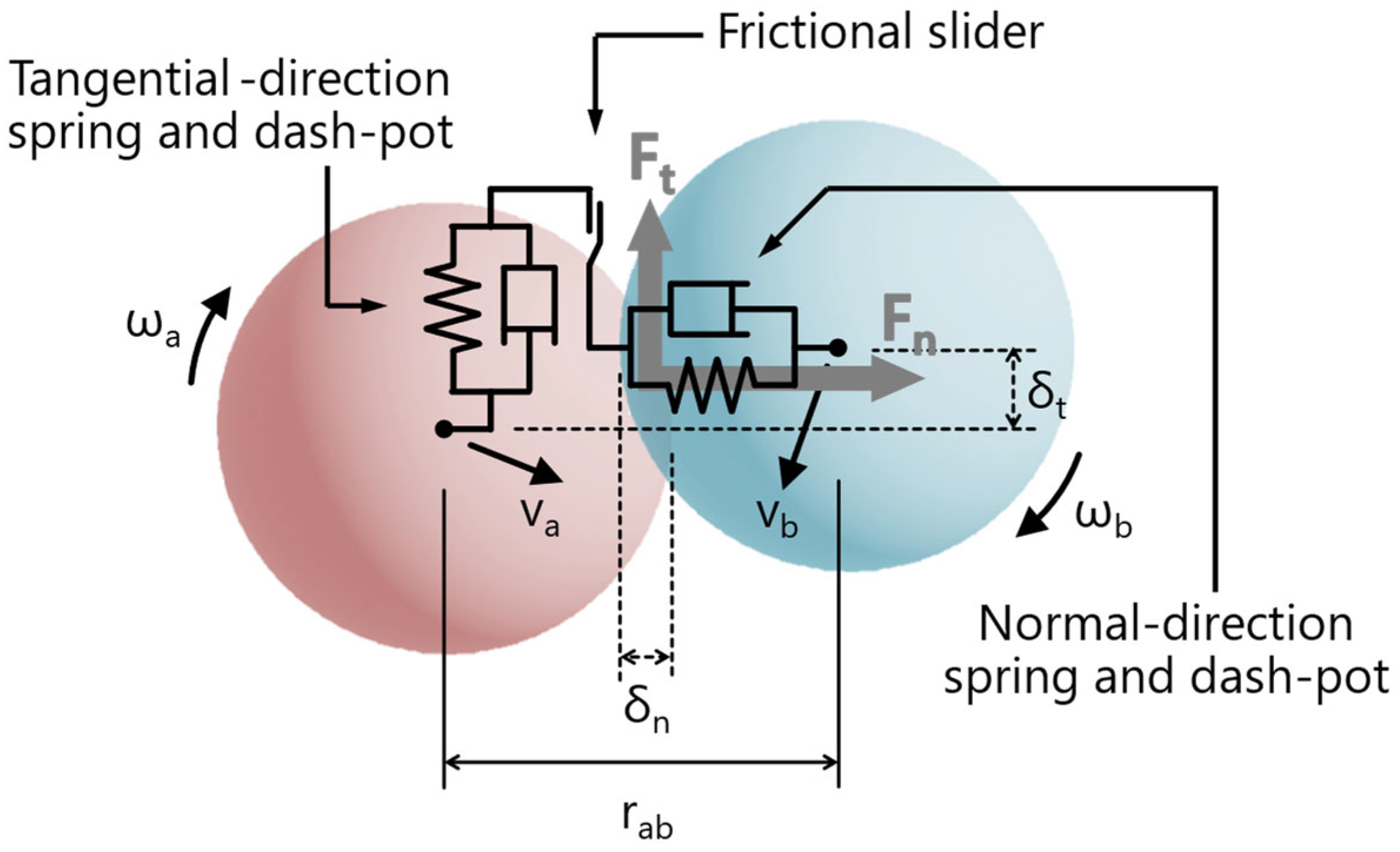
The simulation will model the pore structure of the ground and waste landfill sites. The simulation will apply Hooke’s law and Newton’s viscous law as the most basic models. The calculation of adhesion will be ignored. The external forces in the normal direction of the contact surface, the external forces in the contact surface direction, and the moments generated due to rotation are given by the following equations [20,21,22].

$${\mathit{F}}_{\mathit{n},ij}={\displaystyle \frac{4}{3}}{E}_{ij}{\delta }_{n,ij}^{{\displaystyle \frac{3}{2}}}\sqrt{R_{ij}}-\sqrt{{\displaystyle \frac{20}{3}}}·{\displaystyle \frac{\ln e}{\sqrt{{\left(\ln e\right)}^2+{\pi }^2}}}{\left(m_{ij}{E}_{ij}\sqrt{R_{ij}{\delta }_{n,ij}}\right)}^{1/2}{v}_{n,ij}$$

(3)

$${\mathit{F}}_{\mathit{t},ij}=-8G_{ij}{\delta }_{t,ij}\sqrt{R_{ij}{\delta }_{n,ij}}-\sqrt{{\displaystyle \frac{80}{3}}}·{\displaystyle \frac{\ln e}{\sqrt{{\left(\ln e\right)}^2+{\pi }^2}}}{\left(m_{ij}{E}_{ij}\sqrt{R_{ij}{\delta }_{n,ij}}\right)}^{{\displaystyle \frac{1}{2}}}{v}_{t,ij}\le {\mu }_{s,ij}{\mathit{F}}_{\mathit{n},ij}$$

(4)

$${\mathit{M}}_{ij}=r_{i }{\mathit{n}}_{ij}\times {\mathit{F}}_{\mathit{t},ij}-{\mu }_r{r}_i\left|{\mathit{F}}_{\mathit{n},ij}\right|{\displaystyle \frac{{\mathsf{\omega }}_{\mathit{r},ij}}{\left|{\mathsf{\omega }}_{\mathit{r},ij}\right|}}$$

(5)

where $r_{i }$is the radius of the element $i$ (m), $e$is the coefficient of restitution, ${\mu }_{s,ij}$is the coefficient of static friction, ${\mu }_r$is the coefficient of rotational friction, ${\mathit{n}}_{ij }$ is the unit vector in the direction of the normal at the contact surface with the elements $i$ and $j$, ${\mathsf{\omega }}_{\mathit{r},ij}$ is the relative angular velocity of elements $i$ and $j$ (rad/s), ${\delta }_{n,ij}$and ${\delta }_{t,ij}$are the amount of overlap (m) of the elements due to contact between elements $i$ and $j$ in the direction of the normal or tangential to the contact surface, $v_{n,ij}$and $v_{t,ij}$are the normal or tangential component of the relative velocity of elements $i$ and $j$ (m/s).

The first term on the right-hand side of Equations (3) and (4) represents the force due to Hooke’s law, which is proportional to displacement, and the second term represents Newton’s viscous force, which is proportional to velocity. The first term on the right-hand side of Equation (5) represents the moment acting on the contact surface between the particles, and the second term represents the effect of friction, which is proportional to angular velocity. $E_{ij}$ is the Young’s modulus used to calculate the contact force between elements $i$ and $j$ (Pa), $G_{ij}$ is the shear modulus used to calculate the contact force between elements $i$ and $j$ (Pa), $m_{ij}$ is the mass used to calculate the contact force between elements $i$ and $j$ (kg), $R_{ij}$ is the element radius (m) used when calculating the contact force between elements $i$ and $j$, and they are given by the harmonic mean of the quantities possessed by each element. The input parameters to the calculation are the following five: Young’s modulus, shear modulus, coefficient of restitution, coefficient of static friction, and coefficient of rotational friction. Soil particles include sand and clay, while waste includes plastic, metal, incineration ash, and several other types. By giving material constants to each type, it is possible to simulate the specific behavior of each material.

3.1.2. DEM Calculation Conditions

In this study, the following material properties were used: Young’s modulus of 355 MPa, shear modulus of 120 MPa (equivalent to a Poisson’s ratio of 0.48), material density of 2650 kg/m³, and restitution coefficient of 0.2. These values reflect the general physical properties of soil. DEM was applied in order to simulate the geometric positions of the void space of porous media created with certain conditions having different particle sizes and shapes. Since the purpose is only to create a pore structure, the effects of friction were not considered. Namely, the static friction coefficient and the rotational friction coefficient were set to zero.

The purpose of this study is to relate porous structures to the flow paths within them. DEM is used as a means to simulate porous structures. Since it is not necessary to create a strictly porous structure for this purpose, classical mechanical models, general model parameters, and zero friction are used to reduce the computational effort. The most influential factor is the particle size distribution and particle shape, which is parametrically changed in the DEM simulation for preparing the virtual ground.

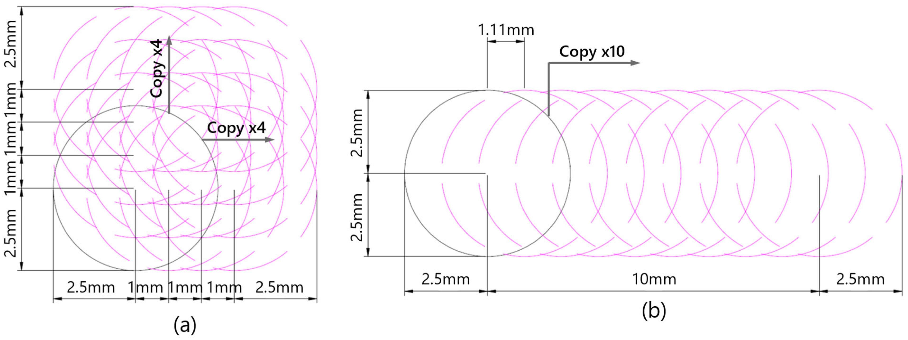
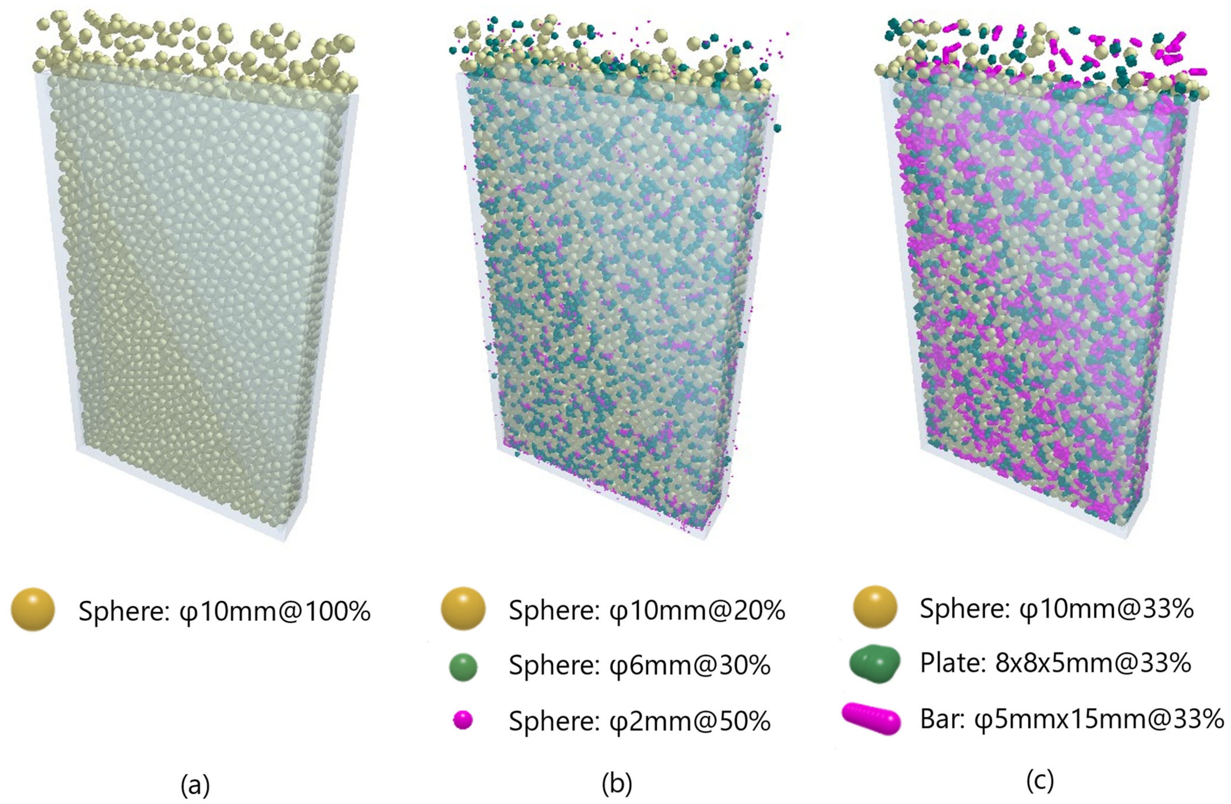
The dimensions of the analysis space were 240 mm wide, 410 mm high, and 50 mm deep, and a filling simulation was conducted by three types of freefalling samples, which have different particle sizes and shapes, from the top of the analysis space. In Case 1, only spherical elements with a uniform diameter of 10 mm were used. In Case 2, in order to simulate the ground, the particle size distribution was considered. Spherical elements with diameters of 10 mm, 6 mm, and 2 mm were mixed in a volume ratio of 2:3:5. In Case 3, assuming a waste landfill site, spherical elements with a diameter of 10 mm were mixed with thin plate elements with a width of 8 mm, depth of 8 mm, and thickness of 5 mm, and bar elements with a diameter of 5 mm and length of 15 mm in a volume ratio of 1:1:1. The thin plate element and the bar element were modeled with 5 mm diameter rigid particles at fixed intervals. The thin plate consists of 16 spherical particles arranged in a grid pattern with a particle pitch of 1 mm, and the rod-shaped particle consists of 10 spherical particles arranged in a single row. The particle pitch is 1.11 mm (see Figure 2). The calculation algorithm of DEM was referred from the OpenFOAM code documentation.

3.2. Extraction of Pore Structure from Virtual Ground

After performing DEM-based granular material filling simulations, the resulting virtual ground was visualized, and the pore structure was extracted for subsequent FEM fluid analysis. As one of the analysis results, DEM outputs the position coordinates and radius of each element filled in the analysis space as text data. By loading these text data into various viewers, it is possible to visualize the state of the analysis space after the filling simulation.

In fluid analysis aimed at evaluating the dynamics of water channels, it is necessary to extract the pore structure that exists in the gaps between each element based on the information obtained after the filling simulation. For any position ($x$, $y$, $z$) in the analysis space, it can be determined whether these are located within the element (solid) or outside the element (pore) using the following inequality.

$$\sqrt{{\left(x-x_i\right)}^2+{\left(y-y_i\right)}^2+{\left(z-z_i\right)}^2}\le r_i$$

(6)

where $x_i$ is the $x$-coordinate (m) of the center of the spherical element, $y_i$ is the $y$-coordinate (m) of the center of the spherical element and $z_i$ is the $z$-coordinate (m) of the center of the spherical element. When Equation (6) is satisfied, the corresponding position is considered to be inside the spherical element. In order to implement this discrimination process, the analysis space was divided into a grid, and discrimination using Equation (6) was carried out for each grid point ($x$, $y$, $z$). This process was applied to all spherical elements and all grid points.

However, to perform the discrimination in Equation (6) for all combinations requires a considerable amount of calculation time. Therefore, the following three approaches were used to improve the efficiency of the calculation. First, by using single-precision variables, the calculation time can be reduced compared to when double-precision variables are used. Second, when it is obvious that the inside and outside of a specific area in the analysis space can be discriminated, the processing for that area is skipped. This is due to the introduction of sub-grid technology. Thirdly, we further reduced calculation time by introducing parallel processing, taking advantage of the property that the judgment result using Equation (6) does not affect subsequent judgments. The visualization of the virtual ground and extraction of the pore structure shown in this section were carried out using the technical computing language environment MATLAB R2024a (The MathWorks).

3.3. Pore Flow Simulation Using FEM

3.3.1. FEM Governing Equation

Fluid analysis was carried out using the pore structure extracted from the virtual ground as the analysis space. The fluid analysis in this study was conducted under the simplest conditions, i.e., assuming that the pore structure was saturated, and the following steady-state Navier–Stokes equation was used as the governing equation.

$$\rho \nabla ·\mathit{u}=0$$

(7)

$$\rho \left(\mathit{u}·\nabla \right) \mathit{u}=\nabla ·\left[-p\mathit{I}+\mu \left(\nabla \mathit{u}+{\left(\nabla \mathit{u}\right)}^{\mathrm{T}}\right)\right]+\rho \mathit{g}$$

(8)

where $\rho$ is the fluid density (kg/m³), $\mathit{u}$ is the velocity vector (m/s), $p$ is the water pressure (Pa), $\mu$ is the viscosity coefficient (Pa·s), $\mathit{I}$ is the identity matrix, and $\mathit{g}$ is the gravitational acceleration vector (m/s²).

3.3.2. FEM Calculation Conditions

The parameters used in the fluid analysis were as follows: the fluid was assumed to be water, the fluid density was 1000 kg/m³, and the viscosity coefficient was 0.001 Pa·s.

The boundary conditions were set as follows: the upper surface of the analysis space was set as a rainwater infiltration boundary, with rainfall of 600 mm/yr, which is equivalent to about 1/3 of the annual rainfall in Japan. In addition, the lower surface of the analysis space was set as a pressure-fixed boundary, with a water depth of 500 mm and a water pressure of 4900 Pa. Furthermore, the no-slip condition was applied to all inner surfaces of the porous structure, and it was assumed that no flow velocity would be generated due to friction on the wall. For the initial conditions, the flow velocity vector was set to 600 mm/yr in the flow direction, and the hydrostatic pressure was set as equivalent to a water depth of 500 mm. Under these conditions, a steady-state solution was obtained. COMSOL Multiphysics ver. 6.0 (COMSOL AB), which is a numerical analysis commercial software, was used for solving the governing equations.

4. Results

4.1. Results of Virtual Ground Creation

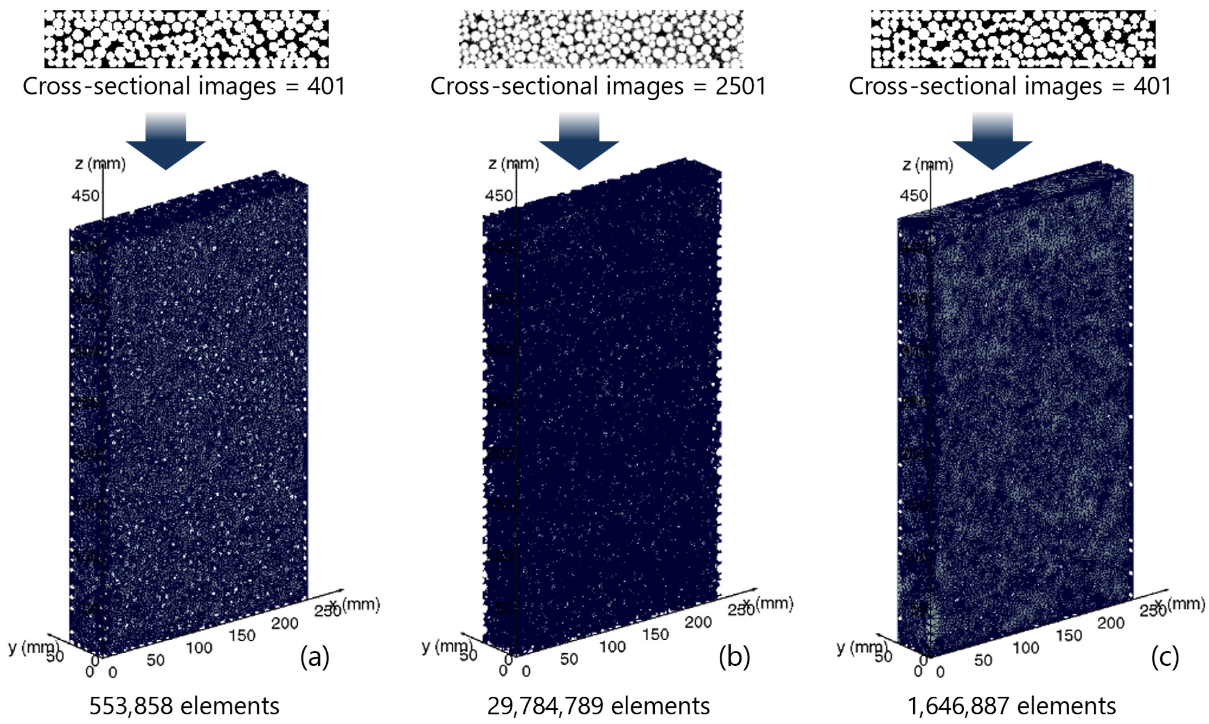
Figure 3 shows the virtual ground in which samples with different particle sizes and shapes were filled by freefall. Figure 4 is a mesh diagram of an analysis space. This is a result of judging the inside and outside of the selected position ($x$, $y$, $z$) in Equation (6), identifying the pore structure and creating a mesh that can be applied to fluid analysis. For a wider distribution and finer particle size, more detailed area determination is necessary when extracting the pore structure. As a result, the number of cross-sectional images must be increased. The three-dimensional pore structure, which is constructed by overlaying these images, significantly increases the number of elements when the mesh is processed. In Case 1, which has a uniform particle size, the pore structure could be divided into approximately 550,000 elements. In Case 2, which has a wide range of particle sizes, it was necessary to adjust the mesh width to accommodate the smaller particles, and the number of elements increased to approximately 29.78 million elements.

Fluid analysis was performed by applying the Navier–Stokes equations to the analysis space containing the constructed mesh. As Navier–Stokes equations include four unknowns, the system of linear equations became huge scale. The scale of the linear system is determined by the product of the total number of nodes and the number of unknowns. For this reason, the scale of the linear system is large in Case 2, over approximately 100 million. Specifically, the scale of the linear system in Case 1 was 8,861,728, in Case 2 was 137,821,040, and in Case 3 was 6,805,632.

A large number of cross-sectional images and a fine mesh are required to precisely extract the pore structure from a virtual ground, which contains a range of particle sizes and distributions, like the example of Case 2. As a result, the scale of the linear system to be solved increases significantly. Therefore, from the point of computational load, the effectiveness of this method is remarkable: when the range of particle size distributions is narrow, or presence of relatively fine particles does not affect global water flow, this feature is particularly useful for the analysis of waste landfill sites and gravel drainage layers. However, the size of analysis space used in this study is insufficient for a detailed analysis of water flow dynamics in waste landfill sites and gravel drainage layers. Considering the impact of scale effects on water flow, it is necessary to revise the evaluation to a larger scale. When the particle size distribution is limited and the effects of fine particles can be ignored, analysis of the flow in the pore structure with this method is considered to be advantageous in terms of reducing effort and cost.

4.2. Analysis Results of Flow in Pore Structure

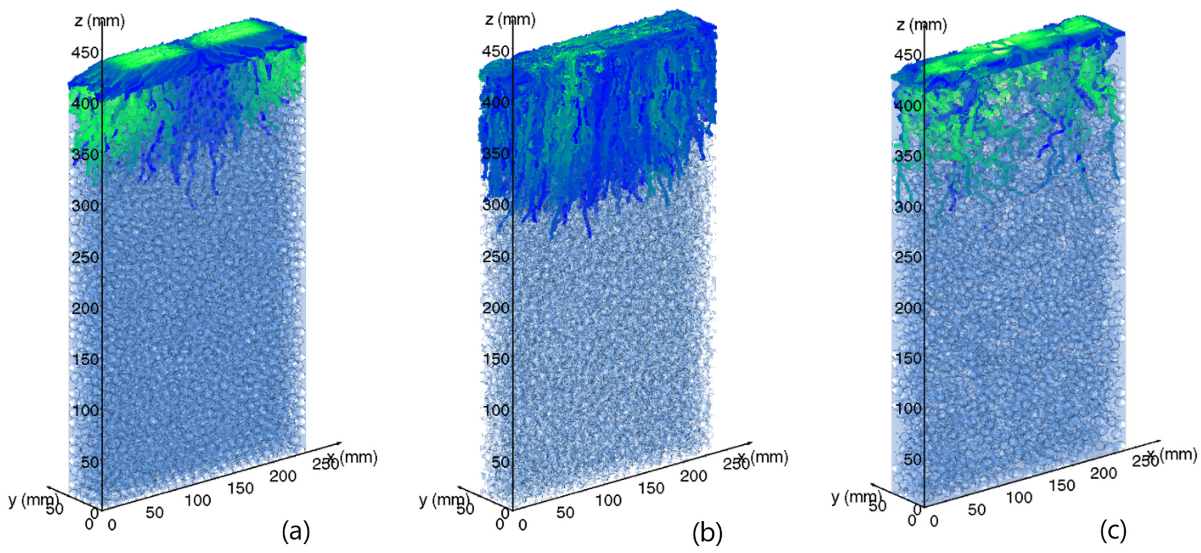
Figure 5 is the result of the fluid analysis. The streamlines are the rainwater flow path within the pore structure when a rainfall of 600 mm/yr is applied from the top surface of the analysis space.

The streamlines are obtained from the velocity vector distribution in the pore structure obtained from fluid analysis. Ten thousand tracers were uniformly placed on the top surface of the analysis space, and this was used as the starting point. The position of the tracer after a small time had elapsed was calculated by multiplying the flow velocity vector by the time step. By repeating this calculation sequentially, the trajectory of the tracer was made into a streamline. The contrast of the flow lines is the amount of tracer present along the flow path. Blue flow lines indicate that fewer tracers passed through that path, while green flow lines indicate that more tracer passed through that.

The results show that in Case 1 and Case 2, which simulate the general physical properties of soil, the streamlines extend straight in the depth direction, regardless of the starting point, indicating uniform infiltration. However, in Case 3, when thin plate and bar-shaped elements are mixed in addition to spherical elements, the streamlines are selective for certain paths of the pore structure, suggesting a water channel occurs. Therefore, it was suggested that the coupled analysis of DEM and FEM is a method capable of simulating water channels.

4.3. Tortuosity Relating to Water Channel Flow

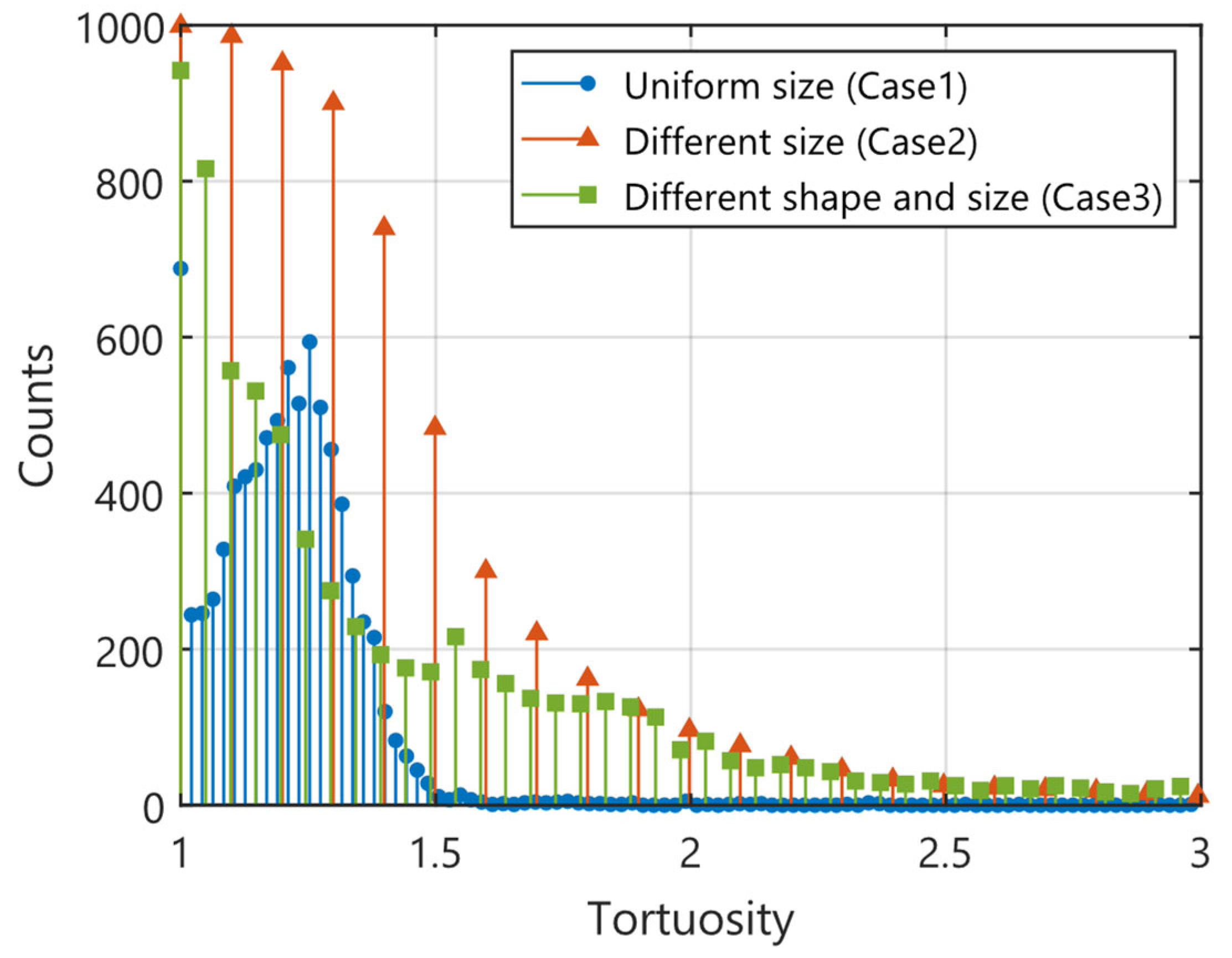
Figure 6 shows a histogram of tortuosity. Tortuosity is one of the parameters to characterize mass transport in porous media. Although mass transport is not discussed in this study, the evaluation method and results are described as a useful parameter for explaining this numerical experiment.

Tortuosity is the ratio of flow paths traveled by the tracer to the straight-line distance. Two arbitrary points in a porous medium are selected as the start and end points. The distance traveled by the tracer can be calculated using the streamlines described above. The straight-line distance can be calculated by projecting the flow lines onto the line connecting the start and end points. This makes it possible to determine the tortuosity.

The results show that the most frequent value of tortuosity in the virtual ground with uniform spherical size (Case 1) was 1.258. In Cases 2 and 3, the most frequent value was closer to 1, although the shape of a histogram was more widely spread than Case 1. In Case 2, despite the heterogeneity of particle size, the flow remained mainly uniform. The median value in Case 2 was 1.218, which was almost the same as that in Case 1.

In contrast, Case 3 (containing thin plate and rod-shaped particles) exhibited a broader and more skewed distribution, with a noticeable increase in the number of tracers following low-tortuosity paths (e.g., median values near 1.051). This suggests that water flow was selectively channeled through preferential pathways, while other regions exhibited minimal flow. The shift in tortuosity toward lower values, accompanied by increased variance, provides quantitative evidence of water channel formation.

Therefore, tortuosity analysis complements streamline visualization and provides a statistical means to detect and compare the presence and extent of water channel flow across different porous structures. This highlights the potential of the proposed framework, not only for qualitative reproduction but also for the quantitative characterization of water channels in heterogeneous landfill-like media. The calculation of the tortuosity based on the streamlines shown here is conducted only in the flow direction. As a note of caution, the obtained tortuosity is thought to be a parameter close to the longitudinal dispersion length, not a parameter that is multiplied by the molecular diffusion coefficient.

4.4. Computational Load of Numerical Experimental Method

The evaluation of the practicality of the numerical experimental method is shown in

Table 1. Computational resources required for each case study in DEM-FEM simulations, including CPU time, memory usage, and mesh resolution. Case 2, with a wide range of particle sizes, resulted in the highest computational demand due to increased mesh complexity.

		DEM Filling Simulation		FEM Fluid Simulation
		CPU Time	Image Processing Time	Mesh Count	Required Memory	CPU Time
Case 1	Uniform particles	0.5 h	5 min	553,858	30 GB	3 min
Case 2	Particle size distribution	6 h	18 h	29,784,789	312 GB	1 h 58 min
Case 3	Mixed plates and bars	3 h	6 min	1,646,887	24 GB	4 min

. The computer used in this study was equipped with a Xeon Gold 6240R (2.40 GHz, 48 cores) CPU and 384 GB of memory. A large amount of memory was required for Case 2, which took into account the particle size distribution. As for Cases 1 and 3, on the other hand, the experiments were performed within a relatively realistic calculation time. The latest advances in computer performance and the software that supports them have made it possible to evaluate the flow of large fields, which had been experimentally impossible for the time and cost involved. This method is expected to be applied to reviewing waste landfill sites and gravel drainage layers as a countermeasure against recent extreme weather conditions and even to strengthen the final disposal sites.

5. Discussion

The novelty of this study lies in its integrated simulation framework, which, for the first time, incorporates non-spherical particles, such as thin plates and rods, into a coupled DEM-FEM model for simulating water flow in heterogeneous porous media. This approach addresses a significant gap in previous research, where most DEM-based simulations have been limited to spherical or simplified particle geometries. By considering more realistic particle shapes, the proposed model more accurately reproduces the variability in pore structure and the resulting water channel flow behavior often observed in landfill layers.

Another important contribution of this framework is its ability to overcome the limitations of conventional experimental methods such as X-ray computed tomography (CT). In the analysis of landfill waste, X-ray CT has limitations, such as a penetration depth of only a few centimeters, sensitivity to noise from metals, and the inability to study heterogeneities at actual scales. In contrast, the numerical approach in this study enables the large-scale three-dimensional reconstruction of pore structure and fluid flow fields using adjustable parameters and controlled geometric shapes.

Despite its strengths, several limitations need to be addressed in future work to improve the applicability and reliability of this method. First, the current framework is proposed as a proof of concept and has not yet reached the stage of providing statistically representative results. To make quantitative conclusions, multiple simulations under specific conditions will be required to evaluate the variability in the flow paths and extract meaningful averages.

Second, the virtual porous media in this study were generated by freefalling deposition with simplified and fixed DEM parameters. Frictional effects were intentionally neglected to reduce the computational effort. However, in real landfills, compaction processes, particle deformability, and non-uniform loading conditions significantly affect pore connectivity. Therefore, further development should include sensitivity analyses for DEM parameters and the implementation of more realistic boundary conditions and scaling considerations.

In addition, experimental validation of the simulated flow structures is a major challenge. Real-time, three-dimensional visualization of water channel flow remains technically challenging. Techniques such as time-lapse electrical resistivity tomography (ERT) [23] or particle image velocimetry (PIV) [24] can provide validation but are often expensive and require specialized instrumentation. Thus, the development of simplified yet effective methods for validating water channels in porous media remains an open research frontier.

In conclusion, while the proposed DEM-FEM framework represents a significant step forward in modeling complex flow pathways in heterogeneous waste media, further refinement and validation are necessary to establish its practical utility and robustness for engineering and environmental applications.

6. Conclusions

This study proposes a computer-based numerical experimental method that combines the discrete element method (DEM) and the finite element method (FEM). The purpose is to replace research on waste landfill layers and gravel drainage layers, which tend to be large-scale experiments.

In this study, the performance of this method was evaluated targeting the flow in porous media. This method is effective for flow analysis when the particle size distribution of the sample is limited, and the fine particle size does not have a large effect on the global water channels. Its specific examples include waste landfill layers and crushed stone drainage layers.

However, many points for improvement were identified. Simulations need to be modified to take into account the effects of external forces caused by compaction, which occurs in real landfill operations, rather than freefall. We need to reconsider how soft materials deform and how landfill waste becomes compacted. In addition, the phenomenon in which the initial air present in the pore is trapped within it by rainwater infiltration should also be investigated. These phenomena could be related to the infiltration behavior in the virtual ground and be a formation factor of water channels, suggesting computational methods to simulate this phenomenon are necessary. An approach based on the local reality is considered to be an important technical element in revealing accurate water channels.

In further research, the goal is to refine the analytical methods to clarify the dynamics of water channels, while at the same time developing experimental techniques to verify the water channels obtained using this numerical experimental method.

References

- Glass, R.J.; Nicholl, M.J. Physics of gravity fingering of immiscible fluids within porous media: An overview of current understanding and selected complicating factors. Geoderma 1996, 70, 133–163. [Google Scholar] [CrossRef]
- Onody, R.N.; Posadas, A.N.D.; Crestana, S. Experimental studies of the fingering phenomena in two dimensions and simulation using a modified invasion percolation model. J. Appl. Phys. 1995, 78, 2970–2976. [Google Scholar] [CrossRef]
- Wang, Z.; Wu, L.S.; Harter, T.; Lu, J.H.; Jury, W.A. A field study of unstable preferential flow during soil water redistribution. Water Resour. Res. 2003, 39, 1075. [Google Scholar] [CrossRef]
- Ishimori, H.; Isobe, Y.; Ishigaki, T.; Yamada, M. Undisturbed sampling of waste layer and its x-ray CT image analysis for estimating water channel flow. In Proceedings of the 11th Asia-Pasific Landfill Symposium, Bangkok, Thailand, 8–10 November 2022; pp. 191–196. [Google Scholar]
- Zeng, Q.Y.; Zheng, M.X.; Huang, D. Numerical simulation of impact and entrainment behaviors of debris flow by using SPH-DEM-FEM coupling method. Open Geosci. 2022, 14, 1020–1047. [Google Scholar]
- Chen, H.S.; Liu, W.W.; Li, S.Q. A fully-resolved LBM-LES-DEM numerical scheme for adhesive and cohesive particle-laden turbulent flows in three dimensions. Powder Technol. 2024, 440, 119800. [Google Scholar] [CrossRef]
- Li, L.; Xu, P.; Li, Q.; Zheng, R.; Xu, X.; Wu, J.; He, B.; Bao, J.; Tan, D. A coupled LBM-LES-DEM particle flow modeling for microfluidic chip and ultrasonic-based particle aggregation control method. Appl. Math. Model. 2025, 143, 116025. [Google Scholar] [CrossRef]
- Cao, R.Y.; Li, Y.P.; Feng, C.; Fan, L.; Liu, W.Y.; Zhang, Y.M. Study on the Damage Effects of Explosive Media Based on FEM-DEM Local Adaptive Transformation. Geotech. Geol. Eng. 2024, 42, 339–350. [Google Scholar] [CrossRef]
- Li, X.K.; Wang, Z.; Du, Y.; Duan, Q. Advances in Multiscale FEM-DEM Modeling of Granular Materials. In Proceedings of the 7th International Conference on Discrete Element Methods, Dalian, China, 1–4 August 2016; pp. 267–279. [Google Scholar]
- Nilsen, H.M.; Larsen, I.; Raynaud, X. Combining the modified discrete element method with the virtual element method for fracturing of porous media. Comput. Geosci. 2017, 21, 1059–1073. [Google Scholar] [CrossRef]
- Pirnia, P.; Duhaime, F.; Ethier, Y.; Dubé, J.S. ICY: An interface between COMSOL multiphysics and discrete element code YADE for the modelling of porous media. Comput. Geosci. 2019, 123, 38–46. [Google Scholar] [CrossRef]
- Wang, K.; Sun, W.C. A semi-implicit discrete-continuum coupling method for porous media based on the effective stress principle at finite strain. Comput. Methods Appl. Mech. Eng. 2016, 304, 546–583. [Google Scholar] [CrossRef]
- Wang, K.; Sun, W.C. A multiscale multi-permeability poroplasticity model linked by recursive homogenizations and deep learning. Comput. Methods Appl. Mech. Eng. 2018, 334, 337–380. [Google Scholar] [CrossRef]
- Wang, K.; Sun, W.C. An updated Lagrangian LBM-DEM-FEM coupling model for dual-permeability fissured porous media with embedded discontinuities. Comput. Methods Appl. Mech. Eng. 2019, 344, 276–305. [Google Scholar] [CrossRef]
- Liu, G.R.; Liu, M.B. Smoothed Particle Hydrodynamics a Meshfree Particle Method; World Scientific Publishing Co. Pte. Ltd.: Singapore, 2003. [Google Scholar]
- Sigalotti, L.D.; Klapp, J.; Gesteira, M.G. The Mathematics of Smoothed Particle Hydrodynamics (SPH) Consistency. Front. Appl. Math. Stat. 2021, 7, 797455. [Google Scholar] [CrossRef]
- Lind, S.J.; Rogers, B.D.; Stansby, P.K. Review of smooth particle hydrodynamics: Towards converged Lagrangian flow modelling. Proc. R. Soc. A Math. Phys. Eng. Sci. 2020, 476, 20190801. [Google Scholar] [CrossRef]
- Yazdchi, K.; Srivastava, S.; Luding, S. FEM-DEM Simulation of Two-way Fluid-Solid Interaction in Fibrous Porous Media. In Proceedings of the 7th International Conference on Micromechanics of Granular Media (Powders and Grains), Sydney, Australia, 8–12 July 2013; Volume 1542, pp. 1015–1018. [Google Scholar]
- Xu, W.X.; Zhang, B.; Jia, M.K.; Wang, W.; Gong, Z.; Jiang, J.Y. Discrete element modeling of 3D irregular concave particles: Transport properties of particle-reinforced composites considering particles and soft interphase effects. Comput. Methods Appl. Mech. Eng. 2022, 394, 114932. [Google Scholar] [CrossRef]
- Hund, D.; Weis, D.; Hesse, R.; Antonyuk, S. Simulation study of the discharge characteristics of silos with cohesive particles. In Proceedings of the 8th International Conference on Micromechanics on Granular Media, Montpellier, France, 3–7 July 2017; p. 08015. [Google Scholar] [CrossRef]
- Ramírez-Aragón, C.; Ordieres-Mere, J.; Alba-Elías, F.; González-Marcos, A. Comparison of Cohesive Models in EDEM and LIGGGHTS for Simulating Powder Compaction. Materials 2018, 11, 2341. [Google Scholar] [CrossRef] [PubMed]
- Wilkinson, S.K.; Turnbull, S.A.; Yan, Z.; Stitt, E.H.; Marigo, M. A parametric evaluation of powder flowability using a Freeman rheometer through statistical and sensitivity analysis: A discrete element method (DEM) study. Comput. Chem. Eng. 2017, 97, 161–174. [Google Scholar] [CrossRef]
- Sejati, P.A.; Saito, N.; Prayitno, Y.A.K.; Tanaka, K.; Darma, P.N.; Arisato, M.; Nakashima, K.; Takei, M. On-line multi-frequency electrical resistance tomography (MFERT) device for crystalline phase imaging in high-temperature molten oxide. Sensors 2022, 22, 1025. [Google Scholar] [CrossRef] [PubMed]
- Arthur, J.K. PIV and refractive index matching in porous media. Adv. Water Resour. 2020, 146, 103793. [Google Scholar] [CrossRef]
Figure 1.
Diagram explaining the forces and parameters acting between two particles. The normal force (Fn) and the tangential force (Ft) acting between particles are given by the sum of Hooke’s law, which is proportional to displacement (δ), and Newton’s law of viscosity, which is proportional to velocity (v).
Figure 2.
Modeling of non-spherical particles using rigidly connected spherical elements. (a) Thin plate model composed of 16 spherical elements (diameter: 5 mm) arranged in a 4 × 4 grid with a center-to-center spacing of 1 mm; (b) rod-shaped model composed of 10 spherical elements (diameter: 5 mm) aligned in a straight line with a spacing of 1.11 mm.
Figure 3.
Virtual ground models generated via DEM-based freefall simulations for three cases: (a) uniform spherical particles (Case 1); (b) mixed spherical particles with different diameters (Case 2); and (c) mixed spherical, thin plate, and rod-shaped particles (Case 3). These configurations represent idealized ground, particle-size-distributed ground, and heterogeneous waste-like landfill, respectively.
Figure 4.
Finite element meshes generated from extracted pore structures of each virtual ground case: (a) uniform spherical particles (Case 1); (b) mixed spherical particles with different diameters (Case 2); and (c) mixed spherical, thin plate, and rod-shaped particles (Case 3). These meshes were used for fluid analysis and vary in resolution due to differences in particle configuration and size distribution.
Figure 5.
Streamlines indicating simulated rainwater infiltration paths in the pore structure, derived from DEM-FEM coupled analysis under steady-state conditions: (a) uniform spherical particles (Case 1); (b) mixed spherical particles with different diameters (Case 2); and (c) mixed spherical, thin plate, and rod-shaped particles (Case 3). Preferential flow paths are observed in Case 3 due to the inclusion of non-spherical particles, suggesting the formation of water channels.
Figure 6.
Histogram of tortuosity values calculated from each streamline trajectory. Tortuosity represents the ratio of the actual tracer path length to the straight-line distance and reflects the complexity of the pore geometry. A broader distribution in Case 3 indicates more irregular flow paths due to structural heterogeneity.