Real-Time Sea State Estimation for Wave Energy Converter Control via Machine Learning

Abstract

Wave energy converters (WECs) harness the untapped power of ocean waves to generate renewable energy, offering a promising solution to sustainable energy. An optimal WEC control strategy is essential to maximize power capture that dynamically adjusts system parameters in response to rapidly changing sea states. This study presents a novel control approach that leverages neural networks to estimate sea states from onboard WEC measurements such as position, velocity, and force. Using a point absorber WEC device as a test platform, our proposed approach estimates sea states in real-time and subsequently adjusts PID controller gains to maximize energy extraction. Simulation results across diverse sea conditions demonstrate that our strategy eliminates the need for external wave monitoring equipment while maintaining power capture efficiency. The results show that our neural network-based control technique can improve power capture by 25.6% while significantly reducing system complexity. This approach offers a practical alternative for WEC deployments where direct wave measurements are either infeasible or cost prohibitive.

1. Introduction

Harnessing ocean wave energy offers a promising renewable energy resource by exploiting the vast and consistent energy of the ocean. Wave energy converters (WECs) face significant challenges in achieving efficient energy conversion due to the dynamic and unpredictable nature of ocean waves [1]. Effective control strategies are crucial to ensure that WECs operate optimally and safely under these varying conditions, although developing such strategies is a challenging task.

Several types of WEC control strategies have been widely explored in the literature. These strategies mainly utilize predefined incoming ocean wave characteristics to optimize control actions and maximize energy extraction. Model predictive control (MPC) is a popular approach for WECs when wave profiles are known, and it can be used in diverse sea state conditions while obeying system constraints. Fusco and Ringwood [2] introduced an MPC framework that used wave profile information to optimize Power Take-Off (PTO) forces for enhanced energy absorption. Similarly, Henriques et al. [3] demonstrated simplified wave models for MPC, improving real-time performance. Complex conjugate control (CCC) maximizes power transfer by matching the impedance of the WEC to the incoming wave. Foundational work by Falnes [4] showed that known wave excitation forces allow impedance matching for optimal energy transfer. However, CCC is non-causal, as it requires future knowledge of wave forces. Li and Belmont [5] developed predictive approximations to make CCC viable in real-time applications. Feedback resonating control (FBR) tested by Coe et al. [6] shows promising results by leveraging known sea states to adjust resonance frequencies. Proportional–integral–derivative (PID) controllers, often adapted with wave prediction, have also been studied in the WEC context. Yu and Falnes [7] demonstrated that PID control tuned to anticipated wave periods and amplitudes allowed WECs to track wave oscillations effectively. Adaptive PID gains, as seen in the work of Vantorre et al. [8], further improved performance over short intervals as wave conditions varied. In parallel, classical state-estimation algorithms such as Kalman filtering [9], the Extended Kalman Filter (EKF) [10], and the Unscented Kalman Filter (UKF) [11] have long been used to infer unmeasured dynamic states under linear or mildly nonlinear models and Gaussian noise assumptions. Particle filters [12] generalize this to highly nonlinear, non-Gaussian settings via sequential Monte Carlo sampling. In the WEC domain, Coe et al. [6] demonstrated a Kalman-based wave-prediction scheme to infer excitation forces from onboard measurements, though its accuracy degrades under model mismatch and non-Gaussian disturbances. Linear quadratic regulator (LQR) controllers [13] optimize a quadratic cost around a fixed linearization, requiring re-linearization or gain scheduling as sea conditions change. A central assumption for these approaches is to have a well-defined model representation of the WEC device, which is often computationally expensive given diverse sea conditions.

Machine learning techniques, particularly deep learning, have recently emerged as promising tools for WEC control due to their adaptability and ability to generalize across diverse conditions [14,15]. In wave energy research, deep neural networks (DNNs) have been explored for predicting wave characteristics based on historical data and WEC operational parameters [16]. These studies suggest that DNNs can be effective in identifying patterns in highly variable data, enabling WECs to respond more flexibly to changing ocean states without direct wave measurements. More recently, reinforcement learning has been applied to optimize control based on known sea states. Duarte and Sarmento [17] developed a reinforcement learning-based controller trained on wave data, predicting control actions across various sea states. These methods show promise but require extensive training data and computational resources, limiting practical WEC deployment in real ocean environments. Despite control approaches from different angles, estimating incoming wave or sea state from the physical measurements of the WEC device remains limited.

Despite these advancements, most WEC control strategies rely on direct wave measurements using buoys, radar, or pressure sensors to optimize power capture. But these approaches are costly, maintenance intensive, and vulnerable to harsh marine conditions. Real-time data acquisition also introduces latency and communication constraints, limiting its effectiveness for dynamic control. Moreover, wave sensors can fail or become impractical in extreme environments, making them unreliable for long-term deployment. These challenges highlight the need for an alternative approach that eliminates dependence on external wave measurements. Machine learning, particularly deep learning, offers a potential solution by extracting meaningful patterns from these onboard measurements. Neural networks have shown success in renewable energy applications [14], including wave prediction [16], but their use in WEC control remains underexplored. Furthermore, while nonlinear model-based controllers can handle system uncertainties, they require detailed parametric models and the extensive tuning of control parameters, which may be impractical under rapidly changing sea states. Reinforcement-learning-based tuning methods such as DDPG offer end-to-end policy optimization but demand large volumes of training data and online exploration, posing safety and sample-efficiency challenges in marine environments.

To overcome these challenges, we propose a machine learning-based control strategy that estimates sea states directly from onboard WEC measurements (position, velocity, and force), eliminating the need for external wave sensors. In this study, we develop and evaluate a long short-term memory (LSTM)-based control framework that uses physical data from the WEC itself to predict the incoming wave spectrum, aiming to improve energy capture efficiency and device adaptability under real-world conditions. By training and validating the model across a broad range of operational scenarios, we demonstrate how this control strategy enhances WEC performance by making it more responsive and resilient to changing ocean waves. We propose a novel LSTM-based framework for real-time sea-state estimation using only onboard WEC measurements, and integrate this estimator into a supervisory control loop that updates PID gains every 10 s. Through comprehensive simulations, we demonstrate that this adaptive approach achieves a 25.6% increase in power capture under variable sea conditions relative to fixed-gain PI control. Furthermore, we show robustness to model mismatch by employing noise-augmented training during model development. This research contributes to advancing wave energy technology by addressing key limitations in current control strategies, potentially enabling more efficient and sustainable ocean energy solutions.

This paper is structured as follows. Section 2 describes the WaveBot dynamics. Section 3 introduces our LSTM-based estimation framework and supervisory control. Section 4 details the PI-gain design and stability analysis. Section 5 presents the simulation results under fixed and variable seas. Section 6 discusses the implications, and Section 7 concludes.

2. WEC Device

2.1. WaveBot Device Specifications

The WaveBot is a point absorber type of WEC device that operates as a heaving buoy using a PTO mechanism that translates vertical oscillations into rotational energy. This design enables effective energy extraction by directly converting wave motion into electrical power. WaveBot employs a rack-and-pinion mechanism with a high gear ratio, enhancing the rotational velocity transferred to the PTO and maximizing power generation. Essential device specifications are listed in

Table 1. WaveBot physical parameters.

Parameter	Value	Unit
Rigid body mass, m	875	kg
Hydrostatic stiffness, $k_h$	2.44	kN/m
Linear friction coefficient, $b_f$	1	Ns/m
Gear ratio, N	12.4666	rad/m
Shaft inertia, $J_d$	2	kg m²
Torque constant, $k_{\tau }$	6.1745	Nm/A
Motor winding resistance, $R_w$	0.5	$\Omega$

, which shows the WaveBot’s primary components and energy conversion stages. An illustration of the device is shown in Figure 1.

2.2. WEC Dynamics

The dynamics of a WEC operating in heave can be described by considering all forces acting on the system as shown in Equation (1):

$$m·a=F_{\mathrm{exc}}+F_{\mathrm{rad}}+F_{\mathrm{hydro}}+F_{\mathrm{fric}}-F_{\mathrm{pto}}$$

(1)

where m is the mass of the WEC, a is the vertical acceleration of the WEC, $F_{\mathrm{exc}}$ is the excitation force exerted by incoming ocean waves, $F_{\mathrm{rad}}$ is the radiation force modeling the reactive effect of water due to the movement of the WEC, $F_{\mathrm{hydro}}$ is the hydrostatic restoring force reflecting the balance of buoyancy and gravity, $F_{\mathrm{fric}}$ is the frictional force from internal damping within the WEC system, and $F_{\mathrm{pto}}$ is the PTO force, which opposes the motion of the WEC to extract energy [4].

For maximum power absorption, mechanical impedance matching is applied by aligning the PTO impedance $Z_{\mathrm{pto}}\left(\omega \right)$ with the complex conjugate of the intrinsic mechanical impedance of WEC, $Z_i\left(\omega \right)$ [18], where

$$Z_i\left(\omega \right)=B\left(\omega \right)+b_f+j\left(\omega \left(m+A\left(\omega \right)\right)-{\displaystyle \frac{k_h}{\omega }}\right)$$

(2)

The WaveBot’s dynamics are driven by a combination of wave excitation forces, PTO forces, and the system’s intrinsic mechanical impedance. The linear equation of motion for vertical displacement in response to wave-induced forces is given by   

$$F_{\mathrm{exc}}V\left(\omega \right)-F_{\mathrm{pto}}V\left(\omega \right)=Z_{i}V\left(\omega \right)·V\left(\omega \right)$$

(3)

Here, $B\left(\omega \right)$ represents the radiation damping, $A\left(\omega \right)$ denotes the added mass, and $\omega$ is the angular frequency of the oscillatory motion. This impedance is a function of the device’s hydrodynamic properties and acts as a frequency-dependent resistance to vertical motion. The optimal condition for power transfer is achieved by setting

$$F_{\mathrm{pto},\mathrm{opt}}\left(\omega \right)=Z_{\mathrm{pto}}\left(\omega \right)V\left(\omega \right)=Z_i^{*}\left(\omega \right)V\left(\omega \right)$$

(4)

This optimal control law can be approximated in sea states dominated by one frequency as a proportional–integral feedback law

$$F_{\mathrm{pto},\mathrm{opt}}\left(\omega \right)\approx Z_{\mathrm{pto},\mathrm{PI}}\left(\omega \right)V\left(\omega \right)=\left(K_P+{\displaystyle \frac{K_I}{jw}}\right)V\left(\omega \right)$$

(5)

To maximize power transfer, we approximate $Z_{\mathrm{pto},\mathrm{PI}}\left(\omega \right)$ to match $Z_i^{*}\left(\omega \right)$ within the range of frequencies where the wave excitation is significant. This approach results in the following conditions for the PI controller gains:

$$K_P=B\left(\omega \right)+b_f$$

(6)

$$K_I={\omega }^2(m+A\left(\omega \right))-k_h$$

(7)

3. Proposed Control Approach

WEC Control by Sea State

WEC control traditionally relies on anticipating and responding to incoming ocean wave to maximize energy capture. In a study by Coe et al. (2018), several WEC control methods are evaluated, including FBR control and MPC [6]. These approaches attempt to match the controller’s response to wave characteristics, often through wave prediction. However, capturing wave profiles directly requires additional equipment like auxiliary measurement buoys, leading to increased complexity, cost, and reliability issues.

In contrast to direct measurement, we propose a control strategy that predicts sea states based on the velocity, position, and PTO force of the WEC device. By analyzing these parameters, our approach identifies the sea state that would produce the observed WEC dynamics, allowing the dynamic selection of optimal control gains. This method leverages readily accessible metrics, eliminating the need for direct wave measurements. The prediction is inherently reactive to the WEC’s real-time response, reducing delay and uncertainty while achieving high energy capture with less complexity.

The proposed WEC control method begins by collecting readily measurable parameters from the WEC, specifically the device’s position (z), velocity ($\dot{z}$), and the PTO force ($F_{\mathrm{PTO}}$), which are essential indicators of the interaction of the WEC with incoming waves. These parameters are then used as inputs to a neural network model that predicts sea state characteristics, i.e., peak wave period ($T_p$).

A JONSWAP spectrum in terms of sea states can be expressed as follows:

$$S\left(\omega \right)={\displaystyle \frac{\alpha g^2}{{\omega }^5}}exp\left(-{\displaystyle \frac{5}{4}}{\left({\displaystyle \frac{\omega }{{\omega }_p}}\right)}^{-4}\right){\gamma }^{exp\left(-{\displaystyle \frac{{(\omega -{\omega }_p)}^2}{2{\sigma }^2{\omega }_p^2}}\right)}$$

(8)

where

$$\begin{array}{c}\hfill \alpha ={\displaystyle \frac{5}{16}}{\displaystyle \frac{H_m^2}{T_p^4}},{\omega }_p={\displaystyle \frac{2\pi }{T_p}},\sigma =\left\{\begin{array}{cc}0.07,\hfill & \mathrm{if}\omega \le {\omega }_p,\hfill \\ 0.09,\hfill & \mathrm{if}\omega >{\omega }_p\hfill \end{array}\right.\end{array}$$

where we have the following: $\alpha$ is the Phillips parameter, controlling the overall amplitude of the spectrum; g is gravitational acceleration; $\omega$ is the wave frequency; ${\omega }_p$ is the peak wave frequency; $\gamma$ is the peak enhancement factor; and $\sigma$ is the spectral width parameter, with typical values of $\sigma =0.07$ for $\omega <{\omega }_p$ and $\sigma =0.09$ for $\omega \ge {\omega }_p$.

The neural network model is trained and fine-tuned by incorporating additive white Gaussian noise (AWGN) to improve robustness in noisy conditions. Once the sea state parameter $T_p$ is predicted, it is mapped to obtain optimal controller gains ($K_P$ and $K_I$) for a PID controller. This enables dynamic adjustment of the control actions to match the identified sea state characteristics and maximize energy absorption. Figure 2 represents the overall proposed approach showing the input excitation force, $F_{exec}$, and primary and supervisory control blocks to obtain the desired PTO force, $F_{PTO}^{*}$. Primary control is the conventional PID control block, which takes peak periods ($T_p$) of sea states as input. The supervisory control block is the neural network approach that takes features from the WEC physical parameters and estimates the corresponding $T_p$. The WEC system was obtained for a sample time of 0.1 s, and hence the step time for both supervisory and primary control blocks is kept at 0.1 s.

4. Control Design

The primary objective of the WEC control system is to maximize power capture while maintaining stability across varying sea states. In this study, a PI controller is implemented, where the gains $K_P$ and $K_I$ are computed based on the mechanical impedance of the system rather than an optimization-based tuning approach.

The PI controller regulates the response of the WEC to ocean waves, ensuring optimal energy harvesting. The controller transfer function is given by

$$C(\omega ;K_P,K_I)=K_P-i{\displaystyle \frac{K_I}{\omega }},$$

(9)

where $K_P$ and $K_I$ represent the proportional and integral gains, respectively, and $\omega =2\pi f$ is the angular frequency.

Instead of determining $K_P$ and $K_I$ through numerical optimization, the new approach computes the gains directly from the system’s mechanical impedance. The state-space representation of the WEC device is given by

$$\mathbf{x}[k+1]=A\mathbf{x}\left[k\right]+B\mathbf{u}\left[k\right],$$

(10)

$$\mathbf{y}\left[k\right]=C\mathbf{x}\left[k\right]+D\mathbf{u}\left[k\right],$$

(11)

where $A,B,C,$ and D are the state-space matrices representing the system dynamics.

The mechanical impedance of the WEC is derived from the system’s transfer function. Given a wave period T, the corresponding frequency is $\omega ={\displaystyle \frac{2\pi }{T}}$.

Using a discrete-time representation, the transfer function $H\left(z\right)$ is computed as

$$H\left(z\right)=C{(zI-A)}^{-1}B+D,$$

(12)

where $z=e^{j\omega T_s}$ is the discrete-time frequency response variable, and $T_s$ is the sampling time:

$$K_P=\mathrm{Re}\left(Z_{\mathrm{mech}}^{*}\right),$$

(13)

$$K_I=-\omega ·\mathrm{Im}\left(Z_{\mathrm{mech}}^{*}\right).$$

(14)

To ensure stability and prevent extreme values, $K_P$ and $K_I$ are constrained within predefined limits: $K_P\in [0,5·{10}^3],K_I\in [-2·{10}^4,1·{10}^6]$. Details on the impedance-based WEC control design, and performance and stability considerations can be found in [6,18].

This method allows for the real-time adaptation of control gains based on sea state variations without requiring iterative numerical optimization, improving computational efficiency and robustness. The implementation is carried out in MATLAB, where the PI gains are computed dynamically based on the measured wave period $T_p$.

4.1. Neural Network Modeling

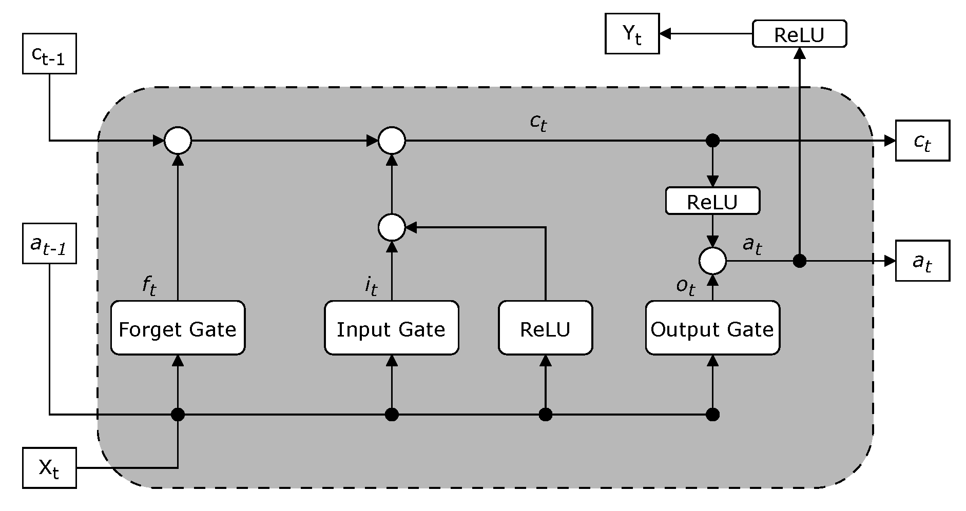
In this study, we used a deep learning model named Long Short-Term Memory (LSTM) network, which is a class of recurrent neural networks (RNNs). This model can handle sequential data by addressing the vanishing gradient problem encountered in traditional RNNs. Unlike conventional feedforward neural networks, LSTMs maintain an internal memory state, allowing them to capture long-range dependencies in time-series data. This makes them particularly well suited for problems involving temporal patterns, which is much needed in our study of incoming wave prediction.

As shown in Figure 3, an LSTM cell consists of three primary gates: the forget gate, the input gate, and the output gate, which regulate the flow of information through the network. The LSTM cell updates its cell state $C_t$ and hidden state $h_t$ at each time step t based on the previous hidden state $h_{t-1}$, the previous cell state $C_{t-1}$, and the current input $x_t$. The update process is given by the following equations:

$$\begin{array}{}\mathrm{(15)}& f_t=\sigma (W_f{x}_t+U_f{h}_{t-1}+b_f)\hfill & \hfill (\mathrm{Forget}\mathrm{Gate})\mathrm{(16)}& i_t=\sigma (W_i{x}_t+U_i{h}_{t-1}+b_i)\hfill & \hfill (\mathrm{Input}\mathrm{Gate})\mathrm{(17)}& {\tilde{C}}_t=tanh(W_c{x}_t+U_c{h}_{t-1}+b_c)\hfill & \hfill (\mathrm{Cell}\mathrm{State}\mathrm{Candidate})\mathrm{(18)}& C_t=f_t\odot C_{t-1}+i_t\odot {\tilde{C}}_t\hfill & \hfill (\mathrm{Cell}\mathrm{State}\mathrm{Update})\mathrm{(19)}& o_t=\sigma (W_o{x}_t+U_o{h}_{t-1}+b_o)\hfill & \hfill (\mathrm{Output}\mathrm{Gate})\mathrm{(20)}& h_t=o_t\odot tanh\left(C_t\right)\hfill & \hfill (\mathrm{Hidden}\mathrm{State}\mathrm{Update})\end{array}$$

Here, $\sigma (·)$ represents the sigmoid activation function, $tanh(·)$ is the hyperbolic tangent function, and ⊙ denotes element-wise multiplication. The weight matrices $W_f,W_i,W_c,W_o$ and $U_f,U_i,U_c,U_o$ along with the biases $b_f,b_i,b_c,b_o$ are learned parameters. LSTMs outperform traditional RNNs in sequence modeling due to their ability to selectively retain or forget information over long sequences. Unlike standard feedforward networks, which process inputs independently, LSTMs utilize a gating mechanism to control information flow, enabling them to learn dependencies over extended time horizons. This is crucial for applications where past inputs influence future predictions, such as ocean wave dynamics. A detailed optimization approach for the LSTM model is presented in Algorithm 1.

Figure 3. Structure of an LSTM cell, showing the forget, input, and output gates [19].

Figure 3. Structure of an LSTM cell, showing the forget, input, and output gates [19].

Algorithm 1 LSTM estimator training and optimization.

Require: Raw WEC data $\mathcal{D}={\left\{(z_t,{\dot{z}}_t,F_{\mathrm{PTO},t},T_{p,t})\right\}}_{t=1}^M$, window length L, learning rate ${\eta }_0$, max epochs $N_{\mathrm{ep}}$ Ensure: Optimized LSTM parameters ${\theta }^{*}$     Data Preparation:     Partition $\mathcal{D}$ into overlapping windows of length L: $\{X^{\left(i\right)},y^{\left(i\right)}\}$     Normalize features in $X^{\left(i\right)}$ via min–max scaling     Augment: $X^{\left(i\right)}\leftarrow X^{\left(i\right)}+\mathcal{N}(0,{\sigma }_{\mathrm{noise}}^2)$     Split into training, validation, and test sets     Model Initialization:     Initialize LSTM parameters $\theta$ and optimizer with rate ${\eta }_0$     Set best_val_loss $\leftarrow \infty$     Training Loop:     for epoch $=1$$N_{\mathrm{ep}}$ do       Shuffle training set into mini-batches       for each batch $(X_b,y_b)$ in training set do           ${\widehat{y}}_b\leftarrow \mathrm{LSTM}(X_b;\theta )$           $\mathcal{L}\leftarrow {\displaystyle \frac{1}{\left|b\right|}}\sum {({\widehat{y}}_b-y_b)}^2$         Backpropagate and update $\theta$       end for        ${\widehat{y}}_{\mathrm{val}}\leftarrow \mathrm{LSTM}(X_{\mathrm{val}};\theta )$       val_loss $\leftarrow {\displaystyle \frac{1}{\left|\mathrm{val}\right|}}\sum {({\widehat{y}}_{\mathrm{val}}-y_{\mathrm{val}})}^2$       if val_loss < best_val_loss then          best_val_loss ← val_loss           ${\theta }^{*}\leftarrow \theta$       end if       Adjust learning rate if necessary end for return ${\theta }^{*}$

In this work, we employ an LSTM-based control strategy to estimate sea states based on real-time WEC measurements. The sequential nature of WEC device data, including position, velocity, and force, makes LSTM an ideal choice for capturing temporal dependencies. By leveraging memory cells, our model accurately predicts sea states without requiring external wave measurement devices. Experimental results show that our LSTM network achieved an R² score of 98.4% and a deployment accuracy of 94%, demonstrating its effectiveness in real-time sea state identification.

4.2. Feature Extraction

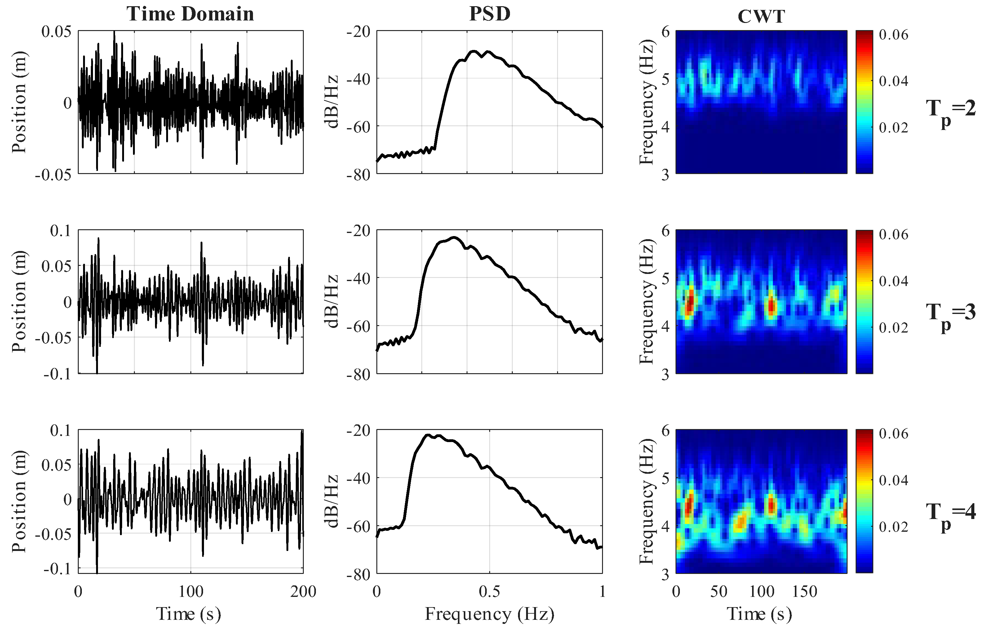
WEC parameters such as position (z), velocity ($\dot{z}$), and PTO force ($F_{\mathrm{PTO}}$) exhibit small variations in changing wave period ($T_p$). Traditional time-domain approaches, such as statistical moments or signal amplitude variations, are insufficient in differentiating rapid and subtle changes in $T_p$. Therefore, we incorporate frequency domain features and time–frequency representations to better capture variations in ocean wave dynamics.

The Continuous Wavelet Transform (CWT) is a powerful tool for analyzing non-stationary signals by providing a joint representation in both time and frequency domains. Unlike the Fourier Transform, which decomposes a signal into pure sinusoids without time localization, CWT utilizes wavelets—localized basis functions—to capture transient and localized frequency variations [20].

Mathematically, the CWT of a signal $x\left(t\right)$ is defined as

$$W(a,b)={\int }_{-\infty }^{\infty }x\left(t\right){\psi }_{a,b}^{*}\left(t\right)dt$$

(21)

where ${\psi }_{a,b}^{*}\left(t\right)$ is the scaled and translated version of the mother wavelet $\psi \left(t\right)$, given by

$${\psi }_{a,b}\left(t\right)={\displaystyle \frac{1}{\sqrt{\left|a\right|}}}\psi \left({\displaystyle \frac{t-b}{a}}\right)$$

(22)

Here, a represents the scale parameter, which controls the frequency resolution, and b is the translation parameter, which determines the time localization of the wavelet. The choice of the mother wavelet affects the resolution and sensitivity of the transform.

In this work, CWT is employed to extract time–frequency features from WEC measurements, enabling more accurate prediction of the wave period $T_p$. The wavelet coefficients $W(a,b)$ provide a multi-resolution analysis, capturing both high-frequency transient behavior and long-term variations. By integrating these features with the LSTM model, our system improves its ability to classify sea states despite small variations in $T_p$.

As shown in Figure 4, the first column presents the WEC position $z\left(t\right)$ in the time domain for different wave periods $T_p=2$, 3, and 4 s. The signals do not exhibit noticeable changes in amplitude or period at first glance. The second column displays the power spectral density (PSD), where a small variation in peak magnitude can be observed, particularly in the dominant frequency components. The third column represents the CWT-based time–frequency analysis, where distinct differences in wave energy distribution across time and frequency become evident. This highlights the advantage of using time–frequency representations in characterizing sea states, as CWT effectively distinguishes subtle changes in $T_p$ that are not apparent in conventional time or frequency domain analyses.

Several features are extracted from the WaveBot time-series data in the time domain and frequency domain. A list of features is shown in

Table 2. Selected top 10 features.

Feature	Significance	Mathematical Representation
Peak Frequency	The frequency corresponding to the maximum PSD.	${\displaystyle f_{\mathrm{peak}}=argmaxP\left(f\right)}$
Spectral Centroid	Center of mass of the power spectrum.	${\displaystyle f_{\mathrm{centroid}}=\frac{\sum fP\left(f\right)}{\sum P\left(f\right)}}$
Spectral Flatness	Ratio of geometric mean to arithmetic mean of the power spectrum.	${\displaystyle F_{\mathrm{flat}}=\frac{exp\left(\frac{1}{N}\sum lnP\left(f\right)\right)}{\frac{1}{N}\sum P\left(f\right)}}$
Spectral Entropy	Quantifies the uniformity of spectral energy distribution.	${\displaystyle H=-\sum P\left(f\right)logP\left(f\right)}$
Band Power	Power in low (0–1 Hz), mid (1–3 Hz), and high frequencies.	${\displaystyle {\int }_{f_{\mathrm{low}}}^{f_{\mathrm{high}}}P\left(f\right)df}$
Wavelet Entropy	Measures disorder in wavelet energy distribution.	${\displaystyle H_{\mathrm{wavelet}}=-\sum P\left(s\right)logP\left(s\right)}$
Dominant Wavelet Scale	Scale corresponding to highest wavelet energy.	${\displaystyle s_{\mathrm{dom}}=argmaxE\left(s\right)}$
Wavelet Skewness	Asymmetry of wavelet coefficients’ distribution.	${\displaystyle \frac{\sum {(W(s,t)-{\mu }_W)}^3}{{\sigma }_W^3}}$
Wavelet Kurtosis	Peakedness of wavelet coefficients’ distribution.	${\displaystyle \frac{\sum {(W(s,t)-{\mu }_W)}^4}{{\sigma }_W^4}}$
Teager Energy Operator	Captures localized energy variations in the signal.	${\displaystyle \sum _{n=2}^{N-1}{x}_n^2-x_{n-1}{x}_{n+1}}$

. To identify the n-best features from the WaveBot physical measurements, we introduce a composite z-score approach that integrates multiple feature evaluation metrics, providing a comprehensive measure of feature importance. Traditional feature selection methods often rely on a single criterion, which may overlook aspects of feature relevance or redundancy. Our composite z-score mitigates these limitations by combining multiple metrics, each capturing distinct aspects of feature importance.

The composite z-score for each feature i, denoted as $z_{\mathrm{composite},i}$, is defined as a weighted sum of normalized scores derived from multiple feature evaluation metrics. Let m be the number of feature evaluation methods included in the composite z-score, and let $z_{i,j}$ denote the normalized score for feature i under the j-th evaluation method. Then, the composite z-score for feature i is given by

$$z_{\mathrm{composite},i}=\sum _{j=1}^m{w}_j·z_{i,j}$$

(23)

where $w_j$ is the weight assigned to the j-th evaluation method, with ${\sum }_{j=1}^m{w}_j=1$. Each $z_{i,j}$ is normalized to ensure comparability across different methods and scales, typically by converting raw scores into z-scores based on the mean and standard deviation of the metric values for all features. This study uses three feature evaluation metrics to construct the composite z-score: Pearson correlation coefficient [21], variance threshold [22], and SHAP scores [23]. Each metric captures a unique aspect of feature relevance, with Pearson correlation measuring linear relationships, variance thresholding highlighting high-variance features, and SHAP scores providing model-agnostic importance based on feature contributions to predictions.

The scores from each metric are normalized to ensure comparability and then combined into a composite z-score using a weighted sum:

$$z_{\mathrm{composite},i}=w_1·z_{i,\mathrm{correlation}}+w_2·z_{i,\mathrm{variance}}+w_3·z_{i,\mathrm{SHAP}}$$

(24)

where $w_1$, $w_2$, and $w_3$ are weights assigned to each metric, with $w_1+w_2+w_3=1$. The weights are selected based on cross-validation performance to ensure optimal feature selection for our specific model and data.

After calculating $z_{\mathrm{composite}}$ for each feature, the top 10 features with the highest $z_{\mathrm{composite}}$ values are selected as the final feature set. This composite z-score approach demonstrates improved robustness and interpretability compared to single-metric feature selection as shown in our empirical results in Section 4.

5. Result Analysis

5.1. Model Training

In the first stage, the WaveBot device is simulated in MATLAB/Simulink (Version 24.1) to generate device position (z), velocity ($\dot{z}$), and PTO force ($F_{\mathrm{PTO}}$). A wide range of JONSWAP spectra is used to mimic real-life ocean conditions. Wave heights of $H_m\in [1,6]$ m and peak periods of $T_p\in [8,15]$ s are suitable for Pacific Northwest sea conditions. Therefore, a full-scale $T_p$ ranging from 1 to 15 s is used to generate the WaveBot physical data. Since we are using a 1/17th scaled version of the original WaveBot device, we apply similar scaling to the input wave characteristics, $H_m$ and $T_p$.

During training, wave excitation force, $F_{\mathrm{exc}}$ is generated using wave surface elevation profiles for $T_p\in [1,4]$ s, $H_m=0.127$ m, and the hydrodynamic properties of the WaveBot device. A time step of 0.01 s is used to generate device data that are later used to train the LSTM model. The choice of window size and step size in feature extraction plays a critical role in effectively capturing the underlying dynamics of the WEC. In this study, we select a sampling frequency of 100 Hz, meaning that each recorded second contains 100 data points. To ensure that the extracted features encapsulate meaningful temporal variations, a window size of 1000 samples is chosen, equivalent to 10 s of data per window. This 10-s duration is sufficiently long to capture the dominant wave characteristics and WEC response while balancing computational efficiency. Given that ocean waves exhibit characteristic periods ranging from a few seconds to over a dozen seconds, this window size ensures that at least one full wave cycle is included in each window, even for the longest wave periods in the dataset.

For model training, wave periods ($T_p$) between 1 and 4 s are used, covering a wide range of dynamically different sea states. In all cases, the wave height $\left(H_m\right)$ and the peak enhancement factor ($\gamma$) are fixed at 0.127 m and 1, respectively. We have used Python 3.10 along with TensorFlow 2.11.0 to build, train, and test the LSTM-based neural network model. A list of model architecture is shown in

Table 3. LSTM model architecture.

Parameter	Value
Loss Function	MSE
Optimizer	Adam
Number of Layers	2
Neurons per Layer	50, 50
Dropout	0.2
Batch Size	32
Epochs	50
Learning Rate	0.001
Activation Function	ReLU

.

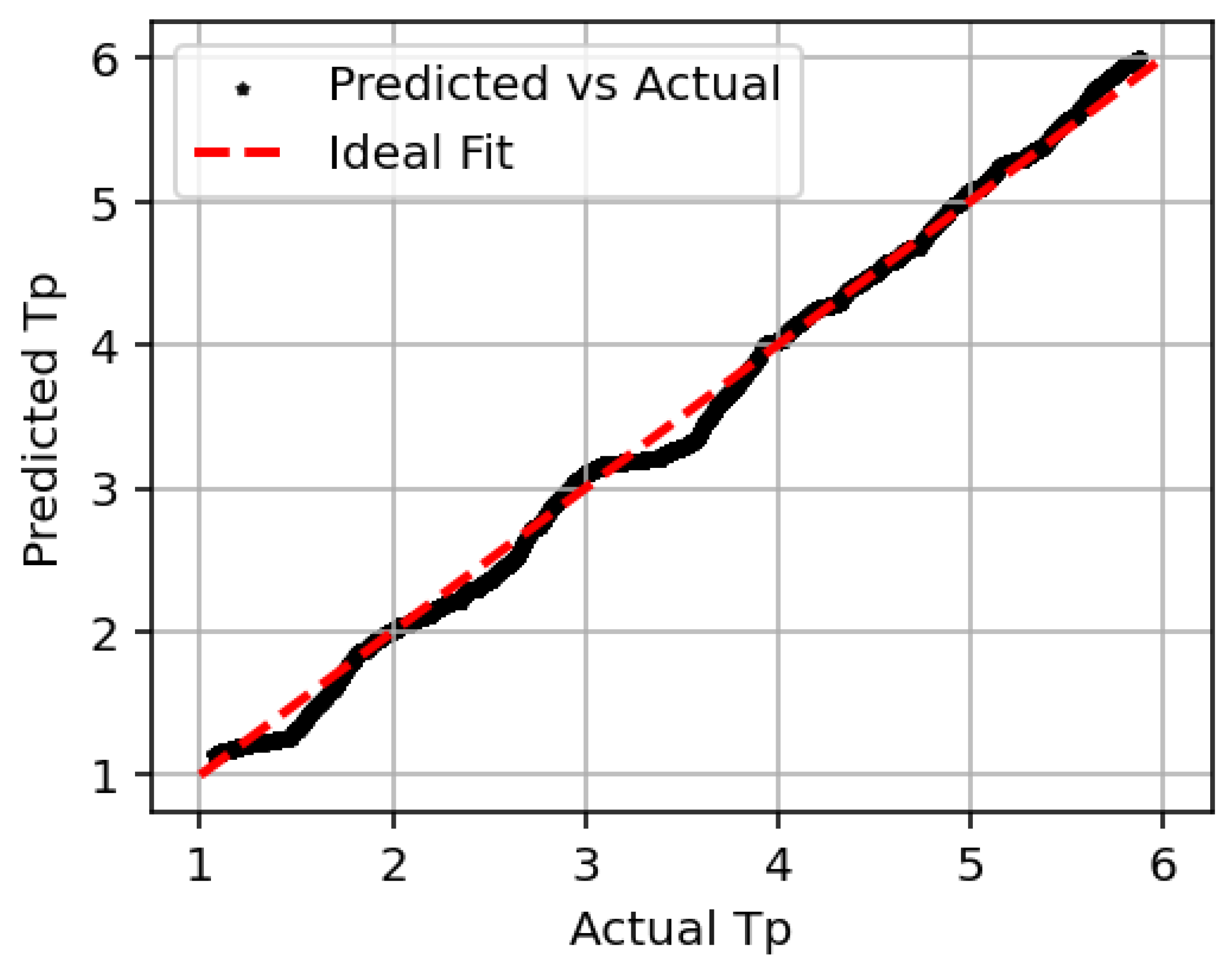
Figure 5 illustrates the comparison between predicted and actual peak period ($T_p$) values. The black scatter points represent the LSTM model’s predictions, while the red dashed line corresponds to the ideal one-to-one fit. The close alignment of most data points along this line indicates strong predictive performance. The model achieves a coefficient of determination ($R^2$-score) of 98.4%, demonstrating its ability to capture the underlying wave dynamics with high accuracy. Even on test data with $T_p$ values extending beyond the training range, the model maintains strong predictive capability, highlighting its generalization performance. Minor deviations from the ideal fit can be seen due to inherent noise in wave conditions and model uncertainties. However, the overall trend confirms that the LSTM-based approach effectively learns the nonlinear relationships between wave excitation forces and device responses, making it a reliable choice for real-world WEC applications.

5.2. Fixed Sea State: Prediction and Control

The trained LSTM model is employed within the control loop via MATLAB-Python co-design integration. As a supervisory control, the trained LSTM model predicts the incoming wave period, $T_p$, based on WaveBot measurements $(z,\dot{z},F_{\mathrm{PTO}})$, which is then used to determine and apply the proportional and integral gains $K_P$ and $K_I$. Predicted $T_p$ is normalized since Min-Max scaling is applied during training. Therefore, it is scaled back to its original form using the Min-Max values of the features.

Figure 6 and Figure 7 present the simulation results from MATLAB/Simulink, demonstrating the effectiveness of the trained LSTM model in real-time wave prediction, and control applied based on that prediction. The first subplot of Figure 6 shows the setting of the fixed period case, in which the control parameters are set based on the accurate prediction of a 5 s sea state, and the prediction of the sea state based on observations of the system response. The subsequent plots display the variations in control parameters, $K_P$ and $K_I$, which adapt dynamically based on the predicted $T_p$. Note that $K_I$ gain is limited to $-2\times {10}^4$ due to the device constraint as shown in Table 1. The position, velocity, and PTO force ($F_{\mathrm{PTO}}$) plots further illustrate the system’s response to the incoming waves. Figure 7 illustrates the average power captured over time for two control approaches.

The PTO power $P_{\mathrm{PTO}}\left(t\right)$ is computed using the instantaneous PTO force $F_{\mathrm{PTO}}\left(t\right)$ and the velocity of the device $\dot{z}\left(t\right)$. The instantaneous PTO power is given by

$$P_{\mathrm{PTO}}\left(t\right)=F_{\mathrm{PTO}}\left(t\right)·\dot{z}\left(t\right).$$

(25)

The average power $P_{\mathrm{avg}}$ is then computed by dividing the total extracted energy by the total time duration T:

$$P_{\mathrm{avg}}={\displaystyle \frac{1}{T}}{\int }_0^T{P}_{\mathrm{PTO}}\left(t\right)dt.$$

(26)

In conventional control strategies, $T_p$ remains constant, potentially limiting adaptability to changing wave conditions. In contrast, our approach updates $T_p$ every 10 s based on real-time responses from the WaveBot device. This adaptation leads to a more responsive control strategy, yielding improved power capture. The results show that the proposed method achieves an average power of 36.65 W, compared to 35.26 W with the fixed $T_p$, slightly improving power capture compared to the fixed $T_p$ approach.

5.3. Variable Sea State: Prediction and Control

The water surface elevation function $\eta \left(t\right)$ is constructed as

$$\eta \left(t\right)=\sum _{i=1}^N\sqrt{2S_c({\omega }_i,t)}sin({\omega }_{i}t+{\varphi }_i)$$

(27)

where ${\omega }_i$ is the angular frequency, ${\varphi }_i$ is a random phase uniformly distributed in $[0,2\pi ]$, and $S_c(\omega ,t)$ is the time-dependent wave spectrum transitioning between two sea states:

$$S_c(\omega ,t)={\displaystyle \frac{5{\pi }^4{H}_s{\left(t\right)}^2}{T_p{\left(t\right)}^4{\omega }^5}}exp\left({\displaystyle \frac{-20{\pi }^4}{T_p{\left(t\right)}^4{\omega }^4}}\right)$$

(28)

$$H_s\left(t\right)=m_1\left(t\right)H_{s1}+m_2\left(t\right)H_{s2},$$

(29)

$$T_p\left(t\right)=m_1\left(t\right)T_{p1}+m_2\left(t\right)T_{p2},$$

(30)

where the time-dependent mixing coefficients are given by

$$m_1\left(t\right)=1-{\displaystyle \frac{t}{t_{\mathrm{end}}}},m_2\left(t\right)={\displaystyle \frac{t}{t_{\mathrm{end}}}}.$$

(31)

This ensures a smooth transition from sea state 1 at $t=0$ to sea state 2 at $t=t_{\mathrm{end}}$. The resulting wave elevation function $\eta \left(t\right)$ accurately represents a dynamically evolving sea state.

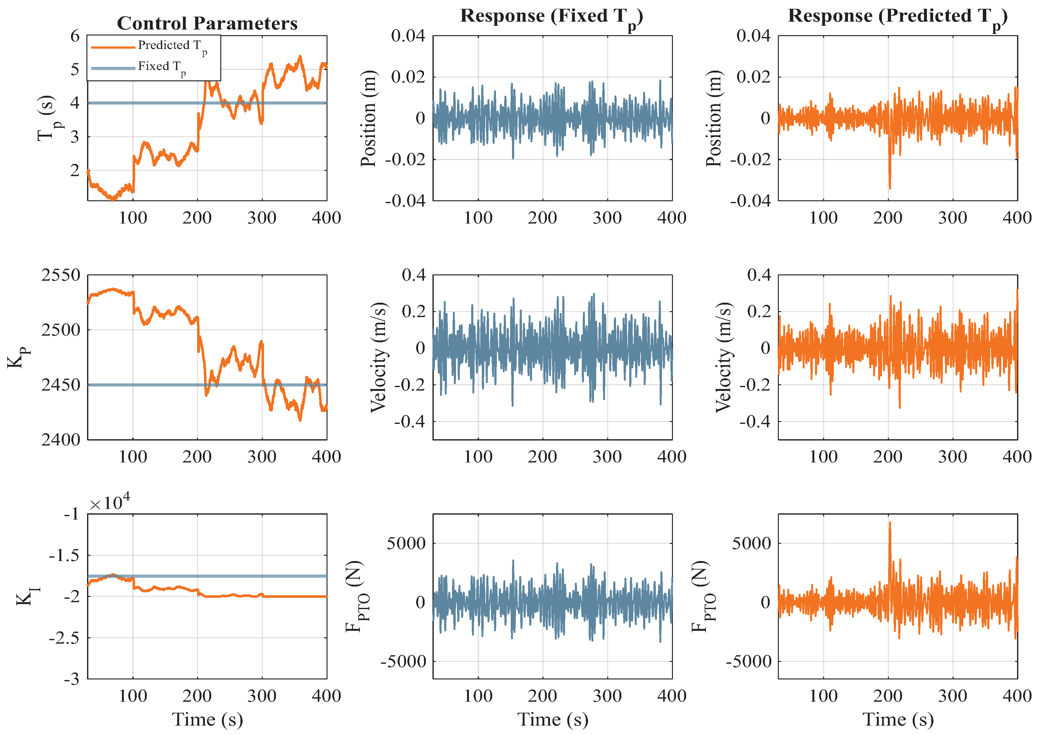
Figure 8 presents the WEC motion response under a dynamically varying wave period $T_p$ ranging from 2 s to 6 s. The left column displays the control parameters: the estimated period $T_p$, proportional gain $K_P$, and integral gain $K_I$, while the right column illustrates the WaveBot device response in terms of position, velocity, and PTO force over time. In the first column, it is evident that the predicted period approach is tracking the changing sea state and adjusting the proportional and integral gains accordingly.

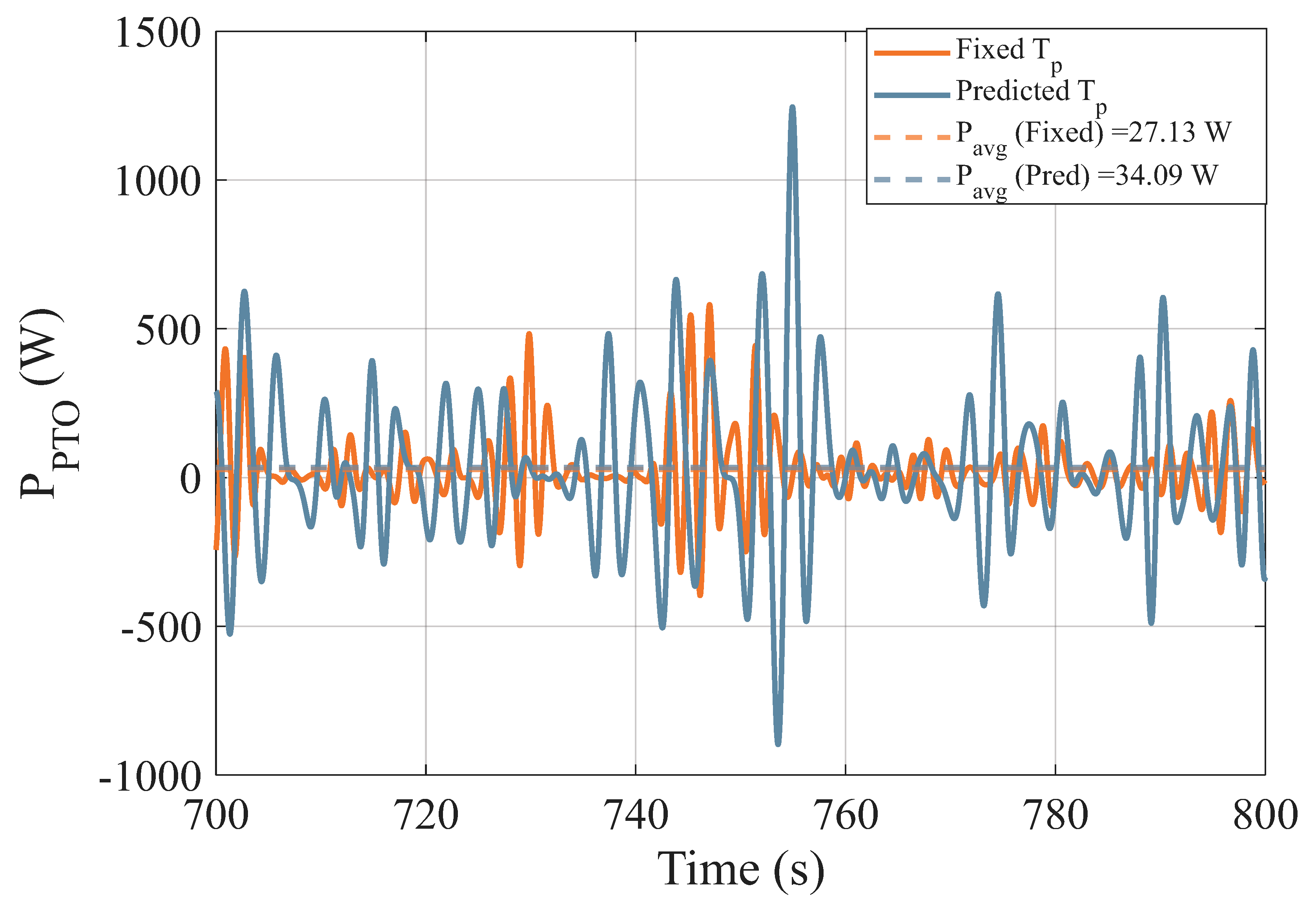
Figure 9 illustrates the average power capture over time for two control approaches: a fixed $T_p$ of 4 s (conventional method) and a dynamically predicted $T_p$. Unlike the fixed approach, where $T_p$ remains constant, the proposed method adaptively updates $T_p$ based on real-time responses from the WaveBot device, enabling the continuous tuning of the proportional gain $K_P$ and integral gain $K_I$. The results demonstrate a significant improvement in power capture with the adaptive approach. The proposed method achieves an average power of 34.09 W, compared to 27.13 W with the fixed $T_p$. This demonstrates a 25.6% increase in power capture compared to the fixed $T_p$ approach. This increase in power extraction efficiency is attributed to the real-time adjustment of control parameters, which allows the WEC to better synchronize with incoming wave conditions. By dynamically optimizing $K_P$ and $K_I$, the system effectively maximizes energy conversion, validating the advantage of adaptive control over traditional fixed-gain strategies.

6. Discussion

Our proposed control approach is compared with several other traditional machine learning models and control strategies.

Table 4. Comparison of different models for fixed and variable $T_p$.

Model	Fixed ${\mathit{T}}_{\mathit{p}}$			Variable ${\mathit{T}}_{\mathit{p}}$
	${\mathbf{R}}^{\mathbf{2}}$-Score	RMSE	Pavg (W)	${\mathbf{R}}^{\mathbf{2}}$-Score	RMSE	Pavg (W)
ANN	0.95	0.02	35.6	0.92	0.04	33.11
SVR	0.89	0.09	34.21	0.87	0.15	31.86
LSTM	0.98	0.005	36.65	0.96	0.03	34.09
Baseline (PI)	-	-	35.26	-	-	27.13

presents a comparative analysis of different models for both fixed and variable $T_p$, emphasizing the effectiveness of the proposed LSTM-based control technique. The results demonstrate that LSTM outperforms ANN and SVR across all performance metrics, achieving the highest $R^2$-score and the lowest RMSE for both cases. For the fixed $T_p$ scenario, LSTM attains an $R^2$-score of 0.98 with an RMSE of 0.005, leading to an average power capture ($P_{\mathrm{avg}}$) of 35.26 W, the highest among all models. Similarly, under the variable $T_p$ approach, LSTM maintains superior performance with an $R^2$-score of 0.96 and an RMSE of 0.03, achieving an average power capture of 34.09 W. This power capture outperforms the baseline PI controller, which yields 27.13 W. The key outcome of this study is the demonstrated effectiveness of the LSTM-based control approach in adapting to varying sea states. Conventional PI control with fixed $K_P$ and $K_I$ struggles with dynamic wave conditions, showing similar power capture in fixed sea states but poor performance in variable sea states. However, the proposed method dynamically adjusts control parameters, leading to enhanced power extraction. These results validate the potential of machine learning-driven adaptive control strategies in optimizing energy capture for wave energy converters. The proposed LSTM model demonstrates promising results in predicting ocean wave parameters from WaveBot measurements; however, certain limitations remain. One of the major challenges is the MATLAB-Python co-design integration, which requires specific version compatibility for both training and testing phases. Also, the addition of AWGN to the WaveBot measurements can cause discrepancies, especially at peak force amplitudes; hence, the model’s sensitivity to noise intensity requires further investigation.

Future work could address these limitations by exploring alternative noise models, such as colored noise, to better simulate oceanic environments. Additionally, we plan to leverage direct CWT images as inputs to train CNNs for improved feature extraction and wave parameter predictions. Pretrained CNN models will also be explored to enhance the accuracy and efficiency of $T_p$ estimation, leveraging transfer learning techniques for better generalization across varying sea states. Furthermore, integrating the model with real-time data acquisition from WaveBot could provide insights into practical implementation challenges and further optimize performance for live ocean energy applications. Addressing these directions would improve the model’s robustness, generalizability, and practical value in ocean wave prediction and energy harvesting.

7. Conclusions

This study presented an LSTM-based approach for predicting sea states by utilizing features extracted from a WEC device’s physical measurements. Later, a MATLAB-Python co-design architecture is used to integrate wave predictions with a PID controller to obtain optimal control actions that maximize energy extraction. The results show that the proposed control approach significantly enhances power capture in both fixed and variable sea conditions. For the fixed sea state case, the proposed method captures the same amount of power as the traditional fixed $T_p$ approach, which is optimally tuned for that particular $T_p$. In the variable sea state scenario, the model was able to tune PID controller gains based on the real-time wave conditions. This adaptation improved power capture by 25.6%, demonstrating the effectiveness of the real-time tuning of $K_p$ and $K_i$ using the LSTM-predicted sea states. By leveraging these improvements, our proposed method can offer a practical, resilient solution for WEC control by focusing on device measurements, thereby reducing the need for complex and costly wave predictions.