Abstract
The safe management of traffic on rail networks requires that trains can be reliably located at all times. In many countries, this is achieved by electrically identifying their presence using ‘track circuits’ at regular intervals along each track: these devices detect when the wheels and axles of a train short-circuit the two rails (they are said to ‘shunt’ them) and the information is passed on to the signaling system. The quality of the electrical contacts between the rails and the wheels obviously plays a decisive role in the correct operation of this detection principle. The occurrence of high wheel–rail contact resistances can lead to malfunctions, known as ‘deshunting’, in which the system is unable for a certain period of time to conclude whether a train is present or absent on a section of track. This type of potentially risky event must obviously be avoided at all costs. In this article, we present the second part of a study devoted to the degradation of the wheel–rail contact resulting from steel oxidation, using a scaled-down home-made test bench that reproduces the real contact in the laboratory under controlled conditions. Following on from the first part, which dealt with the static characterization of the contact studied in the direct current, we are now tackling its dynamic characterization (rolling contact) under AC electrical conditions close to those of a track circuit. These new investigations again involve different degrees of rail oxidation, and analyze the influence of parameters such as contact force, speed, and current intensity.
1. Introduction
The real-time information about the presence of a train in a specific track section is realized by a “track circuit” system and is paramount to avoid hazardous situations. It ensures the accurate localization of the train on the railway and hence the track safety as shown in Figure 1. When the train is absent, the signal sent by the transmitter reaches the receiver via the transmission line. In this situation, the residual is generally close to the circuit’s supply voltage. On the contrary, the presence of a train axle on the track creates a low resistance, known as a shunt, which “short-circuits” the two rails, causing the residual voltage to drop “to zero”. This is referred to as “shunting”. When the residual voltage falls below a certain threshold, indicating the occupancy of the zone, the signaling systems are activated accordingly.
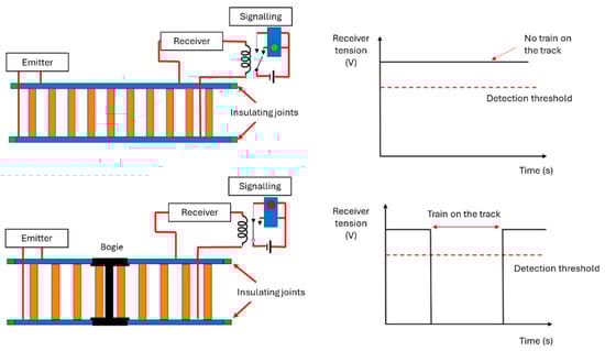
Figure 1.
Operating principle of a track circuit and the ideal residual voltage profile. (Top): No train present on the track. (Bottom): Track occupied by an axle, indicating a prohibited passage.
A high-quality electrical contact must be maintained for ensuring the reliability of the track circuit system. A high impedance of the contact spot leads to a critical safety issue, known as “deshunting”, in which, for a certain period, the train is no longer detected. As already pointed out in the very recent study focusing on wheel-rail contact in static conditions [1], it is well known that among several sources of pollution that can modify the contact resistance, thin oxide layers can play a major role, especially on tracks with low frequentation. Even though various devices to prevent [2,3] or reduce the occurrence of deshunting have been implemented, many instances are still detected every year.
Consequently, there is a need to better understand the behavior of the wheel rail electrical contact of a rolling stock to design fault resistant railway management strategies intending to avoid potentially dangerous situations (level crossing failures, rail accidents, etc.).
Wheel–rail contact is a complex, multi-physical subject since it involves both mechanical and electrical aspects. In [4,5,6], the detection and impact of the mechanical degradation of the wheel and the rail were studied. Parameters related to the surface, such as roughness [7,8], local temperature, and physical chemistry [9], were shown to have a strong influence on the wheel–rail contact resistance. In certain instances, arcing has been observed to occur between the wheel and the rail, resulting in microstructural modifications of the surfaces [7,10]. The state of the surfaces and the inherent complexities of its multi-physical character are not exclusive to the two solids in contact, but also extend to a layer referred to as a “third body” present at their interface. This third body has been found to contain a wide variety of components, including wear particles from wheels and rails, external contaminants, such as dead leaves, frost, sand, and oil, as well as rust formed naturally on the surfaces [11]. Such components can potentially affect the friction at the interface [12,13]. In [14], the tribological, morphological, and microscopic properties of third body samples were examined and their electrical conductivity, heterogeneity, and compactness were compared between good and bad shunting conditions.
Railway maintenance is significantly impacted by rust, particularly in coastal or humid regions where corrosion is known to be more severe. Rainwater can deposit salts or atmospheric contaminants, resulting in the formation of acidic rain which accelerates the corrosion process [15]. Suzumura et al. studied the rust composition by using in situ X-ray diffraction [16]. On the railhead, they mainly found FeO(OH) oxyhydroxides in various forms and Fe3O4 magnetite. Taking a step back from these considerations, Fukuda et al. [17] examined how the type of track environment and how often trains pass affect the rust thickness on rails and the wheels roughness. Using a huge test bench involving real wheel and rail elements, they also studied how various factors, such as normal load, current intensity, and oxide layer thickness, affect contact resistance.
Subsequent studies conducted in parallel on a 1/4 scale test bench and on site with an instrumented regional train, both stationary and running at low speed, have further refined the understanding of the wheel–rail electrical contact [18,19]. These studies demonstrated that the results obtained at a reduced scale are fully representative of those obtained at full scale. This important observation validated the relevance of working on a scaled-down model to facilitate the study of the influence of the many possible parameters (load force, imposed current intensity, surface properties, rolling speed, etc.). Consequently, the authors recently developed a flexible experimental device to accurately replicate the wheel–rail contact conditions in the laboratory, along with a protocol to achieve different oxidation states on demand [20]. It is this versatile platform allowing studies on a much smaller scale than those previously proposed that is used in the present work. As has been demonstrated in the literature, the presence of rust causes non-linear current–voltage characteristics [21,22]. Therefore, the subject of oxidation was the primary focus of the experimental platform, with initial emphasis placed on the simplest cases of static contact and direct current stresses [23]. In order to more accurately reflect the context of rail traffic, new investigations are reported hereafter, based on a series of tests conducted using rolling conditions and alternating current. The work presented in this paper is the follow up work of this previous publication.
This paper will therefore focus on the influence of a controlled thickness oxide layer on the wheel/rail contact resistance under dynamic conditions, to better understand its non-ohmic behavior and with the application aim of estimating the maximum admissible rust state of a railway track. The measurements were carried out under reproducible conditions (speed, load, and oxidation state) on our reduced-scale bench. They required the development of specific analysis tools, mainly based on statistical analysis, to obtain the maximum information on the electrical behavior of the wheel/rail contact. After a brief reminder of the structure and implementation of the bench, these new tools will be detailed before presenting the results obtained.
2. Experimental Setup and Tests Conditions
The setup described in [20] consists in a reduced-scale wheel running on a 1 m full-scale rail. The mechanical laws were considered in order for the scaled-down wheel to be representative of the full-scale behavior of the wheel–rail contact. The aspect ratio of the contact surfaces as well as the average contact pressure at both scales are maintained. The applied normal force on the wheel axis is controlled with an electrical actuator, and the pressure on the contact is dimensioned so as to be equivalent to that produced by a real loaded train. In this paper the sizing of the scaled-down wheel—a roller—was designed to mimic the real wheel of a train of interest used on the French rail network (FRN). For clean, smooth, and fully conductive surfaces subjected to a normal force F = 400 N (corresponding to a force of 77 kN/wheel for the real train mimicked), the elliptical contact area half-axes were calculated as and .
The measurement of the wheel–rail electrical contact resistance is performed using the four-point method, as shown in the diagram in Figure 2, which illustrates the principle of this technique applied to the test bench. Two copper thread brushes are used to inject the current from a source into the contact, while two other brushes, placed closest to the contact, are used to measure the contact voltage. The current flowing through the contact is evaluated by measuring the voltage across a well-known resistor.
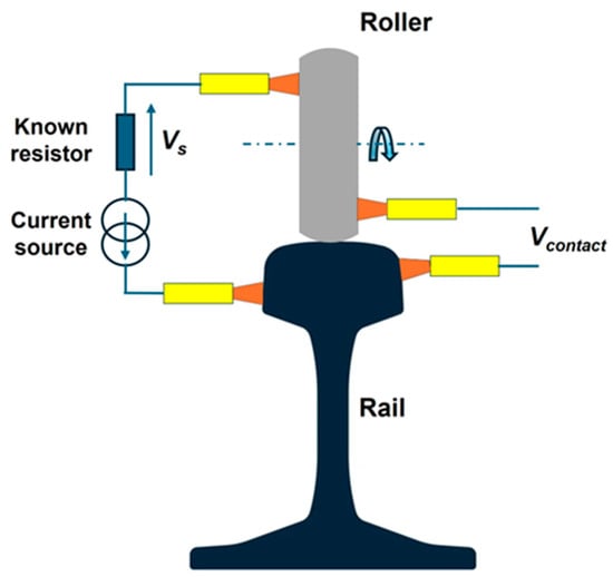
Figure 2.
Schematic of the electrical measurement setup on the bench, based on the four-point method.
The dynamic test series presented in the following Section 4.1 and Section 4.2 examine the influence on the contact resistance of the following parameters: degree of oxidation, current intensity, applied normal force, and displacement speed. In the case of oxidation, two main surface conditions were considered. On the one hand, a reference case, known as “clean”, where a distinction was made between a surface cleaned a few days prior, still shiny, upon which a microscopic oxide layer of unquantifiable thickness had begun to appear, and a surface freshly stripped just before testing, very shiny. These two facies were implemented on 1 m-long rail sections, which can be seen in Figure 3a. On the other hand, a case formed by ‘light’ oxidations, is intended to describe the situation of tracks with low daily traffic and unfavorable environmental conditions. For these facies, we segmented another 1m rail into three zones, each about 30 cm long (zones L1, L2, and L3), with different levels of oxidation, as illustrated in Figure 3b. These zones have average oxide thicknesses of about 4 μm, 12 μm, and 8 μm, respectively, based on 30 thickness measurements on each (see Table 1). The surfaces were oxidized by vaporizing a 0.6 mol/L aqueous solution of NaCl on the rail. The degree of oxidation was controlled by changing the open-air drying time (respectively 15, 45, and 30 min) at ambient temperature.
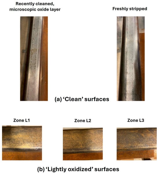
Figure 3.
Photographs of studied rail surfaces. (a) ‘Clean’ surfaces: with a microscopic oxide layer (left) and freshly stripped (right). (b) ‘Lightly oxidized surfaces’: three zones with different oxide thicknesses.

Table 1.
Oxide thickness (mean value and standard deviation) for each zone.
In the tests, the roller was moved along the rail at controlled speed and normal force. A sinusoidal current of three different amplitudes at a frequency of (typical of the UM71 track circuit type) was injected into the contact. For each current intensity, two distinct forces were applied: and . For each of these forces, two different speeds were tested: and . An incremental encoder mounted on the roller hub enables its position to be known at all times, through a voltage signal , and electrical measurements to be synchronized with zones of interest on the rail. The evolution of electrical signals as a function of time is captured using a LeCroy WaveRunner 625zi oscilloscope associated to a ZD1500 active differential probe (equipment from Teledyne LeCroy, Courtaboeuf, France).
3. Analytical Methods
3.1. Statistical Representation of Voltage/Current Characteristics
In order to observe the electrical behavior of the roller–rail contact, we used a statistical representation of current/voltage values proposed in previous studies [18]. This approach makes it possible to deduce the quality of the contact from the observation of the voltage–current characteristics (linearity, dominant resistance, maximum voltage reached, etc.).
For this purpose, synchronized time measurements of (, , and ) are captured and organized into three-column matrices with rows, where each row corresponds to a combination of , , and
The next step is to use the signal of position sensor to isolate the time segments directly linked to the movement of the roller in the zone of interest on the rail. These segments are then processed to exclude saturated periods when the voltage reaches the compliance of the current source (Keithley 6221 DC/AC Current Source, equipment from Tektronix, Les Ulis, France), which is as illustrated in Figure 4.
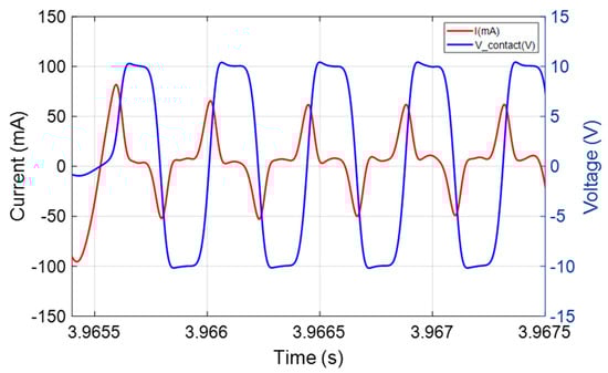
Figure 4.
Example of a chronogram showing possible strong distortions in the current signal (-) associated with saturation of the contact voltage (-), reaching the compliance of the current source.
The data is then used to create statistical maps illustrating the current–voltage relationship. The method consists in discretizing the contact voltage and current signals with steps and and estimating the density of occurrence of the different pairs Figure 5 shows an example of this representation: the horizontal axes represent the two parameters and , and the vertical axis represents the density of occurrence, with a color scale where red represents the highest density. This density is expressed in logarithmic scale and corresponds to the number of points obtained in each discretization cell of dimensions . An adjustment of +1 is applied to all occurrence densities to avoid values of zero (for which the logarithm would not be defined).
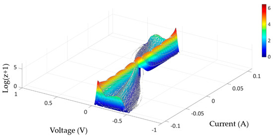
Figure 5.
Example of a statistical representation of a set of voltage–current characteristics. Areas of discretization are shown on the graph by gray lines.
For tests on oxidized rail, the current and voltage ranges were set at and for current, and and for voltage. This selection reflects the maximum current injected during testing, set at . For clean rail testing, the same current ranges were applied, while the voltage limits were and , which include extreme voltage values reached during clean rail testing. These limit values were used to discretize the current–voltage space and to normalize the mappings.
For fine resolution of the characteristics , the current–voltage space has been segmented into 401 × 401 zones. The discretization is adapted according to the condition of the rail analyzed: for oxidized rails, the dimensions are ; whereas, for clean rails, they are reduced to . In fact, this differentiation offers greater finesse in the resolution of low voltages on clean rails. The probability density for each zone was then normalized by the total number of measurements.
One can notice that the characteristic is nonlinear. As outlined in [1], at the outset of a current cycle, the contact resistance is elevated due to the presence of the oxide film at the interface. As the current flows, localized Joule heating raises the temperature at the asperities [24], which in turn modifies the oxide layer and lowers its electrical resistivity [25]. Simultaneously, the hardness of both the steel and oxide diminishes with the increasing temperature [26]. Together, these factors broaden the real contact zone by causing breaks in the oxide film and compressing asperities, thereby enhancing metal-to-metal contacts.
Once the current is further increased, the reduction in contact resistance begins to level off, indicating a slower progression in the contact’s evolution. An interpretation of this phenomenon has been proposed based on an electro-thermal process in granular media (the Branly effect) [27,28]. This effect describes an evolution of the contact resistance that is initially reversible, then progressively irreversible, due to changes in the numerous contacts present within the granular medium.
3.2. Estimation of ‘Main Resistance’ from U-I Data
In all our statistical representations of the voltage–current data we have identified a dominant contact resistance (in red) which we call the ‘main resistance’. To estimate this resistance, we have developed a method that consists in determining the equation of the straight line connecting the voltage–current pairs with the highest densities of occurrence. This technique involves examining the statistical maps to identify in two specific current ranges , one positive and the other negative, the pair (U, I) located in each current interval and representing the highest density of occurrence. We then simply draw the straight line that passes through these two specific points on the map. The slope of this straight line corresponds to the main resistance.
To standardize our approach independently of the currents applied, we have defined and , as shown in Figure 6.
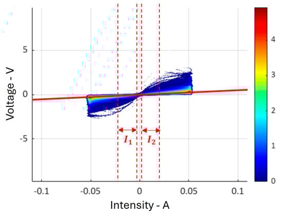
Figure 6.
Illustrative example of estimation of the main resistance from the U–I data, illustrated by the thick red line. In the intervals I1= [−21 mA; −5 mA] and I2 = [5 mA; 21 mA], the most frequent (U, I) pairs determine the main resistance, represented by the slope of this line.
This method has made it possible to examine the influence of various parameters such as maximum current intensity, applied force and speed on this main contact resistance.
3.3. Statistical Analysis of Instantaneous Resistances
To estimate the continuous variations in the contact resistance due to the contact surface alterations encountered during movement, we have calculated the instantaneous resistance according to Equation (1):
where and are respectively the voltage and current measured at each sampling time. It is therefore possible to monitor variations in contact resistance over extremely short time intervals, of the order of microseconds, corresponding to the oscilloscope sampling frequency of 1 MHz.
If the roller moves over a long rail section at a speed of we obtain measurements of . Thanks to this large data set, it is possible to evaluate the variations in contact resistance observed during dynamic testing. To this end, statistical analyses have been carried out on this dataset, identifying the median and interquartile range (IQR). The median gives an indication of the central value of the resistance, while the IQR, as shown in Figure 7, is an indicator of the data homogeneity. It is calculated as the difference between the 25th percentile and the 75th percentile of all values. The higher the IQR width, the greater the dispersion of resistances.
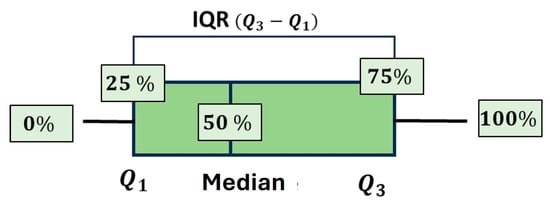
Figure 7.
Box plot illustrating the median and IQR (interquartile range) for a dataset.
On a clean rail surface, the median value is generally low and the IQR is reduced, reflecting more homogeneous resistance values. However, on a less clean surface, the median increases and the IQR widens, indicating more dispersed resistance values.
Figure 8 shows an example of the graphical representation of these statistical measurements (median and IQR) as a function of the current, for different applied forces and speeds. This method can therefore be used to quantitatively evaluate the electrical behavior of the wheel–rail contact for different operating conditions through statistical analysis of instantaneous resistances. It enables trends in characteristics to be detected, and to identify the critical parameters that have a significant influence on the contact behavior.

Figure 8.
Schematic diagram of the graphical representation of statistical measurements—(•) Median and (I) IQR—of contact resistances for different current intensities.
4. Dynamic Testing
4.1. Clean Rail
4.1.1. Clean Rail: Statistical Mapping of the U-I Characteristics
For each of the two surfaces presented in Figure 3a, we have drawn up statistical distributions of the current–voltage characteristics. These maps are shown in Figure 9 and Figure 10. The maximum voltage values reached are of the order of ±0.5 V. We see a predominantly linear main trend, surrounded by less frequent, non-linear, and scattered features. For the rail with microscopic oxidation, the effects of current intensity and speed on resistance are less noticeable. However, an effect of applied force is perceptible: the voltage–current characteristics become less dispersed at 400 N than at 200 N. For freshly stripped rail, it is difficult to draw any conclusion on the basis of these maps.
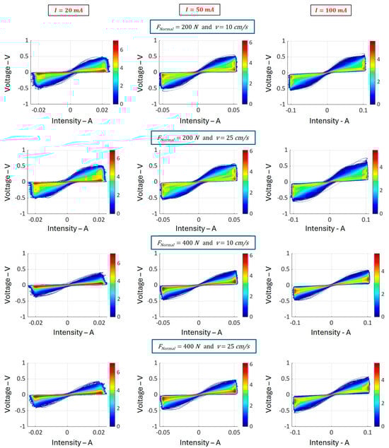
Figure 9.
Statistical maps of current–voltage characteristics obtained for the recently cleaned rail, for different current intensities (20 mA, 50 mA, and 100 mA, with f = 2300 Hz), forces (200 N and 400 N), and speeds (10 cm/s and 25 cm/s).
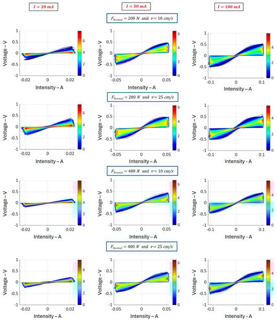
Figure 10.
Statistical maps of current–voltage characteristics obtained for the freshly stripped rail before testing, for different current intensities (20 mA, 50 mA, and 100 mA, with f = 2300 Hz), forces (200 N and 400 N), and speeds (10 cm/s and 25 cm/s).
4.1.2. Clean Rail: Statistical Analysis of Instantaneous Resistances
We then proceed to the statistical analyses of the instantaneous resistances, which are presented in Figure 11. For each ‘clean’ rail considered, we have calculated the median and IQR for the different experimental conditions. These data are then plotted as a function of current intensity.
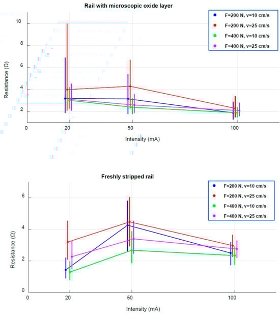
Figure 11.
Statistical analysis of contact resistances R(t) obtained for the two ‘clean’ rails as a function of current intensity, showing median values of contact resistances (•) and their IQR intervals (I).
For the recently cleaned rail with a microscopic oxide layer, the effect of current is noticeable: whatever the speed and force applied, IQRs are wider at 20 mA than at 50 mA or 100 mA. The voltage–current characteristics therefore become less dispersed as the current intensity increases. What is more, in most cases, with the exception of , and , the median tends to decrease with the increasing current, and the contact resistance decreases with the increasing force.
As the statistical maps also show, a force effect is clearly visible, with lower IQR widths at than at , independently of current and speed. The voltage–current characteristics tend to be less dispersed with the increasing force.
The effect of velocity, less perceptible in distribution maps, becomes evident through a statistical analysis of R(t). As speed increases, irrespective of the intensity injected and the force considered, the median and IQR width tend to increase. Contact resistance tends to increase and the voltage–current characteristics tend to be more dispersed with the increasing speed.
For the freshly stripped rail, the force and velocity effects correspond to those observed on the surface with a microscopic oxide layer. However, the variation as a function of intensity shows an unexpected trend: resistance increases during the transition from to , then decreases at 100 mA. This may seem paradoxical. It could be attributed to a thermal effect induced by the current, sufficient to cause an increase in the resistivity of the metal (steel), but not sufficient for the softening of the material to contribute to a decrease in resistance. The effect should be more or less the same for 100 mA, since the maximum voltages are of the same order. However, for this current value, a decrease in resistance is observed.
To validate these observations, we repeated the experiment under the same conditions, stripping the rail again. We noted an identical trend at , where the contact resistance reaches its maximum values. At present, we have no explanation for this.
4.2. Light Oxidation
Using the same protocol as before, we studied the case of “light” oxidation on the different rail zones, identified as L1, L2, and L3, as shown in Figure 3b (their thickness values and standard deviations are reported in Table 1).
4.2.1. Light Oxidation: Statistical Mapping of the U-I Characteristics
For each of these zones, we have drawn up statistical representations of the current–voltage characteristics, as shown in Figure 12, Figure 13 and Figure 14 under different test conditions.
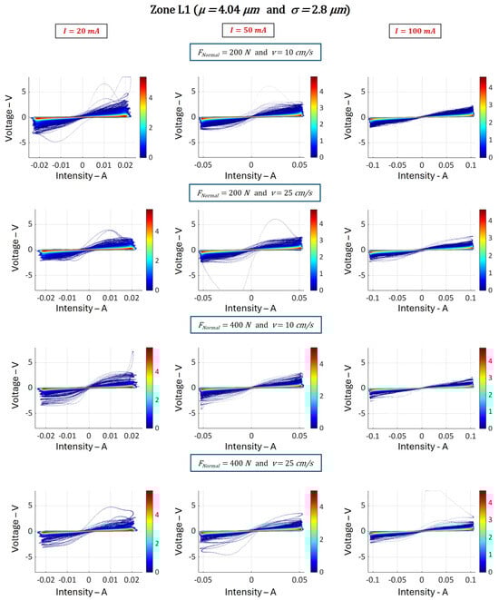
Figure 12.
Statistical maps of current–voltage characteristics obtained on zone L1, with an average oxide thickness of 4 μm, for different current intensities (20 mA, 50 mA, and 100 mA, at f = 2300 Hz), forces (200 N and 400 N), and speeds (10 cm/s and 25 cm/s).
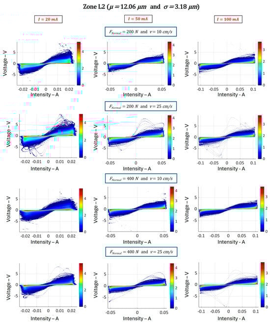
Figure 13.
Statistical maps of current–voltage characteristics obtained on zone L2, with average oxide thickness 12.1 μm for different current intensities (20 mA, 50 mA, and 100 mA, at f = 2300 Hz), forces (200 N and 400 N), and speeds (10 cm/s and 25 cm/s).
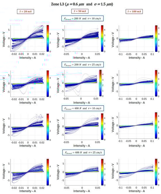
Figure 14.
Statistical maps of current–voltage characteristics obtained on the L3 zone, with an average oxide thickness of 8.6 μm, for different current intensities (20 mA, 50 mA, and 100 mA, at f = 2300 Hz), forces (200 N and 400 N), and speeds (10 cm/s and 25 cm/s).
Overall, the results show high resistance characteristics. Maximum voltages reach 5 V (or even more).
In all these statistical representations, we note a predominant main characteristic, marked in red, which shows a linear behavior. All around, other less frequent characteristics can be observed. They are non-linear, dispersed, and highly resistant. Characteristic dispersion and maximum voltage values increase with oxide thickness.
These maps also allow us to conclude the following:
- The majority of the dominant voltage–current characteristics (in red) observed are linear, which confirms the results of previous studies conducted by SNCF and GeePs [18,19]. These studies showed that the characteristics remain linear as long as the current does not exceed .
- The effect of current is noticeable:
- (i)
- This trend is reflected in a decrease in the maximum voltages reached as the current increases.
- (ii)
- Increasing current also tends to reduce the dispersion of characteristics.
- However, the effects of force and speed are less obvious to evidence from these data.
Anomalies can be observed in certain maps. An example is shown in Figure 15 (upper part, red box). This map corresponds to measurements obtained in zone L3 with a current intensity of 20 mA at a force of 200 N and a speed of 10 cm/s. It shows the presence of certain pairs of points (U, I) in quadrants 2 and 4. This means that there are situations where the current I is positive while the voltage U is negative, or vice versa. These singularities could be explained either by the presence of noise in the signal, as shown by the chronograms presented in the lower part of Figure 15 (circled in red), or by the existence of a significant phase shift between I and U. Such anomalies remain relatively infrequent in relation to the total number of periods considered.
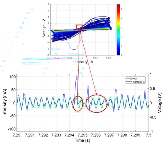
Figure 15.
Examples of singularities in the U-I maps (framed in red). (Top): map from test on zone L3 with I = 20 mA, F = 200 N and v = 25 cm/s. (Bottom): extracts from the U(t) and I(t) time signals illustrating these singularities (circled in red).
4.2.2. Lignt Oxydation: Statistical Analysis of Instantaneous Resistances
The results of the statistical analysis of instantaneous resistances are shown and plotted against the current in Figure 16. For each zone considered, we calculated the median and interquartile range (IQR) of resistance values R(t) under the different experimental conditions. Several interesting conclusions can be drawn as follows:
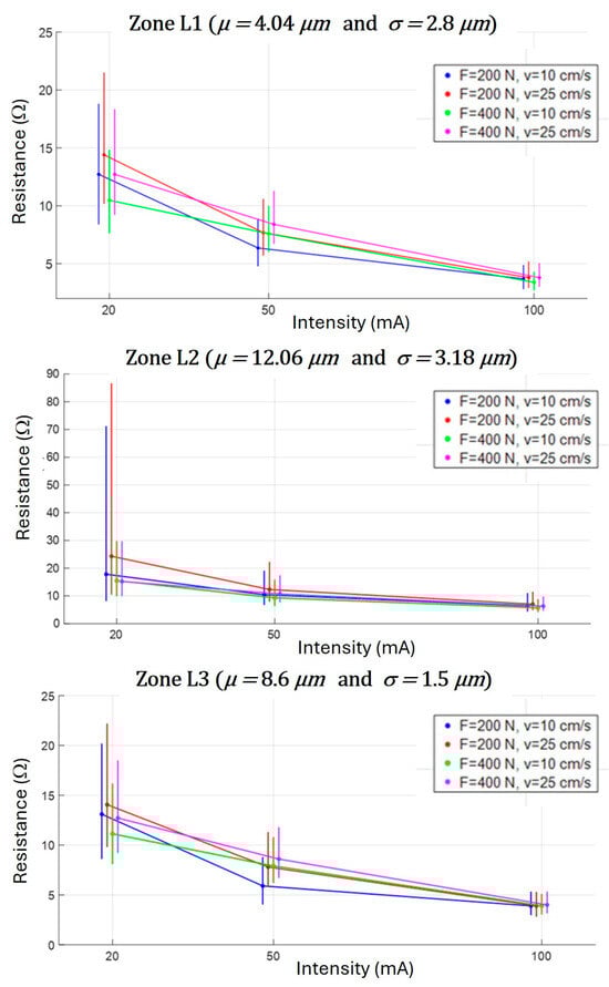
Figure 16.
Representation of statistical analyses of contact resistances R(t) obtained for different oxide thicknesses (4 μm, 12.06 μm, 8.6 μm) as a function of current intensity, showing median values of contact resistances (•) and their IQR intervals (I).
- Effect of oxide thickness: Resistance tends to increase with oxide thickness. In particular, zone L2, which has a thicker oxide layer than the other two zones, shows particularly high resistance values, up to around , especially for low currents (). On the other hand, zones L1 and L3, with thinner oxide layers, show resistances relatively close to each other under all test conditions, and well below those recorded for zone L2.
- Current effect:
- (i)
- Resistance tends to decrease with the increasing current intensity, irrespective of oxide thickness and test conditions. The median decreases with the increasing intensity, a trend also observed in statistical maps. In zones L1 and L3, resistance decreases gradually from around at to approximately at . In zone L2, resistance is reduced from at to around at .
- (ii)
- Dispersion of the voltage–current characteristics is reduced with the increasing current. This is also observed in the statistical maps.
- (iii)
- As the current intensity increases, the effect of force and speed on contact resistance becomes less pronounced.
This result underlines the fact that current is a key determining factor influencing contact resistance more than any other experimental parameter.
- Effect of force: as force increases, the contact resistance tends to decrease and the voltage–current characteristics are less dispersed. This can be attributed to an increase in the number of asperities coming into contact and a widening of the contact zones, mainly due to the flattening of asperities under the effect of pressure.
- Effect of speed: as speed increases, the contact resistance tends to rise and the voltage–current characteristics become more dispersed. In fact, increasing speed leads to accelerated renewal of the contact surface, thus reducing the number and size of asperities involved.
5. Conclusions
Using the versatile scaled-down experimental set-up presented in previous papers, we investigated the electrical behavior of the wheel–rail contact under dynamic conditions and with alternating current at 2.3 kHz for various rail surface states and operating conditions. The article highlights three specific analysis tools that have been developed to interpret the test results: statistical representation of the voltage–current characteristics, estimation of the dominant characteristic, and statistical analysis of the instantaneous resistance R(t) based on the median and IQR.
Experiments were carried out for various oxidation states, values of current intensity, applied force, and speed. The main trends observed can be summarized as follows:
- -
- Force: as force increases, the resistance and dispersion of the voltage–current characteristics tend to decrease.
- -
- Speed: as speed increases, the resistance and dispersion of the voltage–current characteristics tend to increase.
- -
- Current intensity: for lightly oxidized rail sections, as the current intensity increases, contact resistance and dispersion tend to decrease; for ‘clean’ rail sections, the effect of the current is less pronounced.
- -
- Oxidation: contact resistance tends to increase with oxide thickness. This was expected, but it is important to note that it can also be affected by the temperature of the contact point, which can dramatically increase due to the current flowing through small contact spot.
For the future, we plan to develop an approach that will enable us to simulate the detection of bad shunting, still on the reduced-scale bench. This would be achieved by introducing both a detection threshold on the contact voltage and also the equivalent of a time delay, the key point being the dimensioning of these two parameters to be representative of the reality of track circuits.
Author Contributions
Conceptualization, F.L., F.H. and P.T.; methodology, L.H., F.L., F.H. and P.T.; software, L.H. and F.L.; validation, F.L., F.H. and P.T.; formal analysis, L.H., F.L., F.H. and P.T.; investigation, L.H., F.L., F.H. and P.T.; resources, K.S. and F.G.; data curation, L.H.; writing—original draft preparation, L.H., F.L., F.H. and P.T.; writing—review and editing, F.L., F.H., K.S., F.G. and P.T.; visualization, L.H., F.L., F.H., K.S., F.G. and P.T.; supervision, F.L., F.H., K.S., F.G. and P.T.; project administration, F.L., F.H., K.S., F.G. and P.T.; funding acquisition, F.L., F.H. and P.T. All authors have read and agreed to the published version of the manuscript.
Funding
This research was funded by the Société Nationale des Chemins de Fer français (SNCF), the French National Railway Network.
Data Availability Statement
The data are not publicly available due to privacy restrictions.
Conflicts of Interest
The authors declare no conflicts of interest.
References
- Haydar, L.; Loete, F.; Houzé, F.; Slimani, K.; Guiche, F.; Testé, P. Influence of the oxide layer thickness on the behavior of the electrical wheel-rail contact in static conditions. Appl. Sci. 2025, 15, 471. [Google Scholar] [CrossRef]
- Na, L.; Cai, B.; Zhang, C.; Liu, J.; Li, Z. A heterogeneous transfer learning method for fault prediction of railway track circuit. Eng. Appl. Artif. Intell. 2025, 140, 109740. [Google Scholar] [CrossRef]
- Peng, F.; Liu, T. Method for Fault Diagnosis of Track Circuits Based on a Time–Frequency Intelligent Network. Electronics 2024, 13, 859. [Google Scholar] [CrossRef]
- Mosleh, A.; Montenegro, P.A.; Costa, P.A.; Calçada, R. Railway Vehicle Wheel Flat Detection with Multiple Records Using Spectral Kurtosis Analysis. Appl. Sci. 2021, 11, 4002. [Google Scholar] [CrossRef]
- Mosleh, A.; Montenegro, P.; Alves Costa, P.; Calçada, R. An approach for wheel flat detection of railway train wheels using envelope spectrum analysis. Struct. Infrastruct. Eng. 2021, 17, 1710–1729. [Google Scholar] [CrossRef]
- Wei, Y.; Han, J.; Yang, T.; Wu, Y.; Chen, Z. Research on wheel/rail contact surface temperature and damage characteristics during sliding contact of a wheel. J. Eng. Appl. Sci. 2024, 71, 201. [Google Scholar] [CrossRef]
- Li, J.; Zhang, Y.; Zhao, B.; Zheng, Z. Research and Analysis on Contact Resistance of Wheel and Insulated Rail Joint in High-Speed Railway Stations. Electronics 2023, 12, 1272. [Google Scholar] [CrossRef]
- Ren, W.; Zhang, C.; Sun, X. Electrical Contact Resistance of Contact Bodies with Cambered Surface. IEEE Access 2020, 8, 93857–93867. [Google Scholar] [CrossRef]
- Itagaki, M.; Nozue, R.; Watanabe, K.; Katayama, H.; Noda, K. Electrochemical impedance of thin rust film of low-alloy steels. Corros. Sci. 2004, 46, 1301–1310. [Google Scholar] [CrossRef]
- Al-Juboori, A.; Zhu, H.; Wexler, D.; Li, H.; Lu, C.; Azdiar; Gazder, A.; McLeod, J.; Pannila, S.; Barnes, J. Microstructural changes on railway track surfaces caused by electrical leakage between wheel and rail. Tribol. Int. 2019, 140, 105875. [Google Scholar] [CrossRef]
- Descartes, S.; Desrayaud, C.; Niccolini, E.; Berthier, Y. Presence and role of the third body in a wheel–rail contact. Wear 2005, 258, 1081–1090. [Google Scholar] [CrossRef]
- White, B.; Lewis, R.; Fletcher, D.; Harrison, T.; Hubbard, P.; Ward, C. Rail-wheel friction quantification and its variability under lab and field trial conditions. Proc. Inst. Mech. Eng. Part F J. Rail Rapid Transit 2024, 238, 569–579. [Google Scholar] [CrossRef]
- Broster, M.; Pritchard, C.; Smith, D.A. Wheel/rail adhesion: Its relation to rail contamination on british railways. Wear 1974, 29, 309–321. [Google Scholar] [CrossRef]
- Descartes, S.; Renouf, M.; Fillot, N.; Gautier, B.; Descamps, A.; Berthier, Y.; Demanche, P. A new mechanical-electrical approach to the wheel-rail contact. Wear 2008, 265, 1408–1416. [Google Scholar] [CrossRef]
- Xu, W.; Zhang, B.; Deng, Y.; Wang, Z.; Jiang, Q.; Yang, L.; Zhang, J. Corrosion of rail tracks and their protection. Corros. Rev. 2021, 39, 1–13. [Google Scholar] [CrossRef]
- Suzumura, J.; Sone, Y.; Ishizaki, A.; Yamashita, D.; Nakajima, Y.; Ishida, M. In situ X-ray analytical study on the alteration process of iron oxide layers at the railhead surface while under railway traffic. Wear 2011, 271, 47–53. [Google Scholar] [CrossRef]
- Fukuda, M.; Terada, N.; Ban, T. Study of quantifying and reducing electrical resistance between wheels and rails. Q. Rep. RTRI 2008, 49, 158–162. [Google Scholar] [CrossRef]
- Chollet, H.; Houzé, F.; Testé, P.; Loete, F.; Lorang, X.; Debucquoi, S. Observation of Branly’s effect during shunting experiments on scaled wheel-rail contacts. In Proceedings of the 9th International Conference on Contact Mechanics and Wear of Rail/Wheel Systems (CM2012), Chengdu, China, 27–30 August 2012; pp. 111–114. [Google Scholar]
- Houzé, F.; Chollet, H.; Testé, P.; Lorang, X.; Loëte, F.; Andlauer, R.; Debucquoi, S.; Lerdu, F.; Antoni, M. Electrical behaviour of the wheel-rail contact. In Proceedings of the 26th International Conference on Electrical Contacts (ICEC-ICREPEC2012), Beijing, China, 14–17 May 2012; pp. 67–72. [Google Scholar]
- Haydar, L.; Loete, F.; Houzé, F.; Choupin, T.; Guiche, F.; Testé, P. Enhancing Railway Network Safety by Reproducing Wheel–Rail Electrical Contact on a Laboratory Scale. Appl. Sci. 2023, 13, 10253. [Google Scholar] [CrossRef]
- Kaza, G.-L.; Houzé, F.; Loëte, F.; Testé, P. Experimental Study and Phenomenological Laws of Some Nonlinear Behaviours of the Wheel–Rail Contact Associated with the Deshunting Phenomenon. Appl. Sci. 2023, 13, 11752. [Google Scholar] [CrossRef]
- Holm, R. Electrical Contacts: Theory and Applications, 4th ed.; Springer: Berlin, Germany, 2000. [Google Scholar]
- Duvivier, P.-Y. Étude Expérimentale et Modélisation du Contact Electrique et Mécanique Quasi Statique Entre Surfaces Rugueuses d’or: Application aux Micro-Relais MEMS. Ph.D. Thesis, Ecole Nationale Supérieure des Mines de Saint-Étienne, Saint-Étienne, France, 2010. [Google Scholar]
- Kim, W.; Wang, Q.J. Numerical Computation of Surface Melting at Imperfect Electrical Contact between Rough Surfaces. In Proceedings of the 52nd IEEE Holm Conference on Electrical Contacts, Montréal, QC, Canada, 25–27 September 2006; pp. 81–88. [Google Scholar]
- Puech, L. Élaboration et Caractérisations de Couches Minces de Magnétite pour des Applications Microbolométriques. Ph.D. Thesis, Université Toulouse 3 Paul Sabatier, Toulouse, France, 2009. [Google Scholar]
- Huang, Y.-S.; Chen, L.; Lui, H.-W.; Cai, M.-H.; Yeh, J.-W. Microstructure, Hardness, Resistivity and Thermal Stability of Sputtered Oxide Films of AlCoCrCu0.5NiFe High-Entropy Alloy. Mater. Sci. Eng. A 2007, 457, 77–83. [Google Scholar] [CrossRef]
- Falcon, E.; Castaing, B. Electrical conductivity in granular media and Branly’s coherer: A simple experiment. Am. J. Phys. 2005, 73, 302–307. [Google Scholar] [CrossRef]
- Dorbolo, S.; Ausloos, M.; Vandewalle, N. Reexamination of the Branly effect. Phys. Rev. E 2003, 67, 040302. [Google Scholar] [CrossRef] [PubMed]
Disclaimer/Publisher’s Note: The statements, opinions and data contained in all publications are solely those of the individual author(s) and contributor(s) and not of MDPI and/or the editor(s). MDPI and/or the editor(s) disclaim responsibility for any injury to people or property resulting from any ideas, methods, instructions or products referred to in the content. |
© 2025 by the authors. Licensee MDPI, Basel, Switzerland. This article is an open access article distributed under the terms and conditions of the Creative Commons Attribution (CC BY) license (https://creativecommons.org/licenses/by/4.0/).