First-Arrival Constrained Physics-Informed Recurrent Neural Networks for Initial Model-Insensitive Full Waveform Inversion in Vertical Seismic Profiling

Abstract

FWI is a nonlinear optimization problem; significant discrepancies between the initial and true velocity models can lead to solutions converging to local optima. To address this issue, we proposed a PIRNN-based FWI method with first-arrival time constraints. Physics-informed recurrent neural networks (PIRNNs) integrate the physical processes of seismic wave propagation into recurrent neural networks, offering a novel approach for full-waveform inversion (FWI). First, the physical processes of seismic wave propagation were embedded into the recurrent neural network, enabling finite-difference solutions of the wave equation through forward propagation. Second, first-arrival time differences between synthetic and observed records were calculated, which then guided the selection of appropriate seismic traces for FWI loss computation. Additionally, the spatiotemporal gradient information recorded during the forward propagation of the recurrent neural network was utilized for backpropagation, enabling nonlinear optimization of FWI. This method avoids the local optima caused by waveform mismatches between the observed and synthetic records resulting from inaccurate initial velocity models. Numerical experiments on the BP and Marmousi velocity models demonstrated that the proposed method accurately reconstructed subsurface velocity structures even when the initial model significantly deviated from the true model, and maintained a degree of reconstruction accuracy in the presence of considerable noise, thereby validating its low sensitivity to the initial model and its robustness against noise.

1. Introduction

Seismic exploration plays a pivotal role in various geoscientific and resource exploration applications, offering invaluable insights into the Earth’s subsurface structures. Modern seismic surveys typically involve generating controlled seismic energy at or near the surface and recording the resulting wavefields with an array of receivers. The recorded data subsequently undergo rigorous processing to enhance signal quality and prepare them for seismic inversion. Seismic inversion aims to deduce quantitative models of subsurface physical parameters, such as seismic velocity, from these surface observations. Among the array of inversion techniques, Full-Waveform Inversion (FWI) has garnered significant attention due to its potential for yielding high-resolution subsurface images. FWI is a method for obtaining detailed subsurface medium parameters and was first proposed by Tarantola [1]. The primary goal of this inversion is to minimize data misfit between observed and synthetic seismic waveforms to derive an optimal subsurface medium parameter model [2]. However, FWI typically requires a reasonably accurate initial estimate of the subsurface parameters. A starting model that is close to the true subsurface velocity structure is a prerequisite for a successful FWI [3]. This prerequisite is necessary because FWI data generation is largely based on the wave equation, where the medium parameters are integral to the equation [4]. When the initial medium parameters deviate significantly from the true subsurface structure, the inversion tends to converge to local optima, leading to inaccurate results. Therefore, the initial model is a critical factor that directly influences inversion results, and constraints must be applied during FWI to reduce its dependency.

In traditional FWI, there are two approaches for processing the initial model. The first step involves estimating the initial model using the observed data. For example, conventional tomography methods and travel time information can generate relatively accurate initial models for FWI [5], followed by full-waveform inversion. Although this approach has been applied successfully, it relies on low-frequency information to ensure the accuracy of the initial model. When this information is missing, it is challenging to provide a sufficiently accurate initial FWI model. The second approach focuses on improving the inversion process to reduce dependency on the initial model. For example, multiscale methods [6] divide the FWI problem by frequency, starting with lower frequencies to capture large-scale subsurface structures and then transitioning to higher frequencies for finer details. Although this method mitigates nonlinearity to an extent, it depends on low-frequency information found within the data, which is challenging to obtain through field surveys. In addition, improper frequency-band partitioning can affect the resolution of the model. Another method involves expanding the optimization search space [7] to avoid local minima by incorporating the wave equation constraint as a regularization term in the objective function. This approach significantly broadens the search space and reduces dependency on the initial model. However, relaxing the physical constraints of the wave equation may lead to results that do not fully satisfy physical laws, thereby compromising accuracy. Similarly, adding regularization terms, such as total variation regularization [8], can constrain the solution space and reduce dependency on the initial model. However, this approach may lead to over smoothing and requires careful parameter tuning. Another approach modifies the FWI objective function by focusing on the observed and synthetic data. Traditional FWI minimizes the squared difference between the observed and synthetic data, but the oscillatory nature of seismic data results in numerous local minima. Alternative methods include using matched filters [9] for trace-by-trace matching and employing optimal transport distances [10,11] or envelope-based misfits [12,13]. Although these methods reduce dependency on the initial model, they cannot guarantee accurate results when the initial model is of poor quality.

In recent years, deep learning has gained traction in scientific and engineering fields, offering new solutions to complex geophysical problems, particularly in seismic inversion [14]. Traditional deep learning-based FWI is typically data-driven [15,16], indicating that its effectiveness depends on the size and quality of the seismic dataset. Without constraints from geophysical forward modeling, traditional FWI results lack physical interpretability. To address this limitation, researchers have begun to integrate physics-informed neural networks (PINNs) with FWI to introduce physical constraints. PINNs, first proposed by Raissi et al. [17], solve nonlinear partial differential equations and have shown promise in seismology research. For example, Rasht-Behesht et al. [18] proposed a mesh-free FWI method using PINNs for wave-equation solutions. Sun et al. [19] developed a theory-guided system that incorporates wave equation physics into a network training loop using a physics-driven data misfit as a loss function to enhance interpretability. Although PINN-based methods reduce the dependence of FWI on the initial model by introducing physical constraints, challenges remain in practical applications owing to limited prior information and data acquisition constraints. To address these challenges, Du et al. [20] proposed an implicit FWI (IFWI) using PINNs for seismic forward modeling. Their method employs a deep neural network (DNN) that emphasizes low-frequency learning, significantly reducing dependency on the initial model; however, its effectiveness depends substantially on the design of the deep learning model. Another approach involves leveraging neural networks to directly parameterize or generate the velocity model. For example, Zhu et al. [21] proposed a neural-network-based FWI (NNFWI) where a generative neural network is used to represent the velocity model. This method capitalizes on the neural network’s ability to naturally introduce spatial correlations, acting as a regularization that helps suppress noise in the gradients and mitigate local minima, proving effective even for high-contrast structures and in the presence of noise. Furthermore, an alternative approach involves dynamic data matching, which enhances the correspondence between synthetic and observed data, thereby reducing dependency on the initial model. For instance, Zhou et al. [22] developed a full-waveform inversion technique centered on dynamic data matching of convolutional wavefields, employing one-dimensional Gaussian convolutional kernels to extract multi-scale features from individual time samples within seismic traces; these features are then used to identify optimally matched pairs between the observed and synthetic data. Utilizing first-arrival information to constrain FWI or improve the initial model is also an effective strategy. Some studies have focused on the joint inversion of travel time and waveform data [23,24], leveraging their respective strengths to constrain the model. In recent years, deep learning has been applied to first-arrival picking to enhance picking efficiency and accuracy, indirectly aiding FWI [25,26,27]. While these methods alleviate the initial model problem to some extent, how to effectively utilize first-arrival information to dynamically guide the waveform inversion process and integrate it with PIRNNs remains a direction worthy of further investigation.

In this study, we aim to reduce the impact of the initial model on FWI. Accordingly, we proposed a self-correlation progressive FWI method based on PIRNNs. The core novelty of this work is the synergistic integration of a first-arrival time constrained dynamic trace selection strategy with a Physics-Informed Recurrent Neural Network (PIRNN) framework, enabling the effective resolution of cycle skipping and a reduction in initial model dependency, all performed within a physically consistent deep learning architecture.

Specifically, the aims of our research were as follows:

(1)

Propose an initial velocity model-insensitive FWI method that effectively addresses the local minima caused by different initial velocity models.

(2)

Develop a PIRNN architecture with first-arrival time constraints by embedding the physical processes of seismic wave propagation into the recurrent neural network; through leveraging the spatiotemporal gradient information from forward propagation, this method enables back propagation under first-arrival constraints, thereby producing FWI solutions.

(3)

Introduce a knowledge-constrained neural network framework for FWI to avoid the instability issues of data-driven methods caused by the training data quality.

2. Problem Analysis and Theory

This section first analyzes the root causes of nonlinearity in FWI, particularly the cycle-skipping issue linked to initial model inaccuracies. Subsequently, it establishes the theoretical foundations for our proposed first-arrival constrained Physics-Informed Recurrent Neural Network (FAFWI-PIRNN) method, detailing the relevant FWI mathematics, first-arrival constraint mechanisms, and PIRNN principles.

2.1. Math Model of FWI

The goal of an FWI is to determine model parameters that minimize the difference between the synthetic seismic response and actual observed data. Typically, this optimization problem can be expressed as follows [1,2]:

$$m_{\mathrm{opt}}=\underset{\mathrm{m}}{\arg \min } J_D(m),$$

(1)

where $\mathbf{m}$ represents the model parameter vector and $J_D$ is the objective function that measures the difference between the observed data and synthetic data. To quantify this difference, the ${\mathrm{L}}_2$ norm is typically used as follows:

$$J_D={\displaystyle \sum _{s=1}^{N_s}{\displaystyle \sum _{t=1}^T\Vert d_{\mathrm{obs}}(}}{x}_r,x_s,t;m)-d_{\mathrm{cal}}(x_r,x_s,t;m_0){\Vert }^2,$$

(2)

where ${\mathbf{d}}_{\mathrm{o}\mathrm{b}\mathrm{s}}$ is the observed data, ${\mathbf{d}}_{\mathrm{c}\mathrm{a}\mathrm{l}}$ is the simulated data calculated using the initial model, ${\mathrm{m}}_0$, ${\mathrm{x}}_{\mathrm{r}}$, and ${\mathrm{x}}_{\mathrm{s}}$ represent the receiver and source positions, respectively, ${\mathrm{N}}_{\mathrm{s}}$ is the total number of sources, and T is the number of time steps. The $\left|\right|\cdot |{|}^2$ operator denotes the squared ${\mathrm{L}}_2$ norm, which calculates the sum of the squared differences between the elements of the enclosed data residual vector. The synthetic data are derived by solving the wave equation using numerical methods, and the observation system employed is vertical seismic profiling (VSP). VSP is an important geophysical exploration technique that requires placing receivers in a borehole to record seismic signals from the surface or borehole sources [28]. This method can produce high-resolution images of subsurface structures. Compared to conventional surface seismic exploration, VSP offers a higher resolution and signal-to-noise ratio, capturing more signals reflected from subsurface media and providing more accurate time-depth relationships and velocity information [29]. In FWI, VSP data can provide near-wellbore data or logging velocity as prior information, helping to reduce the dependence on the initial model [30].

To minimize the objective function $J_D$ (Equation (2)), it is necessary to compute its gradient with respect to the model parameter m. The gradient calculation formula is given as follows:

$${\displaystyle \frac{\partial J_D}{\partial m}}=-2{\displaystyle \sum _{s=1}^{N_s}{\displaystyle \sum _{t=1}^T{\left(\frac{\partial d_{\mathrm{cal}}(x_r,x_s,t,m)}{\partial m}\right)}^{\top }}}\left(d_{\mathrm{obs}}(x_r,x_s,t)-d_{\mathrm{cal}}(x_r,x_s,t,m)\right),$$

(3)

After computing the gradient, a suitable optimization algorithm was employed to update the model parameters based on the gradient. Commonly used optimization algorithms included the conjugate gradient and Newton’s methods. Once the direction and step size for the update were determined according to the selected optimization algorithm, the model parameters were updated using the following rule:

$$m^{k+1}=m^k-{\alpha }_k{\displaystyle \frac{\partial J_D}{\partial m}},$$

(4)

where ${\alpha }_k$ is the step size parameter computed by the optimization algorithm. The above process describes the traditional FWI workflow, in which the model parameters are iteratively updated to minimize the objective function until convergence is achieved, ultimately yielding the final FWI subsurface medium results.

2.2. Causes of Nonlinearity in FWI

A FWI is associated with an inherently highly nonlinear optimization problem. This nonlinearity renders the FWI solution highly sensitive to the initial model [31]. Specifically, when the initial model deviates significantly from the true model, the inversion process is prone to becoming trapped in the local minima, leading to results that diverge from the true solution. Figure 1 [3] demonstrates the cause of this phenomenon, where (b) represents the observed data of a seismic trace, and (a) and (c) represent the synthetic data of the corresponding trace generated through forward modeling using the initial model. In (a), the time delay $\Delta t$ between the $\mathrm{n}$-th cycle of the signal and the $\mathrm{n}$-th cycle of the observed data in (b) exceeds half a period ($\mathrm{T}/2$). In this case, the FWI matches the $\left(\mathrm{n}+1\right)$-th cycle of the signal in (a) with the $\mathrm{n}$-th cycle of the observed data in (b), causing the model update to proceed in the wrong direction. Further iterations lead to error accumulation, ultimately resulting in an incorrect model. In contrast, in (c), the time delay $\Delta t$ between the $\mathrm{n}$-th cycle of the signal and the $\mathrm{n}$-th cycle of the observed data in (b) is less than $\mathrm{T}/2$, allowing FWI to perform correct matching and model updates.

Therefore, combining with Equation (2), assuming the time delay between the observed data ${\mathbf{d}}_{\mathrm{o}\mathrm{b}\mathrm{s}}\left(t\right)$ and the synthetic data ${\mathbf{d}}_{\mathrm{c}\mathrm{a}\mathrm{l}}\left(t,\mathrm{m}\right)$ is $\Delta t$, the nonlinearity problem of FWI can be described as follows:

$$d_{\mathrm{cal}}(t,m)\approx d_{\mathrm{obs}}(t+\Delta t),$$

(5)

where $\Delta t$ is the time delay in seismic records caused by model errors. When $\Delta t<\mathrm{T}/2$, the waveforms of observed and synthetic data are aligned in time, and the objective function has a global minimum at $\Delta t=0$ (Figure 1c). The gradient points in the correct direction of the time delay enabled FWI to perform accurate matching and model updates. When $\Delta t>{\displaystyle \frac{\mathrm{T}}{2}}$, multiple local minima appeared in the parameter space of the objective function $J_D\left(\mathrm{m}\right)$, such as at $\Delta t=\mathrm{T}$, ${\displaystyle \frac{3}{2}}\mathrm{T}$, $2\mathrm{T}$, and so on (Figure 1a). The gradient pointing in the incorrect direction causes FWI to incorrectly match ${\mathbf{d}}_{\mathrm{c}\mathrm{a}\mathrm{l}}\left(t+nT,\mathrm{m}\right)$ with ${\mathbf{d}}_{\mathbf{o}\mathbf{b}\mathbf{s}}\left(t\right)$. This phenomenon is known as cycle-skipping. After skipping the cycle, the gradient function corresponding to Equation (3) becomes the following:

$${\displaystyle \frac{\partial J_D}{\partial m}}=-2{\displaystyle \sum _{s=1}^{N_s}{\displaystyle {\int }_0^T{\left(\frac{\partial d_{\mathrm{cal}}(t+\Delta t,m)}{\partial m}\right)}^{\top }}}\left(d_{\mathrm{obs}}(t)-d_{\mathrm{cal}}(t+\Delta t,m)\right)dt,$$

(6)

where ${\mathbf{d}}_{\mathrm{o}\mathrm{b}\mathrm{s}}\left(t\right)$ represents the observed data and t is the time variable. The synthetic data are denoted as ${\mathbf{d}}_{\mathrm{c}\mathrm{a}\mathrm{l}}\left(t+nT,\mathrm{m}\right)$, where $\Delta t$ represents the time delay and $\mathrm{m}$ represents the model parameters. The partial derivative of synthetic data with respect to the model parameters is expressed as ${\displaystyle \frac{\partial {\mathbf{d}}_{\mathrm{c}\mathrm{a}\mathrm{l}}\left(t+\Delta \mathrm{t},\mathbf{m}\right)}{\partial \mathbf{m}}}$. Additionally, ${\mathrm{N}}_{\mathrm{s}}$ represents the total number of sources and $\mathrm{T}$ represents the number of time samples. The direction of the gradient is jointly determined by two key factors: first, the residual between observed and synthetic data ${\mathbf{d}}_{\mathrm{o}\mathrm{b}\mathrm{s}}\left(t\right)-{\mathbf{d}}_{\mathrm{c}\mathrm{a}\mathrm{l}}\left(t+\Delta t,\mathbf{m}\right)$, and second, the sensitivity of synthetic data to model parameters ${\displaystyle \frac{\partial {\mathbf{d}}_{\mathrm{c}\mathrm{a}\mathrm{l}}\left(t+\Delta \mathrm{t},\mathbf{m}\right)}{\partial \mathbf{m}}}$. In conclusion, the time delay caused by the initial model directly determined whether the optimization process can converge to the global optimum.

2.3. Mitigating Nonlinearity Using First-Arrival Constraints

To address the cycle-skipping problem in FWI waveform matching, we introduced first-arrival constraints to mitigate this nonlinearity. Taking P-waves as an example, the first arrival is the earliest seismic wave to reach the receiver during wave propagation. Generally, the first arrival time occurs near the point of maximum energy in the seismic trace. Figure 2a shows an observed seismic record from a near-offset shot in a Vertical Seismic Profiling (VSP) system with dimensions $\mathrm{T}\times \mathrm{N}$, where $\mathrm{T}$ represents the sampling time and $\mathrm{N}$ represents the number of receivers. Figure 2b shows the synthetic seismic record from the initial model for the same near-offset shot. Performing FWI in this situation would lead to the cycle-skipping problem (Figure 1), causing the model updates to become trapped in the local optima. Therefore, these traces should be temporarily excluded from the loss calculation, whereas traces that satisfy the condition of first-arrival time differences of less than half a period should be included in the loss calculation and participate in model updates.

The First Arrival Constraint Strategy, in the initial stages of inversion, primarily focuses on selecting seismic traces where the first-arrival time difference ($\Delta t$) is less than or equal to half a period. These selected traces are then used to construct and optimize the objective function, ensuring accuracy and reliability in the inversion process. This strategy avoids the cycle-skipping phenomenon in FWI, thereby guiding the model parameters to iterate and update in the correct direction. Notably, this method does not directly use first arrivals for inversion; rather, it screens observed and synthetic seismic traces based on the constraint $\Delta t<\mathrm{T}/2$. The selected seismic traces remain complete, retaining both the first arrival and subsequent reflection information. Taking traces 5 and 50 from Figure 2 as examples, Figure 3a,b display seismic records that satisfy and fail to meet the time threshold condition, respectively. $\Delta t$ is quantified through calculating cross-correlation functions (Figure 3c,d). For case (a), because $\Delta t$ is less than half a period and the observed record contains rich wavefield information (including first arrivals and subsequent reflections), high-quality waveform matching can occur. In contrast, in case (b) where $\Delta t$ exceeds half a period, including these traces in the inversion calculation can lead to cycle-skipping problems and local minima; therefore, they are temporarily excluded during the initial stages of inversion. As the model parameters were iterated and optimized, the number of seismic records satisfying the first arrival time difference threshold condition gradually increased. This approach provides richer subsurface medium structural information and leads to a continuous decrease in the sum of absolute first-arrival time differences across all trace gathers, ultimately converging to a globally optimal solution.

2.4. Principles of PIRNN Method

The PIRNN architecture was employed as the foundation for seismic forward modeling and full-waveform inversion. This network architecture can incorporate physical constraints (such as the wave equation) into a neural network and utilize the concept of Recurrent Neural Networks (RNNs) to record the gradient information of the entire spatiotemporal field. This approach ensures that network training complies with physical laws and possesses powerful nonlinear fitting capabilities. This section explains the relevant principles.

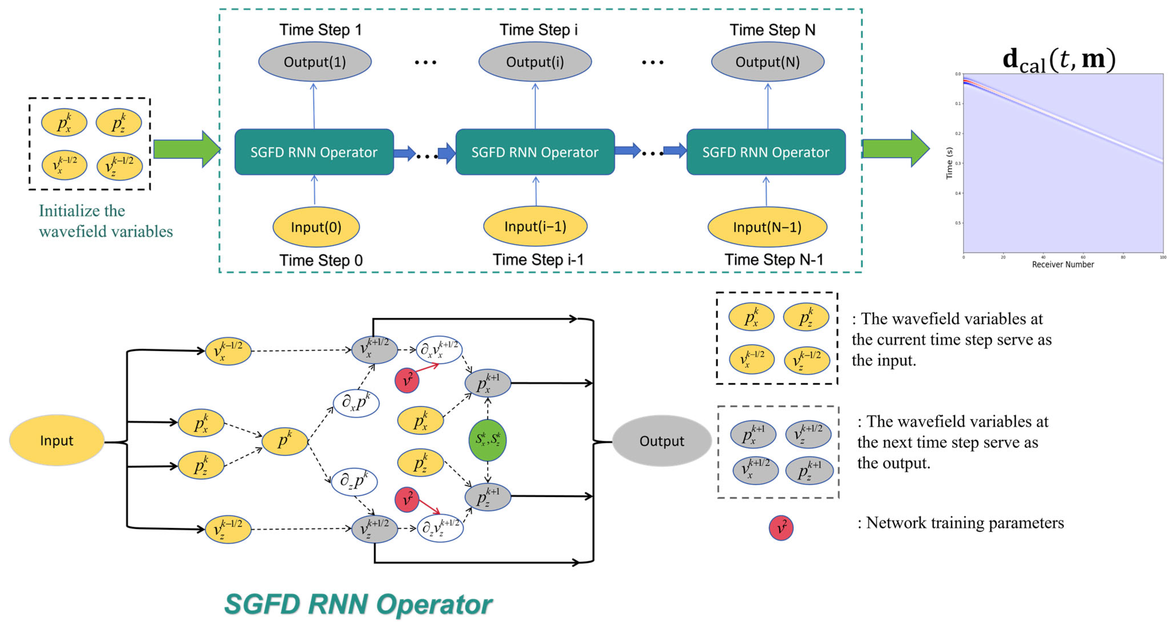
2.4.1. PIRNN Forward Modeling

We performed seismic forward modeling using the first-order pressure-velocity acoustic wave equation in homogeneous media, as shown in Equation (7):

$$\left\{\begin{array}{l}{\displaystyle \frac{\partial p_x(r,t)}{\partial t}}=v^2(r){\displaystyle \frac{\partial v_x(r,t)}{\partial x}}\hfill \\ {\displaystyle \frac{\partial p_z(r,t)}{\partial t}}=v^2(r){\displaystyle \frac{\partial v_z(r,t)}{\partial z}}\hfill \\ {\displaystyle \frac{\partial v_x(r,t)}{\partial t}}={\displaystyle \frac{\partial p(r,t)}{\partial x}}\hfill \\ {\displaystyle \frac{\partial v_z(r,t)}{\partial t}}={\displaystyle \frac{\partial p(r,t)}{\partial z}}\hfill \end{array}\right.,$$

(7)

where $p_x$ and $p_z$ are the pressure components in the x and z directions, respectively, $v_x$ and $v_z$ are the particle velocities in the x and z directions, respectively, and $r$ represents the spatial position of the wavefield variables; and $v\left(r\right)$ is the acoustic velocity to be inverted. When numerically solving wave equations, a time-stepping method is typically used, as it ensures that the wavefield state at each time step depends on the state of the previous time step. This characteristic aligns closely with the structure of RNNs, which can store information from previous time steps using hidden states [32]. These hidden states can be utilized to carry the wavefield information at each moment, connecting the gradient information across the entire spatiotemporal field. To further derive the time dependence of the wave equation, we discretized Equation (7) using finite differences on a second-order temporal accuracy staggered grid. Taking the $\mathrm{x}$-direction as an example [33]:

$$\left\{\begin{array}{l}{\displaystyle \frac{v_x^{k+\frac{1}{2}}[ix+\frac{1}{2},iz]-v_x^{k-\frac{1}{2}}[ix-\frac{1}{2},iz]}{\Delta t}}={\displaystyle \frac{p^k[ix+1,iz]-p^k[ix,iz]}{\Delta x}}\\ {\displaystyle \frac{p_x^{k+1}[ix,iz]-p_x^k[ix,iz]}{\Delta t}}=v^2[ix,iz]{\displaystyle \frac{v_x^{k+\frac{1}{2}}[ix+\frac{1}{2},iz]-v_x^{k+\frac{1}{2}}[ix-\frac{1}{2},iz]}{\Delta x}}\end{array}\right.,$$

(8)

Rearranging Equation (8) to obtain the recursive formulas for ${\mathrm{v}}_{\mathrm{x}}$ and $p_x$ produces:

$$\left\{\begin{array}{l}{v}_x^{k+{\displaystyle \frac{1}{2}}}[ix+{\displaystyle \frac{1}{2}},iz]={\displaystyle \frac{\Delta t[p^k[ix+1,iz]-p^k[ix,iz]]}{\Delta x}}+v_x^{k-{\displaystyle \frac{1}{2}}}[ix-{\displaystyle \frac{1}{2}},iz]\\ p_x^{k+1}[ix,iz]=v^2[ix,iz]\Delta t{\displaystyle \frac{v_x^{k+\frac{1}{2}}[ix+\frac{1}{2},iz]-v_x^{k+\frac{1}{2}}[ix-\frac{1}{2},iz]}{\Delta x}}+p_x^k[ix,iz]\end{array}\right.,$$

(9)

In each time iteration, the pressure ${\mathrm{p}}^{\mathrm{k}}$ at time $\mathrm{k}\Delta \mathrm{t}$ and particle velocity $v_x^{k-1/2}$ at time $\left(\mathrm{k}-1/2\right)\Delta t$ are first used to obtain the particle velocity $v_x^{k+1/2}$ at time $\left(\mathrm{k}+1/2\right)\Delta t$. Using the calculated particle velocity $v_x^{k+1/2}$ at $\left(\mathrm{k}+1/2\right)\Delta \mathrm{t}$ and pressure $p_x^k$ at $\mathrm{k}\Delta t$, the pressure $p_x^{k+1}$ is computed for the next time step. In this process, each time step of solving the wave equation utilizes wavefield data from the previous times $\mathrm{k}\Delta t$ and $\left(\mathrm{k}-1/2\right)\Delta t$. This temporal dependency enables seismic forward modeling using an RNN, where each layer of the RNN can be constructed to compute and store wavefield information at a specific time step. This structure can then be used to map the temporal evolution of the wavefield onto the hierarchical structure of the RNN. Specifically, each layer of the RNN represents the wavefield state at a particular time step, including the pressure and particle velocity. Within this framework, each RNN layer stores the current wavefield information and receives the output from the previous layer as the input. This architecture effectively simulates the temporal dependence of the wave equation, where the solution at each time step depends on the state of the previous time step. We integrated the PIRNN-based forward modeling process into an SGFD RNN Operator (Staggered Grid Finite Difference RNN Operator), with the complete forward modeling and loss calculation process shown in Figure 4. Here, $\mathrm{I}\mathrm{n}\mathrm{p}\mathrm{u}\mathrm{t}\left(i\right)$ represents the wavefield information stored in the RNN cell at time step $i$, while $\mathrm{O}\mathrm{u}\mathrm{t}\mathrm{p}\mathrm{u}\mathrm{t}\left(i\right)$ represents the simulated shot gather record ${\mathbf{d}}_{\mathrm{c}\mathrm{a}\mathrm{l}}\left(t_i,\mathbf{m}\right)$ generated at time step $i-1$. Starting with the initialized wavefield variables as input at time step 0, forward modeling is performed step by step through the SGFD RNN operator. During this process, velocity parameters are embedded into the RNN structure as trainable network parameters. Consequently, the resulting ${\mathbf{d}}_{\mathrm{c}\mathrm{a}\mathrm{l}}\left(t,\mathbf{m}\right)$ contains the chain relationships of the entire spatiotemporal field with respect to velocity parameters. This information enables the calculation of gradients of the current objective function with respect to velocity parameters during subsequent loss calculation and neural network backpropagation, thereby updating the velocity parameters.

2.4.2. PIRNN Full Waveform Inversion

The velocity model $\mathrm{v}$ is embedded as the trainable parameter within the PIRNN network architecture. The loss function is constructed based on the discrepancy between the observed and simulated data, utilizing the Mean Square Error (MSE) as the measurement metric:

$$J_{\mathrm{MSE}}(v)={\displaystyle \frac{1}{N_{s}T}}{\displaystyle \sum _{s=1}^{N_s}{\displaystyle \sum _{t=1}^T|}}|d_{\mathrm{cal}}(x_r,x_s,t,v)-d_{\mathrm{obs}}(x_r,x_s,t)|{|}^2,$$

(10)

where ${\mathrm{N}}_{\mathrm{s}}$ and $T$ represent the total number of time steps and ${\mathbf{d}}_{\mathrm{c}\mathrm{a}\mathrm{l}}$ and ${\mathbf{d}}_{\mathrm{o}\mathrm{b}\mathrm{s}}$ denote the simulated and observed data at the corresponding source locations and time steps, respectively. Within the PIRNN framework, the temporal dependencies between wavefield variables are transformed into chain relationships that were automatically recorded during the forward propagation process. The back-propagation algorithm computes the gradients of the loss function with respect to the model parameters. Because the velocity parameter $\mathrm{v}$ is embedded within the network, gradient information can be obtained through automatic differentiation mechanisms, and parameter updates can be performed using optimization algorithms, as shown in Equation (11):

$$v^{k+1}=v^k-\gamma {\displaystyle \frac{\partial J(v)}{\partial v}},$$

(11)

where $\mathsf{\gamma }$ is the learning rate. Sun [14] and Lu et al. [34] validated a PIRNN-based FWI method and demonstrated promising results. However, although this method reduces the dependency of FWI on the initial models, it can nonetheless lead to local minima when utilizing velocity models that lack prior knowledge and low-frequency information, resulting in inaccurate results. Therefore, this study introduces a first-arrival constrained physics-embedded recurrent neural network FWI method to ensure an FWI that is insensitive to initial velocity models.

3. Methodology

This section details the first arrival-constrained PIRNN full-waveform inversion method. This approach combines first-arrival wave information extraction, dynamic trace selection, and progressive strategies to minimize the dependency on initial velocity models and ensure stable inversion results.

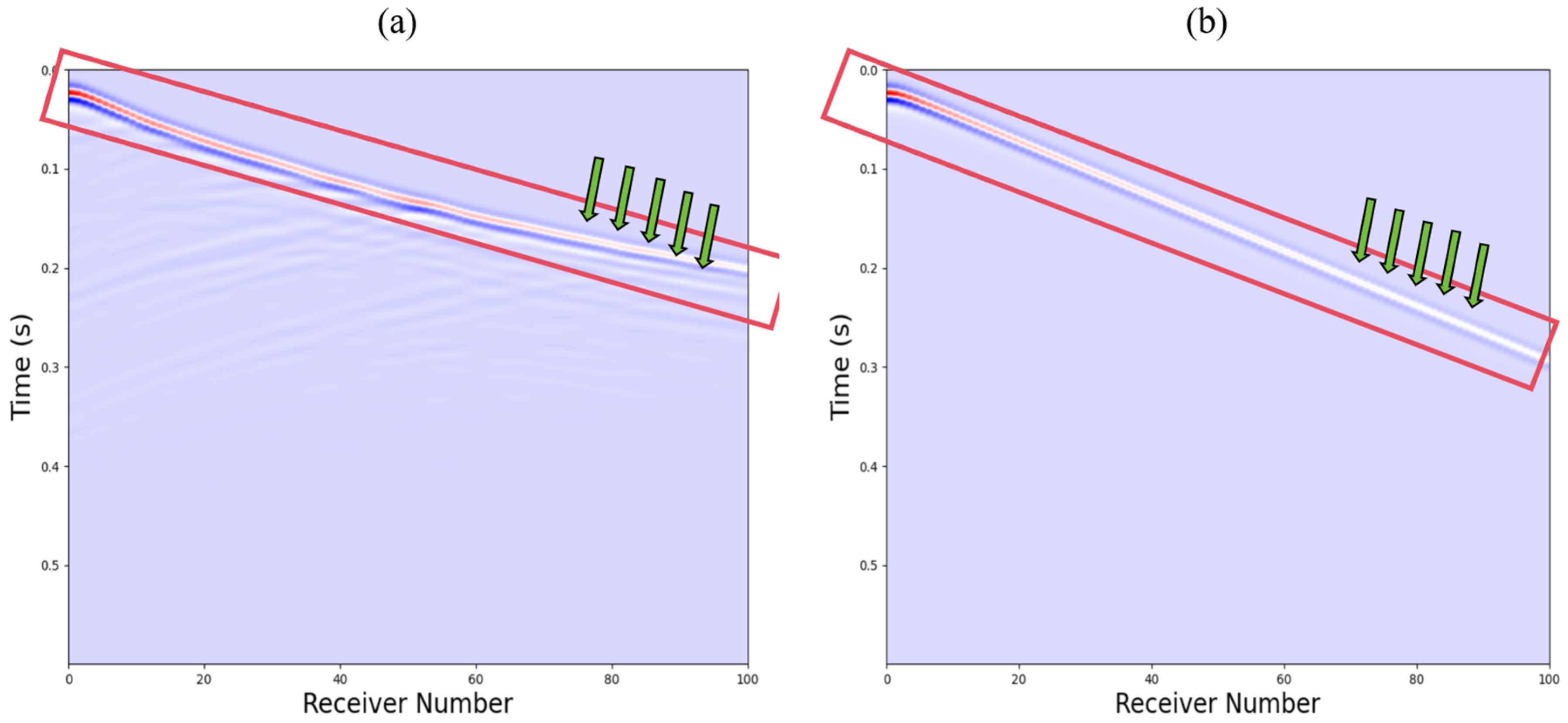
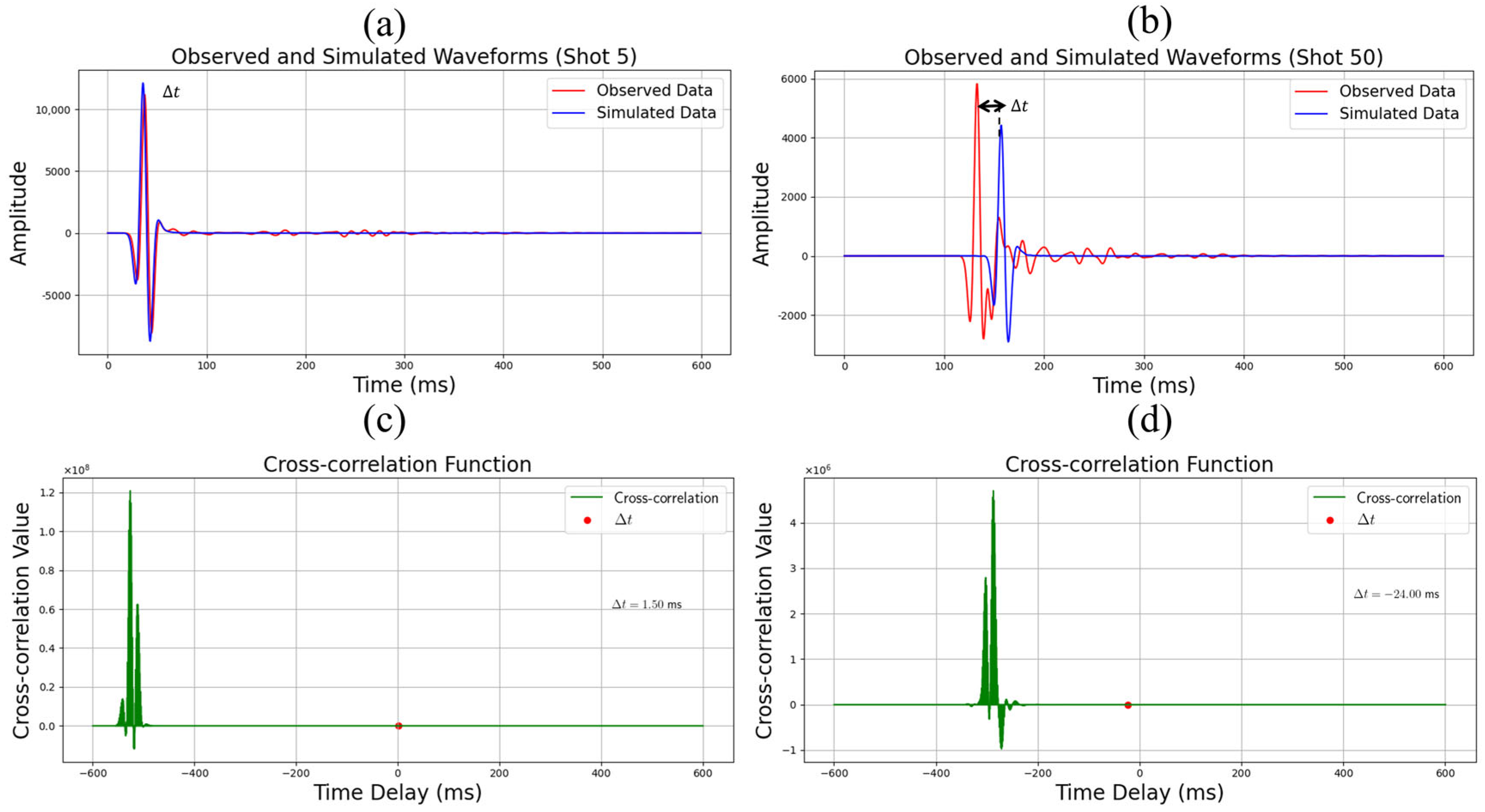
3.1. Extraction Method of First-Arrival Information

In VSP, first-arrival waves, which are the earliest wave motions that reach receivers, are an important component in FWIs. First arrivals typically represent the initial wave propagations along the shortest paths through subsurface media, and their arrival times and propagation characteristics provide crucial information about velocity structures. An effective extraction and utilization of first-arrival information can significantly enhance the stability and accuracy of full-waveform inversion. In the present study, we extracted first-arrival time differences by computing cross-correlation functions between the observed and simulated data and used these differences to select appropriate seismic traces for inversion.

Consider a single seismic trace, where ${\mathbf{d}}_{\mathrm{o}\mathrm{b}\mathrm{s}}^{\mathrm{s}}\left(t\right)$ and ${\mathbf{d}}_{\mathrm{c}\mathrm{a}\mathrm{l}}^{\mathrm{s}}\left(t\right)$ represent the observed and simulated data, $\mathrm{s}$ denotes the trace index, and $\mathrm{t}$ denotes time. Each trace consists of a time series. To extract the temporal difference in first arrivals between observed and simulated data, we computed their cross-correlation function ${\mathcal{C}}^s\left(\tau \right)$ as follows:

$${\mathcal{C}}^s(\tau )={\displaystyle \int d_{\mathrm{obs}}^s}(t)d_{\mathrm{cal}}^s(t+\tau )dt,$$

(12)

where $\tau$ denotes the time lag. We designated the peak position ${\tau }_{max}^s$ the cross-correlation function as the optimal temporal alignment between the observed and synthetic data for this trace, expressed as follows:

$${\tau }_{\max }^s=\arg {\max }_{\tau }{\mathcal{C}}^s(\tau ),$$

(13)

The peak position ${\tau }_{max}^s$ indicates the temporal discrepancy in first-arrival times between simulated and observed data. The magnitude of $\left|{\tau }_{\mathrm{m}\mathrm{a}\mathrm{x}}^{\mathrm{s}}\right|$ increases proportionally with the disparity between the initial velocity model and the true model. Including traces with substantial discrepancies in loss computation and gradient, backpropagation can potentially lead to erroneous parameter update directions. To quantify this temporal discrepancy, we defined a metric by subtracting the total finite difference simulation time $\mathrm{T}$ from ${\mathsf{\tau }}_{\mathrm{m}\mathrm{a}\mathrm{x}}^{\mathrm{s}}$, yielding the following:

$$\Delta t^s={\tau }_{\max }^s-T,$$

(14)

where $\Delta t^{\mathrm{s}}$ denotes the temporal phase differential between the observed and simulated data for the $\mathrm{s}$-th seismic trace. This first-arrival phase differential serves as the criterion for dynamic trace selection in the loss computation. We established a temporal threshold $\Delta t_{\mathrm{t}\mathrm{h}\mathrm{r}\mathrm{e}\mathrm{s}\mathrm{h}\mathrm{o}\mathrm{l}\mathrm{d}}$, where traces satisfying $\left|\Delta t^s\right|<\Delta t_{\mathrm{t}\mathrm{h}\mathrm{r}\mathrm{e}\mathrm{s}\mathrm{h}\mathrm{o}\mathrm{l}\mathrm{d}}$ exhibited sufficient coherence between their embedded subsurface velocity information and the current initial model; conversely, traces exceeding this threshold were temporarily omitted from the loss computation. The mathematical formulation is as follows:

$${𝒮}_{\mathrm{selected}}=\left\{s\in 𝒮| |\Delta t^s|<\Delta t_{\mathrm{threshold}}\right\},$$

(15)

where $𝒮$ denotes the complete ensemble of seismic traces and ${𝒮}_{\mathrm{selected}}$ represents the subset of selected traces. This dynamic selection mechanism ensures that during the initial stages of inversion, when the disparity between the initial and true models is substantial, the inversion process exclusively incorporates traces that exhibit minimal first-arrival phase differentials between the observed and synthetic data. This methodology effectively mitigates the propagation of errors stemming from initial velocity model inaccuracies and enhances the inversion stability. As the inversion evolves, additional seismic traces are progressively incorporated into the inversion process. This methodological approach initiates inversion with high-fidelity data and systematically expands the dataset, thereby circumventing local minima that can arise from data insufficiency and optimizing the comprehensiveness of the inversion results.

3.2. FWI Objective Function with First-Arrival Constraints

The conventional full waveform inversion (FWI) objective function (Equation (10)) quantifies the data misfit between the observed and synthetic seismic traces across all receivers. However, this formulation may result in inversion instability owing to initial model dependencies. To mitigate this limitation, we introduced a dynamic objective function that incorporates first-arrival constraints:

$$J(v)={\displaystyle \sum _{s\in {𝒮}_{\mathrm{selected}}}{\displaystyle \sum _{t=1}^T\Vert d_{\mathrm{cal}}^s(}}t;v)-d_{\mathrm{obs}}^s(t){\Vert }^2,$$

(16)

where ${\mathbf{d}}_{\mathrm{c}\mathrm{a}\mathrm{l}}^s\left(\mathrm{t};\mathbf{v}\right)$ denotes the synthetic seismogram at time step $\mathrm{t}$ for the s-th trace, ${\mathbf{d}}_{\mathrm{o}\mathrm{b}\mathrm{s}}^s\left(\mathrm{t}\right)$ represents the corresponding observed seismogram, and $\mathrm{T}$ denotes the total number of temporal samples. This loss function exclusively incorporates seismic traces from the subset ${𝒮}_{\mathrm{selected}}$, thereby amplifying the contribution of the first-arrival phase matching and attenuating the influence of the initial model uncertainties.

3.3. Network Structure

The network structure is shown in Figure 5. During each iteration, we forward-propagated the initial model through the SGFD RNN operator to generate synthetic data and recorded the gradient information of the entire space-time field. We then filtered the seismic traces based on the first arrival constraints by comparing the synthetic data with the observed data. The selected traces were used to calculate the loss, which was then backpropagated to update the initial model. This process was repeated until most traces were selected for computation, the total first arrival time difference approached zero, and the loss function converged to a preset threshold.

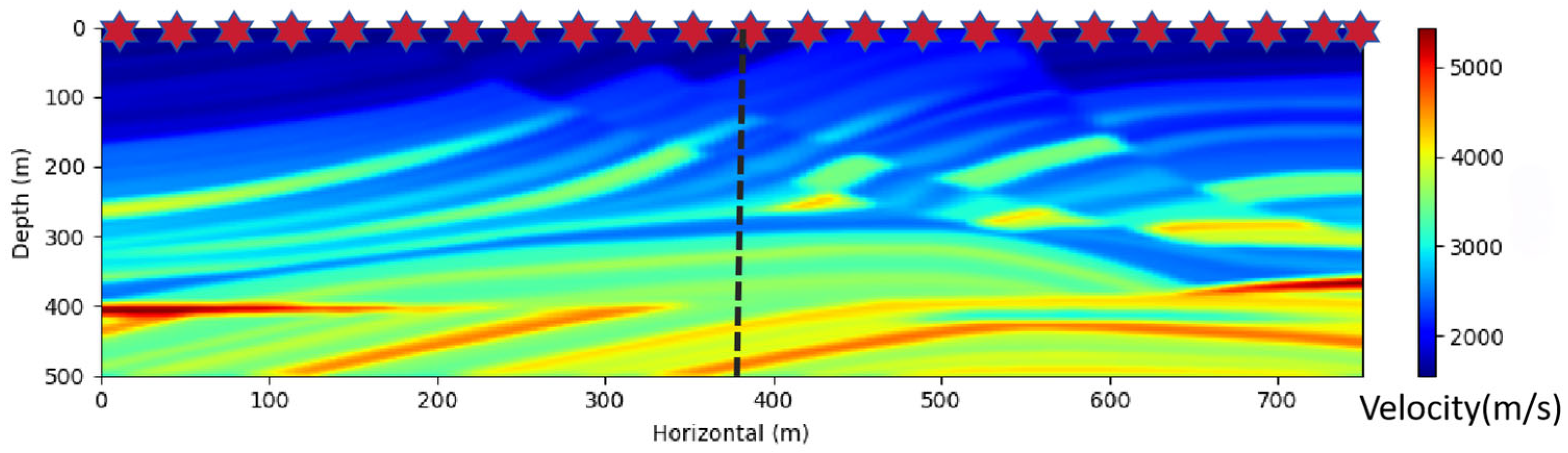
4. Numerical Application

We conducted numerical experiments to evaluate the effectiveness and robustness of the proposed method in mitigating the dependency on the initial models. We selected two velocity models: the 2D acoustic Marmousi model and the 2007 BP TTI anisotropic velocity benchmark model. For the first test, the model grid size was 100 × 150 with a grid spacing of 5 m. In the forward modeling process, we employed a Ricker wavelet with a dominant frequency of 50 Hz as the source and applied a free surface and perfectly matched layer (PML) absorbing boundary conditions at the top and other boundaries, respectively. We uniformly deployed 85 sources along the surface with a source spacing of 8–10 m and utilized a VSP observation system for data acquisition. In addition, the 2007 BP TTI anisotropic velocity benchmark model was employed as a test case. This model, created by Hemang Shah and provided by the BP Exploration Operation Company Limited, is a two-dimensional anisotropic velocity model. In this study, only the P-wave velocity (${\mathrm{v}}_{\mathrm{p}}$) component of the model was used to test the performance of the inversion algorithm in complex media. Figure 6 shows the velocity distribution and observation system setup for the Marmousi model and Figure 7 displays the ${\mathrm{v}}_{\mathrm{p}}$ velocity distribution and observation system setup for the 2007 BP model. All numerical simulations and inversions were performed using identical computational resources, primarily NVIDIA A800 GPUs on a Linux system with a PyTorch (version 2.4.1) deep-learning framework.

4.1. Evaluation Metrics

4.1.1. Coefficient of Determination ($R^2$ Score)

The ${\mathrm{R}}^2$ score was used to measure the linear correlation between the inversion results and the true model, which is defined as follows:

$$R^2=1-{\displaystyle \frac{{\displaystyle \sum _{i=1}^N{(v_i^{inv}-v_i^{true})}^2}}{{\displaystyle \sum _{i=1}^N{(v_i^{true}-{\overline{v}}^{true})}^2}}}$$

(17)

where ${\mathrm{v}}_{\mathrm{i}}^{\mathrm{i}\mathrm{n}\mathrm{v}}$ represents the velocity value of the ith grid point obtained from the inversion, ${\mathrm{v}}_{\mathrm{i}}^{\mathrm{t}\mathrm{r}\mathrm{u}\mathrm{e}}$ represents the velocity value of the ith grid point in the true model, ${\overline{\mathrm{v}}}^{\mathrm{t}\mathrm{r}\mathrm{u}\mathrm{e}}$ represents the average velocity value of the true model, and $\mathrm{N}$ represents the total number of grid points. The range of an ${\mathrm{R}}^2$ score is $\left(-\mathrm{\infty },1\right]$, where values closer to 1 indicate a stronger linear correlation between the inversion results and the true model, and vice versa.

4.1.2. Structural Similarity Index Measure (SSIM)

The SSIM was used to evaluate the structural similarity between the inversion results and the true model, which is defined as follows:

$$SSIM(x,y)={\displaystyle \frac{(2{\mu }_x{\mu }_y+c_1)(2{\sigma }_{xy}+c_2)}{({\mu }_x^2+{\mu }_y^2+c_1)({\sigma }_x^2+{\sigma }_y^2+c_2)}}$$

(18)

where $\mathrm{x}$ and $\mathrm{y}$ represent the velocity values of the inversion results and true model within a local window, respectively, ${\mu }_x$ and ${\mu }_y$ represent the mean values of $x$ and $y$, respectively, ${\mathsf{\sigma }}_{\mathrm{x}}$ and ${\mathsf{\sigma }}_{\mathrm{y}}$ represent the standard deviations of $x$ and $y$, respectively, ${\mathsf{\sigma }}_{\mathrm{x}\mathrm{y}}$ represents the covariance between $x$ and $y$, and ${\mathrm{c}}_1$ and ${\mathrm{c}}_2$ are constants introduced to avoid zero denominators. The range of SSIM is [0, 1], where values closer to 1 indicate a higher structural similarity between the inversion results and the true model, and vice versa.

4.1.3. Normalized Cross-Correlation (NCC)

NCC is used to measure the overall similarity between the inversion results and the true model and is defined as follows:

$$NCC(x,y)={\displaystyle \frac{{\displaystyle \sum _{i=1}^N(x_i-\overline{x})}(y_i-\overline{y})}{\sqrt{{\displaystyle \sum _{i=1}^N{(x_i-\overline{x})}^2}}\sqrt{{\displaystyle \sum _{i=1}^N{(y_i-\overline{y})}^2}}}}$$

(19)

where ${\mathrm{x}}_{\mathrm{i}}$ and $y_i$ represent the velocity values at the $\mathrm{i}$-th grid point of the inversion results and the true model, respectively, $\overline{x}$ and $\overline{y}$ represent the average velocity values of the inversion results and the true model, respectively, and $N$ represents the total number of grid points. The range of the NCC is [−1, 1], where values closer to 1 indicate a higher overall similarity between the inversion results and true model, values closer to −1 indicate a negative correlation between the inversion results and true model, and values closer to 0 indicate no correlation between the inversion results and true model.

4.2. Initial Model Dependency

We next evaluated the effectiveness of our proposed Physics-Informed Recurrent Neural Network with First-Arrival Constraints for Full Waveform Inversion (PIRNN-FAC-FWI, abbreviated as FAFWI) method in mitigating the initial model dependency through a comparative analysis using the Marmousi model. As a nonlinear optimization problem, FWI results are highly sensitive to the quality of the initial velocity model. When there are significant differences between the initial and true models, FWI tends to fall into local minima, leading to inaccurate inversion results. To verify that our proposed FAFWI method can effectively reduce the dependency on the initial models, we used a constant-velocity model as the initial model for full waveform inversion. This initial model differs significantly from the true velocity model, which lacks both low-frequency and well-log information and thus presents a challenging initial model for FWI. Furthermore, to ensure experimental consistency, the Adam optimization algorithm was used for the various FWI methods, with the time threshold $\Delta {\mathrm{t}}_{\mathrm{threshold}}$ set to 2.5 ms, and the learning rate was uniformly set to 40 and kept constant. Numerical experiments were conducted using a 2D acoustic Marmousi model.

4.3. Robustness Analysis

To evaluate the robustness of the proposed FAFWI method comprehensively, this section presents analyses from three aspects: method applicability, noise impact, and initial model sensitivity. First, we verified the applicability of the method in complex media by testing it on velocity models of varying complexities, specifically, the 2007 BP TTI model. Second, we assessed the stability and noise resistance of the method by introducing noise interference. Finally, we analyzed the sensitivity of the method to the initial models by testing different initial velocity models. Through these experiments, we aimed to thoroughly evaluate the reliability and adaptability of the FAFWI method for practical applications.

4.3.1. Method Applicability

To evaluate the applicability of the FAFWI method to complex media, the 2007 BP TTI P-wave velocity model was selected as the test case. The initial velocity model was set as a homogeneous medium with a uniform velocity of 1900 m/s at all the grid points.

4.3.2. Noise Analysis

In a practical seismic data inversion, noise is an inevitable interference factor; thus, evaluating the robustness of the FAFWI method under various noise conditions is important. We incorporated Gaussian white noise with a standard deviation of $\sigma =2{\sigma }_0$ into the noise-free observational data of the Marmousi model, where ${\sigma }_0$ denotes the standard deviation of the noise-free data.

4.3.3. Initial Model Sensitivity Analysis

The Marmousi model was used to test the sensitivity of the FAFWI method to different initial models. In the validation, we used a constant velocity model of 1800 m/s as the initial model. We then gradually increased this velocity value to test constant velocity models of 2100, 2300, and 2500 m/s as the initial models. These values represent the average velocities from the shallow to deeper regions around the well.

5. Results

5.1. Initial Model Dependency

Figure 8a shows the initial constant-velocity model used in the Marmousi inversion, where the velocity at each point was 1800 m/s. Without incorporating any prior structural information as a constraint, this velocity model easily falls into local minima under conventional FWI, resulting in incorrect physical solutions. The corresponding true Marmousi velocity model is presented in Figure 8b. The inversion results under conventional FWI exhibited high uncertainty and deviated completely from the true velocity structure (Figure 8c). The inversion results obtained using our proposed method were compared against the conventional FWI (Figure 8d). Under the same initial model, the FAFWI method produced relatively accurate inversion results within the effective range of the VSP observation system. FAFWI reconstructed the velocity structures in the shallow and middle layers and successfully inverted the velocity structure and variation trends in deep regions. To quantitatively evaluate the velocity field characteristics in the vicinity of the wellbore, vertical velocity profiles at distances of ±75 m from the wellbore center were extracted (Figure 9). The profile comparison analysis indicated that the inversion results showed high consistency with the true model in most regions, from the shallow to deep layers.

The effective inversion area exhibited a distinct inverted triangular pattern based on the spatial distribution characteristics of the velocity field inversion results. This result is consistent with the physical principles; as in the VSP observation system, the geophones are arranged vertically along the wellbore, making it difficult to effectively receive seismic reflections from lateral areas far from the shot-well pairs. Based on this difficulty, we calculated the ${\mathrm{R}}^2$ score, Structural Similarity Index (SSIM), and the normalized correlation coefficient between the inversion results and true model within this range to comprehensively evaluate the linear correlation and structural similarity of the results obtained by the FAFWI method when starting from the 1800 m/s constant-velocity initial model shown in Figure 8a for the Marmousi case. The results are summarized in

Table 1. Quantitative comparison of inversion results using the FAFWI method on the Marmousi model.

Parameters	Marmousi
${\mathrm{R}}^2$ Score	0.5471
SSIM	0.8390
Correlation Coefficient	0.7858

. The model inverted by our proposed FAFWI method demonstrated a strong linear relationship and structural similarity with the true model (Table 1) as well as advantages in terms of the normalized correlation.

As the inversion process continues, the velocity parameters are updated in the correct direction, leading to an increasing number of seismic traces satisfying $\left|\Delta {\mathrm{t}}^{\mathrm{s}}\right|<\Delta {\mathrm{t}}_{\mathrm{t}\mathrm{h}\mathrm{r}\mathrm{e}\mathrm{s}\mathrm{h}\mathrm{o}\mathrm{l}\mathrm{d}}$ in Equation (15) in each iteration. The total phase difference $\mathsf{\tau }={\sum }_{\mathrm{s}=1}^{\mathrm{s}\mathrm{h}\mathrm{o}\mathrm{t}\mathrm{s}}\Delta {\mathrm{t}}^{\mathrm{s}}$ gradually approaches 0, and the number of selected seismic traces shows an upward trend. These phenomena are reflected in the training metrics of the Marmousi model (Figure 10). This dynamic adjustment mechanism implements the dynamic objective function in Equation (16). As the inversion progresses, more seismic traces are included, resulting in more comprehensive and accurate inversion results.

5.2. Robustness Analysis

5.2.1. Method Applicability

The true velocity model (Figure 11a) exhibited more complex structural features than the initial velocity model. Specifically, there is a significant high-velocity anomaly in the left region of the model located outside the effective inversion area of the vertical seismic profile (VSP), which poses a challenge to the inversion process. Additionally, another high-velocity anomaly exists near the wellbore, where the vertical velocity gradient is large, forming significant velocity discontinuities that further increase the inversion difficulty. Figure 11b shows the inversion results obtained by FAFWI, demonstrating that the method accurately reconstructed the velocity structure from shallow to deep depths and precisely recovered the location and structure of both high-velocity anomalies. Similarly, we extracted velocity profiles at 75 m left and 100 m right of the wellbore (Figure 12). At a depth of 90 m, the velocity value abruptly jumped from 1700 to 4300 m/s and then transitioned back to 2300 m/s at a depth of 150 m (Figure 12a). Despite these significant velocity discontinuities, the FAFWI method accurately inverted the structural information of velocity variations. For regions with more gradual velocity structures (Figure 11b), the FAFWI inversion results almost perfectly matched the true model, indicating a high inversion accuracy. The R² score, structural similarity index (SSIM), and normalized correlation coefficient were calculated for the inversion results within this range and were compared with the true model (

Table 2. Quantitative comparison of inversion results using the FAFWI method for the BP TTI model.

Parameters	BP TTI
${\mathrm{R}}^2$ Score	0.9118
SSIM	0.8413
Correlation Coefficient	0.9566

). The results are similar to those of previous studies; the inverted model showed strong linear relationships and structural similarity with the true model. The results demonstrated that the FAFWI method is applicable to different velocity models and is not limited to specific velocity structures.

5.2.2. Noise Analysis

Figure 13 illustrates the VSP shot gathers for both far and near offsets after noise addition, with the left panel showing the noise-free shot gather and the right panel displaying the shot gather with a $2{\mathsf{\sigma }}_0$ noise level. In the experimental implementation, the FAFWI method was initialized using the constant-velocity model (Figure 8a), and the inversion was performed using noise-contaminated observational data.

Figure 14 shows the inversion results of the FAFWI method for the Marmousi model under noisy conditions. Specifically, (a) presents the inversion result under noise-free conditions, (b) illustrates the inversion result under the $2{\mathsf{\sigma }}_0$ noise level. The FAFWI method maintained a high inversion accuracy even under $2{\mathsf{\sigma }}_0$ noise conditions through successfully reconstructing the velocity structures in both shallow and middle layers. However, the coverage area in the inverted-triangular region showed a reduction, which may be attributed to the loss of high-frequency information owing to noise interference. Nevertheless, the resolution and accuracy of the inversion results were sufficient to meet the imaging requirements. Overall, the FAFWI method demonstrated considerable noise robustness and maintained a high inversion accuracy despite noise interference.

5.2.3. Initial Model Sensitivity Analysis

The initial models are shown in Figure 15. Figure 16 shows the inversion results of the FAFWI method with different initial constant-velocity models. In (a), with an initial model speed of 1800 m/s, the FAFWI method successfully reconstructed the velocity structures in both the shallow and middle layers, showing a high trend consistency in the deep regions. In (b), with a velocity of 2100 m/s, the overall velocity structure remains clear but shows slightly less consistency than (a). When the initial velocity increased to 2300 m/s, as shown in (c), there was a noticeable increase in the regions trapped in the local minima. Finally, when the initial velocity reached 2500 m/s, approaching the average velocity of the middle layer, large areas of the inversion results became trapped in local minima, leading to a decreased inversion accuracy. The experimental results indicate that the inversion is more accurate when the initial constant-velocity model is closer to the average velocity of the shallow layers near the well. Conversely, higher initial velocities are more likely to result in local minimum traps. Overall, although the FAFWI method demonstrated some insensitivity to the initial models, inversion results may fail because of local minima when the initial model velocities are excessively high.

6. Discussion

6.1. Analysis

Our numerical experiments demonstrated the effectiveness and robustness of the proposed FAFWI method. By utilizing the first-arrival time information and dynamically selecting seismic traces with minimum phase differences, the FAFWI-PIRNN effectively reduced the dependence on the initial velocity models. A comparison of the inversion results with conventional FWI methods in the Marmousi and 2007 BP TTI velocity models demonstrated the capability of the proposed method to navigate complex subsurface structures and avoid the local minimum traps faced by traditional FWI.

FAFWI demonstrated dual utilization of first-arrival and reflection wave information. Unlike traditional first-arrival FWI methods, which rely solely on the earliest arriving waves, our method integrates reflection wave information through a first-arrival difference selection mechanism. This integration improves the fidelity of velocity model reconstruction and ensures more comprehensive seismic information utilization, thereby enhancing the overall resolution and accuracy of the inversion results. The dynamic selection of seismic traces based on first-arrival delays ensured that only traces with reliable first-arrival and reflection wave information participated in the inversion process, thereby improving the stability and robustness of the method. Furthermore, we enhanced the FAFWI performance by incorporating a Physics-Informed Recurrent Neural Network (PIRNN). The PIRNN framework embeds physical wave propagation processes into the recurrent neural network, facilitates the integration of physical constraints during network training, and fully utilizes the spatiotemporal field gradients recorded during forward propagation for back propagation, providing nonlinear solutions for full-waveform inversion and ensuring that the results conform to geophysical principles. We comprehensively evaluated the performance of the method based on four aspects: effectiveness, applicability, noise resistance, and initial model sensitivity.

When compared with other strategies aimed at reducing initial model dependency or similar issues, the FAFWI-PIRNN method presents several key distinctions. Multiscale FWI [4], optimal transport [9], and adaptive waveform inversion [7] primarily focus on reshaping the optimization problem or the data itself to be less prone to cycle-skipping. In contrast, the FAFWI-PIRNN method dynamically selects seismic traces based on first-arrival constraints and inputs the full information of these traces into a physically consistent PIRNN. This differs from solely using traveltime tomography to build an initial model [29]. In the realm of deep learning, unlike data-driven FWI methods [13,14], our approach maintains strong physical constraints via the PIRNN while leveraging first-arrival information for data selection, rather than relying predominantly on learning from large datasets or network-induced regularization

6.2. First-Arrival Time Picking Methods

In this study, the first-arrival phase-difference picking method relied on cross-correlation calculations. However, under high-noise conditions, the cross-correlation results can interfere, leading to inaccurate first-arrival time picking. In such cases, incorrect seismic trace selection may introduce misleading velocity updates, thereby affecting the accuracy of inversion results. Therefore, future research should explore more precise first-arrival time extraction methods combined with noise suppression techniques to enhance the reliability of the first-arrival information extraction.

7. Conclusions

This study presents a novel Physics-Informed Recurrent Neural Network Full Waveform Inversion method with first-arrival constraints (PIRNN-FAFWI) to reduce the sensitivity of FWI to initial velocity models. Our method utilized the information contained in first-arrival waveforms to select seismic traces dynamically for loss calculations and effectively reduced the impact of inaccurate initial models on the inversion process. This dynamic selection, combined with a progressive strategy that gradually introduced more seismic traces as the inversion progressed, ensured a stable and robust inversion workflow. Our method integrated both first-arrival and reflected wave data, by computing the cross-correlation between the observed and simulated data, we extracted the first arrival time differences and used them to select appropriate seismic traces for inversion, thereby improving the robustness and resolution of the results. Through numerical experiments using the 2D acoustic Marmousi model and 2007 BP TTI anisotropic velocity benchmark model, we demonstrated the effectiveness and robustness of this method in reducing the dependence on initial velocity models. The FAFWI method inverted accurate velocity models, even with poor initial models. Quantitative analyses using metrics such as ${\mathrm{R}}^2$, SSIM, and NCC further confirmed the excellent performance of the proposed method in terms of linear correlation, structural similarity, and overall similarity with the true velocity model. In future studies, we will employ more precise first-arrival picking methods and investigate noise suppression techniques to further enhance the FAFWI performance.

In future studies, we will employ more precise first-arrival picking methods and investigate noise suppression techniques to further enhance the FAFWI-PIRNN performance. Furthermore, to more comprehensively assess the robustness and generalization capabilities of the proposed method, future work could explore its performance under a wider and more diverse range of initial velocity models, encompassing varying structural complexities, noise levels, and degrees of deviation from the true model. Additionally, although the first-arrival constraints in FAFWI-PIRNN effectively address cycle-skipping related local minima, further investigation into the optimization process itself, such as the impact of different optimizers, learning rate schedules, and regularization techniques on potential oscillations or suboptimal local minima encountered during the inversion, could lead to further improvements in solution quality and convergence reliability.

References

1. Tarantola, A. Inversion of seismic reflection data in the acoustic approximation. Geophysics 1984, 49, 1259–1266. [Google Scholar] [CrossRef]
2. Tarantola, A. Linearized inversion of seismic reflection data. Geophys. Prospect. 1984, 32, 998–1015. [Google Scholar] [CrossRef]
3. Virieux, J.; Operto, S. An overview of full-waveform inversion in exploration geophysics. Geophysics 2009, 74, WCC1–WCC26. [Google Scholar] [CrossRef]
4. Fang, Z.; Grobbe, N.; Slob, E.; Wapenaar, K. Source estimation for wavefield-reconstruction inversion. Geophysics 2018, 83, R345–R359. [Google Scholar] [CrossRef]
5. Biondi, B.; Almomin, A. Simultaneous inversion of full data bandwidth by tomographic full-waveform inversion. Geophysics 2014, 79, WA129–WA140. [Google Scholar] [CrossRef]
6. Bunks, C.; Saleck, F.M.; Zaleski, S.; Chavent, G. Multiscale seismic waveform inversion. Geophysics 1995, 60, 1457–1473. [Google Scholar] [CrossRef]
7. van Leeuwen, T.; Herrmann, F.J. Mitigating local minima in full-waveform inversion by expanding the search space. Geophys. J. Int. 2013, 195, 661–667. [Google Scholar] [CrossRef]
8. Esser, E.; Guasch, L.; van Leeuwen, T.; Aravkin, A.; Herrmann, F.J. Total-variation regularization strategies in full-waveform inversion. SIAM J. Imaging Sci. 2018, 11, 376–406. [Google Scholar] [CrossRef]
9. Warner, M.; Guasch, L. Adaptive waveform inversion: Theory. Geophysics 2016, 81, R429–R445. [Google Scholar] [CrossRef]
10. Yang, Y.; Engquist, B. Analysis of optimal transport and related misfit functions in full-waveform inversion. Geophysics 2018, 83, A7–A12. [Google Scholar] [CrossRef]
11. Yang, Y.; Engquist, B.; Sun, J.; Hamfeldt, B.F. Application of optimal transport and the quadratic Wasserstein metric to full-waveform inversion. Geophysics 2018, 83, R43–R62. [Google Scholar] [CrossRef]
12. Chi, B.; Dong, L.; Liu, Y. Full waveform inversion method using envelope objective function without low frequency data. J. Appl. Geophys. 2014, 109, 36–46. [Google Scholar] [CrossRef]
13. Oh, J.-W.; Alkhalifah, T. Full waveform inversion using envelope-based global correlation norm. Geophys. J. Int. 2018, 213, 815–823. [Google Scholar] [CrossRef]
14. Sun, J.; Li, J.; Zhang, J.; Chen, X. A theory-guided deep-learning formulation and optimization of seismic waveform inversion. Geophysics 2020, 85, R87–R99. [Google Scholar] [CrossRef]
15. Zhang, Z.; Lin, Y. Data-driven seismic waveform inversion: A study on the robustness and generalization. IEEE Trans. Geosci. Remote Sens. 2020, 58, 6900–6913. [Google Scholar] [CrossRef]
16. Wu, Y.; Lin, Y. InversionNet: An efficient and accurate data-driven full waveform inversion. IEEE Trans. Comput. Imaging 2019, 6, 419–433. [Google Scholar] [CrossRef]
17. Raissi, M.; Perdikaris, P.; Karniadakis, G.E. Physics-informed neural networks: A deep learning framework for solving forward and inverse problems involving nonlinear partial differential equations. J. Comput. Phys. 2019, 378, 686–707. [Google Scholar] [CrossRef]
18. Rasht-Behesht, M.; Gholami, A.; Kamal, M.; Siahkoohi, H.R. Physics-informed neural networks (PINNs) for wave propagation and full waveform inversions. J. Geophys. Res. Solid Earth 2022, 127, e2021JB023120. [Google Scholar] [CrossRef]
19. Sun, J.; Niu, Z.; Innanen, K.A.; Li, J.; Trad, D.O. Physics-guided deep learning for seismic inversion with hybrid training and uncertainty analysis. Geophysics 2021, 86, R303–R317. [Google Scholar] [CrossRef]
20. Du, B.; Liu, Y.; Wang, Y. Physics-informed robust and implicit full waveform inversion without prior and low-frequency information. IEEE Trans. Geosci. Remote Sens. 2024, 62, 5918712. [Google Scholar] [CrossRef]
21. Zhu, W.; Geng, Y.; Dickson, A.D.; Lin, Y. Integrating deep neural networks with full-waveform inversion: Reparameterization, regularization, and uncertainty quantification. Geophysics 2022, 87, R93–R109. [Google Scholar] [CrossRef]
22. Zhou, L.; Chen, S.; Song, H.; Liu, Y.; Zhang, H. Full waveform inversion based on dynamic data matching of convolutional wavefields. Front. Earth Sci. 2023, 11, 1134871. [Google Scholar] [CrossRef]
23. Zhang, J.; Chen, J. Joint seismic traveltime and waveform inversion for near surface imaging. In Proceedings of the SEG International Exposition and Annual Meeting, Denver, CO, USA, 26–31 October 2014; Society of Exploration Geophysicists: Tulsa, OK, USA, 2014; p. SEG-2014-1501. [Google Scholar]
24. Treister, E.; Haber, E. Joint full waveform inversion and travel time tomography. In Proceedings of the 78th EAGE Conference and Exhibition 2016, Vienna, Austria, 30 May–2 June 2016; European Association of Geoscientists & Engineers: Houten, The Netherlands, 2016; pp. 1–5. [Google Scholar]
25. Tsai, K.C.; Wu, Y.H.; Lin, T.Y. First-break automatic picking with deep semisupervised learning neural network. In SEG Technical Program Expanded Abstracts 2018; Society of Exploration Geophysicists: Tulsa, OK, USA, 2018; pp. 2181–2185. [Google Scholar]
26. Wang, H.; Chen, Y.; Ma, J. Seismic first break picking in a higher dimension using deep graph learning. arXiv 2024, arXiv:2404.08408. [Google Scholar]
27. Wen, Z.; Ma, J. Effective First-Break Picking of Seismic Data Using Geometric Learning Methods. Remote Sens. 2025, 17, 232. [Google Scholar] [CrossRef]
28. Stewart, R.R.; Huddleston, P.D.; Kan, T.K. Seismic versus sonic velocities: A vertical seismic profiling study. Geophysics 1984, 49, 1153–1168. [Google Scholar] [CrossRef]
29. Yilmaz, O. Seismic Data Analysis: Processing, Inversion and Interpretation of Seismic Data; Society of Exploration Geophysicists: Tulsa, OK, USA, 2001. [Google Scholar]
30. Sheriff, R.E.; Geldart, L.P. Exploration Seismology; Cambridge University Press: Cambridge, UK, 1995. [Google Scholar] [CrossRef]
31. Sirgue, L.; Pratt, R.G. Efficient waveform inversion and imaging: A strategy for selecting temporal frequencies. Geophysics 2004, 69, 231–248. [Google Scholar] [CrossRef]
32. Goodfellow, I.; Bengio, Y.; Courville, A. Deep Learning; MIT Press: Cambridge, MA, USA, 2016. [Google Scholar]
33. Yang, P. A Numerical Tour of Wave Propagation; Xi’an Jiaotong University Press: Xi’an, China, 2014. [Google Scholar]
34. Lu, C.; Liu, J.; Qu, L.; Gao, J.; Cai, H.; Liang, J. Elastic full-waveform inversion via physics-informed recurrent neural network. IEEE Trans. Geosci. Remote Sens. 2024, 62, 4510616. [Google Scholar] [CrossRef]
Figure 1. Generation of nonlinearity in FWI. (a) For a seismic trace signal with Δ t > T / 2 , the waveform matching between the observed data and the synthetic data is incorrect, and the gradient points in the incorrect direction of the time delay. This phenomenon causes FWI to erroneously match the n + 1 -th cycle of the signal with the n -th cycle of the observed data, leading to error accumulation. (b) Observed seismic trace signal. (c) For a seismic trace signal with Δ t < T / 2 , the waveforms of the observed data and the synthetic data are aligned in time, enabling FWI to correctly match the n -th cycle of the signal and thus update the model parameters accurately.
Applsci 15 05757 g001
Figure 2. Illustration of first arrivals in a VSP system. The red box shows the direct waves in the VSP system and indicates the first arrival; the green arrow indicates portions where there are large differences in first arrivals. As indicated by the green arrow, there is a clear time delay exceeding half the period between the observed and synthetic seismic traces in the first arrivals. (a) Observed seismic record. (b) Synthetic seismic record.
Applsci 15 05757 g002
Figure 3. Illustration of first-arrival time difference calculation and seismic trace selection. (a) Time-domain plot of seismic traces satisfying the first-arrival condition. (b) Time-domain plot of seismic traces not satisfying the first-arrival condition. The observed data are shown in red, and the synthetic data are in blue. (c) Cross-correlation plot of seismic traces satisfying the first-arrival condition, with first-arrival time difference Δ t = 1.5   m s . (d) Cross-correlation plot of seismic traces not satisfying the first-arrival condition, with a first-arrival time difference of Δ t = 24   m s .
Applsci 15 05757 g003
Figure 4. PIRNN-based forward modeling process.
Applsci 15 05757 g004
Figure 5. Network structure of the FAFWI method.
Applsci 15 05757 g005
Figure 6. The 2D Marmousi velocity model. Red stars schematically represent the deployment locations of the 85 sources along the surface. Black dashed lines indicate the VSP receiver positions within the borehole. The color bar indicates P-wave velocity in m/s.
Applsci 15 05757 g006
Figure 7. The P-wave velocity component of the 2D 2007 BP TTI anisotropic velocity model. Red stars schematically illustrate the positions of the 85 sources deployed along the surface. Black dashed lines show the VSP receiver array within the borehole. The color bar indicates P-wave velocity in m/s.
Applsci 15 05757 g007
Figure 8. Comparison of inversion results between conventional FWI and FAFWI under constant velocity model for the Marmousi case. (a) Initial model. (b) True model. (c) Conventional FWI. (d) FAFWI method.
Applsci 15 05757 g008
Figure 9. Velocity profiles produced using FAFWI method for the Marmousi model. (a) Velocity profile at 75 m left of the wellbore. (b) Velocity profile at 75 m right of the wellbore.
Applsci 15 05757 g009
Figure 10. (ac) Evolution curves of loss function, total phase difference τ , and number of selected traces as a function of Epoch.
Applsci 15 05757 g010
Figure 11. Comparison of FAFWI inversion results using a constant velocity model of 1900 m/s for the BP TTI model. (a) True model. (b) FAFWI inversion results.
Applsci 15 05757 g011
Figure 12. Velocity profiles from FAFWI method for the BP TTI model. (a) Velocity profile at 75 m left of the wellbore. (b) Velocity profile at 100 m right of the wellbore.
Applsci 15 05757 g012
Figure 13. Comparison of VSP shot gathers before and after the noise addition. (a) Far-offset shot gather without noise. (b) Far-offset shot gather with 2 σ 0 noise. (c) Near-offset shot gather without noise. (d) Near-offset shot gather with 2 σ 0 noise.
Applsci 15 05757 g013
Figure 14. Comparison of inversion results for the Marmousi model under noisy conditions. (a) Inversion results without noise. (b) Inversion results at the 2 σ 0 noise level.
Applsci 15 05757 g014
Figure 15. Initial models for four constant velocities. (a) Velocity of 1800 m/s, (b) 2100 m/s, (c) 2300 m/s, and (d) 2500 m/s.
Applsci 15 05757 g015
Figure 16. Inversion results of the FAFWI method using the initial models of four constant velocities. (a) Initial model for 1800 m/s, (b) 2100 m/s, (c) 2300 m/s, and (d) 2500 m/s.
Applsci 15 05757 g016