A Hybrid Approach to Credit Risk Assessment Using Bill Payment Habits Data and Explainable Artificial Intelligence

Abstract

Credit risk is one of the most important issues in the rapidly growing and developing finance sector. This study utilized a dataset containing real information about the bill payments of individuals who made transactions with a payment institution operating in Turkey. First, the transactions in the dataset were analyzed based on the bill type and the individual and features reflecting the payment habits were extracted. For the target class, real credit scores generated by the Credit Registry Office for the individuals whose payment habits were extracted were used. The dataset is a multi-class, unbalanced, and alternative dataset. Therefore, the dataset was prepared for the analysis by using data cleaning, feature selection, and sampling techniques. Then, the dataset was classified using various classification and evaluation methods. The best results were obtained with a model consisting of ANOVA F-Test, SMOTE, and Extra Tree algorithms. With this model, 80.49% accuracy, 79.89% precision, and 97.04% UAC rate were obtained. These results are quite efficient for an alternative dataset with 10 classes. This model was transformed into an explainable and interpretable form using LIME and SHAP, which are XAI techniques. This study presents a new hybrid model for credit risk assessment based on a multi-class and imbalanced alternative dataset and machine learning.

1. Introduction

The infrastructure required for data storage and processing is provided for developing computer systems. The growing finance sector aims to use the big data they collect efficiently, evaluating it in areas such as engineering and statistics. Credit risk scores are at the forefront of these goals and their importance is increasing day by day.

Credit scoring is a commonly used statistical and mathematical method to assess an applicant’s risk when they apply for credit. In essence, these statistical and analytical methods estimate the risk by taking into account the applicant’s past information and qualifications. “Credit scoring is a set of decision models and their underlying techniques that aid credit lenders in the granting of credit”, as stated by Tripathi et al., and their implementation increases the profitability of credit industries [1]. The credit score (CS) is a measure used by financial institutions or credit providers to determine the financial risk level of applicants. The first statistical approach to this subject was introduced by Fisher in 1936 [2].

Many approaches have been developed to assess credit risk, each with its own principles. The most common method was developed by the Fair Isaac Corporation (FICO). The FICO score is calculated using factors such as payment history, credit usage, length of credit, credit types, and current credit applications. These factors are evaluated as different percentages and converted into a score ranging from 300 to 850 [3]. The Vantage score differs from the FICO score in that it uses a wider score range and aims to provide a more comprehensive assessment by including people without a credit history [4]. Traditional methods such as FICO and Vantage scores only evaluate individuals with a credit history.

In Turkey, credit scores are calculated using various combinations such as personal data along with traditional methods. Credit scores are accessed through organizations such as the Credit Registry Bureau (CRB) and Findeks. These institutions collect individuals’ credit history, current debts, payment habits, and other financial information to generate a credit score. The CRB is an institution that collects and stores credit and risk data from all the banks and financial institutions in Turkey, monitoring individuals’ credit history to produce a credit score that helps determine an individual’s credit risk. Findeks is a service that provides individuals’ credit score and credit history based on the data provided by the CRB. Findeks provides individuals with credit scores and credit reports online. These institutions calculate credit scores by monitoring individuals’ financial situations and provide this information to financial institutions. This information is used by banks and other financial institutions when evaluating credit applications.

As machine learning methods have been developed and become widespread, studies on machine learning have also begun to be conducted on CS. Logistic Regression (LR) is one of the methods used for CS [5,6,7]. Other machine learning algorithms such as Decision Trees (DT), Random Forest (RF), Support Vector Machines (SVM), and Naive Bayes (NB), are frequently used and have shown to be successful in the literature [8,9,10]. When examining the studies in the literature, it is observed that open and shared credit datasets from countries such as Germany, Australia, and Japan are frequently used [11,12]. Apart from these datasets, data obtained from peer-to-peer borrowing or social media platforms are also used [13,14]. In addition, unlike the frequently used datasets based on credit history, risk assessment methods utilizing alternative data—such as psychometric, demographic, and e-mail information—also achieve successful results [15,16]. For these reasons, it seems that using a new or alternative dataset is very important in the literature.

As success rates in studies on credit risk assessment (CRA) have increased, so too has the complexity of the models used. In addition to making a maximum accuracy risk estimation, there is a growing need for these models to be explainable, transparent, and interpretable [17]. For example, in the United States, the Equal Credit Opportunity Act (ECOA) is intended to protect creditors from the risk of using “black box” credit scoring models by requiring them to provide specific reasons for applicants taking adverse action. The General Data Protection Regulation (GDPR) of the European Union also contains similar provisions. Financial institutions must consider interpretability while making financial choices according to the European Banking Authority (EBA) [18].

Talaat et al. aimed to enhance the interpretability of the decision-making process in credit card default prediction by introducing a new method for predicting credit card default that employs deep learning and Explainable Artificial Intelligence (XAI) techniques [19]. Similarly, El Qadi et al. used the SHAP technique, a machine learning and XAI method, for predicting the credit risk of companies [20]. Thus, they rendered black box machine learning methods more explainable. The importance of machine learning and XAI methods in the field of CRA for the financial sector is increasing day by day, as shown by several studies [21].

Class imbalance is a significant problem for CRA. As seen in the dataset used in this study, people with low credit scores in particular constitute only a small portion of all customers. Although various studies have been conducted on machine learning methods for credit scoring, research on credit scoring in imbalanced datasets is not sufficient. Successful results have been obtained in studies conducted using SMOTE, one of the frequently used resampling methods for the problem of class imbalance in credit scoring [22,23,24].

When examining CRA approaches, it becomes evident that there is a need for a risk assessment method applicable to individuals without a credit history. The methods to be developed to address this need can contribute to the existing methods when used alongside traditional methods. In this study, we present a hybrid CRA method proposal based on the bill payment habits of individuals. Thus, this model can serve as a new model for those who cannot be assessed due to a lack of credit history, and as an alternative model for those who have a credit history and a score calculated using traditional methods.

In the literature, there is a lack of up-to-date and real data usage in CRA studies conducted using machine learning methods [25]. In addition, it is quite difficult to access datasets containing real credit information [26,27]. Most of the studies in the literature consist of two classes. Therefore, studies with multi-class real datasets are very important [28]. In our study, we created an alternative dataset by combining real bill payment habits with real CS calculated using traditional methods.

The remainder of the paper is organized as follows: Section 2 includes the literature review; Section 3 includes materials and methods; Section 4 presents experimental results; Section 5 contains the conclusion. Finally, Section 6 concludes our article and indicates topics that can be a reference for future studies.

2. Literature Review

ML models have become increasingly popular in recent years as a technology for financial risk analysis. This section focuses on the literature review on credit risk assessment using ML-based methods.

Table 1. Literature Review.

Ref.	Dataset Type	Class	Classification	Evaluation	Imbalance	XAI
[29]	P2P	2	LR, RF, MLP	G-Mean, AUC, REC, SPEC, ACC	Under-Over-Hybrid Sampling	LIME, SHAP, ANCHROS, BEEF, LORE
[30]	P2P	2	LR, DT, RF, XGB	ACC, AUC, KS, PRE, REC, F1	Hybrid Sampling	SHAP
[16]	Psychometrics and email usage	2	LR, LASSO, XGB, RR	AUC	Over Sampling	N/A
[31]	Finance	2	LR, RF, XGB, SVM, DT	PRE, REC, AUC	SMOTE	N/A
[32]	Italian SME	2	XGB	AUC	N/A	LIME, SHAP
[33]	Loan	2	LR, DT, SVM, RF	ACC, PRE, REC, F1, SENS, SPEC	N/A	LIME, SHAP, PDP
[34]	Credit Card	2	XGB, AdaBoost, K-NN, GB, EXT	ACC, PRE, REC, F1	SMOTE, Cluster Centroids	N/A
[35]	Blockchain	2	LR, RF, RidgeClassifier, GaussianNB, SGDClassifier	ACC	N/A	LIME, SHAP
[36]	Loan	2	FR, DT, GB	ACC, PRE	N/A	SHAP
[37]	Credit	2	XGB	ACC, AUC, F1	N/A	LIME

AUC: area under the curve, PRE: precision, REC: recall, SENS: sensitivity, SPEC: specificity, F1: F1 score, ACC: accuracy, FR: fractional regression, RR: ridge regression, GB: gradient boosting, XGB: extreme GB, NB: naive Bayes.

summarizes the studies conducted on this subject and the methods used.

Moscato et al. [29] proposed a benchmark study on some of the most used credit risk scoring models to predict whether a loan will be repaid in a peer-to-peer (P2P) platform. They sought to address the class imbalance problem with resampling techniques. The three best performing models were evaluated with XAI methods.

Ariza-Garzon et al. [30] found that the LR algorithm for CRA gives better results than other algorithms. They studied the weighting and resampling techniques for the imbalance problem. They evaluated the transparency of ML models from a detailed perspective using the SHAP method.

Djeundje et al. [16] evaluated the predictive accuracy of models that use alternative data instead of credit history for credit risk estimation. In their study, they proposed a system that can be used for people who do not have a credit score, using psychometrics and email usage data. Also, the dataset used is a special and unused dataset.

Zhao and Fujita [31] studied a method to predict financial fraud among companies. They proposed a hybrid method for the imbalance problem using the SMOTE approach, which offers 99% accuracy.

Gramegna and Giudici [32] worked on real small- and medium-sized enterprise data obtained from official Italian databases. They achieved a 99% accuracy rate with DT and RF algorithms. They also conducted various analyses with deep learning methods. In their study, with the application of ML methods, black box models were transformed into an explainable form with LIME and SHAP approaches, and the features were evaluated.

Nallakaruppan et al. [33] presented an RF-integrated XAI system for CRA. The proposed model was evaluated with several evaluation metrics and achieved accuracy, sensitivity, and specificity of 99.8%, 99.8%, and 99.7%, respectively. Among the XAI approaches, they used LIME and SHAP.

Naramala et al. [34] used European credit card data. The unbalanced dataset was balanced by combining SMOTE and cluster centroids techniques. They used XGB, AdaBoost, K-NN, GB, and EXT as classification methods. The most successful results were obtained with EXT.

Jovanovic et al. [35] proposed a study on the integration of blockchain and XAI to improve the credit evaluation process. The focus of the study was to effectively integrate multi-party, privacy-preserving, decentralized learning models with blockchain technology to ensure reliability, transparency, and explainability.

Bastos and Matos [36] proposed a hybrid approach for credit assessment with XAI techniques to increase transparency and accountability in decision-making using credit scoring. They tested this approach on a dataset of Brazilian borrowers using traditional credit assessment models with the XAI approach. In order to build trust among consumers, this hybrid approach provided a detailed justification for the credit assessment decisions.

Alblooshi et al. [37], studied the explainability of complex ML models using XGB and LIME methods for CRA. They evaluated the models with Taiwan, Australia, and credit risk datasets. They emphasized the importance of XAI integrated with ML models in risk assessment. They suggested that using the SHAP method together with LIME could be fruitful in future studies.

Following the literature review, we created motivation for our study by making inferences about the datasets used, classification, resampling, and the results obtained with the XAI methods.

Motivation and Research Contributions

Analysis of the introduction and literature review sections revealed that ML models are a useful technique for CRA systems. However, imbalance in the datasets used for credit risk can lead to various problems. One of the effective methods to solve these problems is resampling using the SMOTE technique. In our study, we aimed to contribute to the literature by using the SMOTE method specifically in a multi-class dataset.

When the literature was examined, it was seen that one of the biggest deficiencies in CRA systems is a real and up-to-date dataset. Previous studies have mostly used publicly available traditional datasets. These datasets consist of only past credit or credit card data and two classes. The dataset we use in our study is the “bill payment habits” dataset obtained from bill payments made at a payment institution in Turkey. The label feature is the real credit score obtained from the credit assessment institution. In addition, unlike other studies in the literature, the label feature is not a two-class feature, but a multi-class feature consisting of 10 classes. When viewed from these perspectives, the dataset stands out as a unique and real source.

Although ML models are used effectively in CRA, they are not transparent. In terms of legal obligations and compliance, financial institutions must clearly explain how decision-making processes are carried out and the parameters involved in these processes. ML models that are not transparent and explainable can be difficult to verify and can be prone to error and bias. XAI techniques are a technology that makes black box ML models, which have become more complex in recent years, more transparent and interpretable. In our study, a transparent model output was produced on both an instance and class basis by using the LIME and SHAP methods.

In our study, we aim to contribute to the literature by proposing a hybrid method that combines and evaluates ML and XAI steps for CRA.

This study made the following contributions to the literature:

• An alternative credit score estimate was made for people without a credit score.
• For CRA, the real bill payment habits data was combined with the real credit score. A similar dataset is not available in the literature.
• The importance and effectiveness of pre-processing steps such as data cleaning and feature selection in ML studies were shown.
• SMOTE, a resampling technique, was used in our multi-class and imbalanced dataset.
• The EXT algorithm, which is not widely preferred in the literature, was shown to be effective in CRA systems.
• The black box ML model was transformed into an explainable and interpretable form with the LIME and SHAP methods, providing a transparent and hybrid solution.

3. Materials and Methods

A flow chart of the data processing process applied in this study is presented in Figure 1. The methods used in our study were implemented in the Python v3.10 environment. All calculations were performed on a computer system with macOS 13.4 operating system, 16 GB RAM, and Intel CORE i7 processor.

3.1. Dataset

The dataset used in this study was prepared by analyzing real data from a payment center in Turkey, covering the period between January 2021 and January 2022. First, individuals’ bill payment transactions were analyzed. Then, the features listed in

Table 2. Dataset Detail.

Feature Name	Type	Description
GENDER	Categorical	Customer gender
AGE	Numerical	Customer age
PRODUCT_CODE	Categorical	Product code depending on the bill type
INVOICE_TYPE	Categorical	Paid bill type (electricity, water, gas, telephone, satellite, internet)
CASH_PERCENTAGE	Numerical	Cash paid bill percentage
NUMBER_OF_INVOICES_PAID	Numerical	Number of bills paid in the last year
TOTAL_PAYMENT_AMOUNT	Numerical	Total amount paid
PAYMENT_AMOUNT_AVG	Numerical	Average of bill amount paid in the last year
LATEST_PAYMENT_RATE	Numerical	Rate of bills paid after the last payment date
AVG_DAYS_PAID_LATE	Numerical	Average number of days of payments past the last payment date
AVG_DAYS_PAID_EARLY	Numerical	Average number of days paid before the last payment date
NUMBER_OF_INVOICE_TYPES	Categorical	Number of bill types registered under the customer
CREDIT_SCORE	Categorical	Real Credit Score (1–10, 1: Worst—10: Best).

were extracted by calculating person-based payment habits, and the dataset to be used in this study was formed. The dataset contains no personal or sensitive information and consists of 13 features (12 inputs, 1 output) with a total of 42,117 samples. The credit risk feature, used as a label, has a categorical structure consisting of 10 classes. This feature, which indicates the real credit risk of people, is calculated by traditional methods and is based on real data obtained from the CS provider institution.

The dataset’s numerical variables’ descriptive statistics are shown in

Table 3. Dataset Numerical Variables Statistics.

Feature Name	Mean	Std Dev	Min	25%	50%	75%	Max	Skewness	Kurtosis
AGE	52.90	11.30	20.0	45.0	52.0	61.0	96.0	0.09	−0.26
CASH_PERCENTAGE	0.80	0.29	0.0	0.62	1.00	1.00	1.00	−1.29	0.47
NUMBER_OF_INVOICES_PAID	10.52	5.59	1.0	8.0	11.0	13.0	184.0	2.91	37.29
TOTAL_PAYMENT_AMOUNT	2572.68	6181.46	0.01	822.09	1595.55	2952.72	34,6076.06	25.06	985.09
PAYMENT_AMOUNT_AVG	233.90	371.89	0.01	99.22	160.96	280.32	21,476.87	19.70	695.27
LATEST_PAYMENT_RATE	0.32	0.31	0.0	0.0	0.28	0.52	1.00	0.64	−0.67
AVG_DAYS_PAID_LATE	7.35	36.07	0.0	0.0	3.56	9.33	5443.00	102.71	13,782.49
AVG_DAYS_PAID_EARLY	5.81	4.27	0.0	2.60	5.67	8.50	94.75	0.84	5.36

. These consist of skewness and kurtosis values, count, mean, standard deviation, and the five-number summary (min, 25th percentile, median, 75th percentile, and max). Strong right-tailed distributions with outliers are shown by variables like TOTAL_PAYMENT_AMOUNT and PAYMENT_AMOUNT_AVG, which show exceptionally high kurtosis and high positive skewness (25.06 and 19.70, respectively). On the other hand, AGE exhibits a distribution that is almost symmetrical, has a low skewness (~0.08), and exhibits a modest platykurtic characteristic. These traits suggest that proper normalization or transformation is required when training the model.

To investigate the linear relationships between numerical variables, the Pearson correlation analysis was performed (

Table 4. Correlation Analysis of Numerical Variables.

Feature Name	AGE	CASH%	N_INV	TOT_PAY	AVG_PAY	LATE%	AVG_LATE	AVG_EARLY	N_TYPES	CREDIT
AGE	1.000	0.096	−0.006	−0.042	−0.051	−0.154	−0.027	0.110	−0.062	0.231
CASH%	0.096	1.000	0.037	0.026	0.012	−0.276	−0.053	0.076	−0.010	0.417
N_INV	−0.006	0.037	1.000	0.318	0.053	0.003	0.001	0.025	0.114	0.072
TOT_PAY	−0.042	0.026	0.318	1.000	0.816	0.025	−0.007	−0.017	0.041	0.032
AVG_PAY	−0.051	0.012	0.053	0.816	1.000	0.033	−0.012	−0.039	0.006	0.018
LATE%	−0.154	−0.276	0.003	0.025	0.033	1.000	0.173	−0.253	−0.087	−0.529
AVG_LATE	−0.027	−0.053	0.001	−0.007	−0.012	0.173	1.000	−0.006	−0.020	−0.107
AVG_EARLY	0.110	0.076	0.025	−0.017	−0.039	−0.253	−0.006	1.000	0.032	0.295
N_TYPES	−0.062	−0.010	0.114	0.041	0.006	−0.087	−0.020	0.032	1.000	0.101
CREDIT	0.231	0.417	0.072	0.032	0.018	−0.529	−0.107	0.295	0.101	1.000

AGE: customer age, CASH%: cash paid bill percentage, N_INV: number of invoices paid in the last year, TOT_PAY: total amount paid, AVG_PAY: average payment amount, LATE%: latest payment rate, AVG_LATE: average number of days paid late, AVG_EARLY: average number of days paid early, N_TYPES: number of invoice types, CREDIT: credit score (1−10).

). The statistical significance of the observed associations was evaluated using two-tailed significance testing with an alpha threshold of 0.05. Total Payment Amount (TOT_PAY) and Average Payment Amount (AVG_PAY) were shown to be highly positively correlated (r = 0.816, p < 0.001). This implies multicollinearity and shows that when the total is already part of a model, the average payment variable can be unnecessary. Additionally, TOT_PAY and Number of Invoices Paid (N_INV) had a somewhat good association (r = 0.318, p < 0.001), suggesting that, while not always the case, the frequency and size of payments tend to coincide.

About 17.4% of the variation in credit scores was explained by the Cash Payment Percentage (CASH%), which showed a moderate to strong positive connection with Credit Score (CREDIT) (r = 0.417, p < 0.001) (R2 = 0.174). CREDIT and Late Payment Rate (LATE%) showed a substantial negative connection (r = −0.529, p < 0.001), indicating that timely payment behavior is a significant signal of greater creditworthiness, explaining 28.0% of the total score variance (R2 = 0.280). To a lesser degree, Average Early Payment Days (AVG_EARLY) also showed a positive correlation with CREDIT (r = 0.295, p < 0.001). This lends more credence to the idea that financial assessments are enhanced by payment discipline.

AVG_EARLY (r = 0.110, p = 0.02) and CREDIT (r = 0.231, p < 0.001) showed a moderately positive connection with age (AGE), suggesting that older consumers typically had better credit scores and more disciplined payment habits. Younger people are more prone to postponing payments according to the statistically significant negative association between AGE and LATE% (r = −0.154, p < 0.001).

A moderately negative association (r = −0.253, p < 0.001) between LATE% and AVG_EARLY showed a trade-off in payment behavior. Early payers are less likely to be late payers, and vice versa. The frequency of delays (as measured by LATE%) has a greater influence than the length of delays, according to the Average Days Paid Late (AVG_LATE), which has comparatively weak and non-significant relationships with the majority of factors.

3.2. Data Preprocessing

Data quality and suitability are important parameters in machine learning studies. Negative factors such as noise, incomplete, inconsistent, and unnecessary data, as well as large dimensions in samples or features, can adversely affect the data used for learning and information extraction. Therefore, data preprocessing is a critical stage aimed at obtaining final datasets that can be considered accurate and useful for subsequent data mining algorithms [38].

3.2.1. Imperfect Data

The dataset may contain data that can be defined as defective for various reasons. These data are divided into various subcategories and can be processed using different solutions.

• Missing Data: There are several approaches to address the issue of missing values in data preprocessing. The first option is usually to discard samples that may contain missing values. However, removing samples may introduce bias in the learning process or omit important information. The second option involves modeling the probability functions of the data and considers the mechanisms that cause missingness. This approach uses maximum likelihood procedures to approximate probabilistic models for filling missing values [39].
• Noisy Data: There are two main approaches in the data preprocessing literature for handling noisy data. The first is to correct the noise, especially if it affects the labeling of a sample. The second approach involves identifying and removing noisy examples from the training data [40].

3.2.2. Dimensional Operations

As datasets increase in size, either through the number of predictor variables or the number of samples, data mining algorithms face a dimensionality problem. This issue significantly raises computational costs and can hinder the performance of many data mining algorithms. It can be solved by feature selection (FS)- and space transformation- based methods.

• Feature Selection: Feature selection is defined as the process of obtaining a subset from an original feature set based on certain feature selection criteria that select the relevant features from the dataset. It compresses the data processing scale by eliminating unnecessary and irrelevant features. Feature selection algorithms are divided into three classes: filter-based, wrapper, and embedded. Filter-based approaches evaluate the performance of a particular machine learning algorithm according to the value of each feature without considering it. They select features from the dataset according to the relationships between the data. Wrapper methods, on the other hand, iteratively train the algorithm using a subset of features. Features are added and removed based on the results obtained from the training prior to modeling. Stopping criteria for selecting the best subset, such as a decrease in model performance or reaching a predetermined number of features, are typically defined in advance by the model trainer. Embedded methods integrate the feature selection process as part of the learning algorithm itself, incorporating built-in feature selection techniques. These methods address the disadvantages of both filter and wrapper methods while combining their advantages [41].

The filter-based feature selection algorithms used in this study are summarized below:

ANOVA F-Test: Analysis of variance, or ANOVA. A statistical method called the F-test is used to assess whether the means of three or more independent groups differ in ways that are statistically significant. The F-statistic is used to assess the ratio of within-group variability to between-group variability. By determining whether the means of a numerical feature vary significantly among the target variable’s categories, ANOVA can be used in feature selection to evaluate the association between a categorical target variable and numerical predictor features [42,43].

Mutual Information: This method measures whether two variables are mutually dependent, providing insight into the amount of information obtained for one variable when the other is observed. It measures the contribution of a feature to the target prediction based on the presence/absence of that feature.

Chi-square Test: In statistics, the chi-square test is used to test the independence of two events. Given the data of two variables, it calculates the observed count ($O$) and the expected count ($E$). Chi-square measures how the expected count E and the observed count O deviate from each other.

$$X_c^2=\sum {\displaystyle \frac{{(O_i-E_i)}^2}{E_i}}$$

(1)

where, $c$, is the degree; $O$, is the observed value(s); $E$, is the expected value(s).

• Space Transformations: Space transformation techniques, instead of selecting the most promising features, combine the original features to create a completely new set of features. Such a combination can be made based on various criteria. Principal component analysis (PCA) is one of the most commonly used methods for this purpose [44].

3.2.3. Normalization

Normalization is defined as a specific form of feature scaling that transforms the feature range into a standard scale. Normalized data enhances the model performance and improves model accuracy. It helps classification algorithms based on distance measurements, preventing larger scale features from dominating the learning process. Normalization boosts stability in the optimization process, promoting faster convergence during gradient-based training. Normalization facilitates the understanding and interpretation of data. Min-max scaling, which is also used in this study, is one of the most used normalization techniques and normalizes features to a certain range according to the given lower and upper bound parameters. In this study, the range 0–1 has been selected as the lower and upper bounds [45].

3.3. Data Sampling

A dataset with unequal class distribution is technically defined as imbalanced data [46]. There are several strategies for imbalanced data problems. The sampling-based approach is one of the most effective methods. The artificial sampling-based approach is divided into three categories: over sampling, under sampling, and hybrid sampling.

The focus is on increasing the number of minority class examples to enhance classification performance, without regard for the majority class. Random Over Sampling (ROS) is based on the logic of increasing the size of the dataset by replicating the original samples [47]. The Synthetic Minority Over-sampling Technique (SMOTE) generates samples based on the distance between each data (usually using Euclidean distance) and the nearest neighbors of the minority class, ensuring that the generated samples differ from the original minority class [48]. The Adaptive Synthetic Sampling Approach (ADASYN) is based on the adaptive generation of minority data samples based on their distribution [49].

Under sampling aims to balance the majority and minority classes by reducing the size of the dominant classes. Random Under Sampling (RUS) aims to achieve balanced data samples by randomly discarding some samples from the majority class [50]. The Edited Nearest Neighbors (ENN) methodology employs $k$-nearest neighbors to identify the neighbors of the targeted class samples. It removes the observations if any or most of its neighbors belong to a different class [51]. Tomek’s links form a Tomek link when two samples from different classes are the nearest neighbors. The underlying principle is that Tomek’s links are noisy or difficult-to-classify observations, which do not aid the algorithm in establishing an appropriate separation boundary [52].

Hybrid methods aim to eliminate the class imbalance problem by combining oversampling and under sampling techniques. SMOTE-Tomek combines the SMOTE technique to generate synthetic data for the minority class and the Tomek link capability to remove data from the majority class (i.e., the data samples that are closest to the majority class) defined as Tomek links [53]. SMOTE-ENN combines the SMOTE technique and the Edited Nearest Neighbors (ENN) capability to remove some observations from both classes when they are deemed to have different classes between the observation’s class and the majority of the $k$-nearest neighbors [54].

SMOTE

Chawla’s extended algorithm for addressing data imbalances is known as SMOTE (Synthetic Minority Over-sampling Technique). Essentially, the SMOTE algorithm creates new samples by randomly interpolating linearly between a small number of samples and the samples that are nearby counterparts. In order to improve the unbalanced dataset’s classification effect, a specified number of false minority samples are created, increasing the data imbalance ratio. The following outlines the precise SMOTE method [48].

Step 1. For each minority sample $x_i(i=\mathrm{1,2},3,\dots ,n)$, calculate the distance to other samples in the minority sample according to certain rules to obtain its $k$ nearest neighbors.

Step 2. According to the over-sampling magnification, the random $m$ nearest neighbors of each sample $x_i$, as a subset of the $k$ nearest neighbors set, are selected and denoted as $x_{ij}(i=\mathrm{1,2},3,\dots ,m)$, then an artificially constructed minority sample $p_{ij}$ is calculated by Equation (2).

$$p_{ij}=x_i+rand\left(\mathrm{0,1}\right)x (x_{ij}-x_i)$$

(2)

where $rand\left(\mathrm{0,1}\right)$ is a random number uniformly distributed within the range of [0, 1]. The operation of formula 2 is stopped until the fused data reaches a certain imbalance ratio.

3.4. Classification Methods

For the classification of the dataset, the following algorithms frequently used in the literature were preferred: Decision Tree (DT), Random Forest (RF), Extra Tree Classifier (EXT), Logistic Regression (LR), Naive Bayes (NB), and Multi-Layer Perceptron (MLP).

3.4.1. Decision Tree

An information gain and entropy function-based categorization model of computation is called a decision tree. Entropy determines the degree of data uncertainty (Equation (3)). Here, $D$ represents the current data, $q$ represents a binary label from $0$ to $1$, and $p\left(x\right)$ represents the ratio of the label $q$. To measure the entropy difference from the data, we calculate the information gain as shown in the equation (Equation (4)). Here, $v$ denotes a subset of the data [55].

$$E\left(D\right)={\displaystyle \sum _{i=1}^m}- p\left(q_i\right).log(p\left(q_i\right))$$

(3)

$$I=E\left(D\right)-\sum _{v\in D}p\left(v\right)E\left(v\right)$$

(4)

3.4.2. Random Forest

Based on Decision Trees (DTs), Random Forest (RF) is regarded as an advanced approach. The basic principle of RF is to integrate individual DTs by combining random subspace feature selection and bagging. Randomness is used in two stages by the RF model. First, it chooses subsets of the original dataset at random. Second, feature subsets that are derived from the original full feature dimensions are chosen at random. As a result, there is less association between DTs in the forest. After a voting process, the input sample is designated as the class with the most votes, and the final decision is made [56].

3.4.3. Extra Trees Classifier

The extra trees classifier follows a conventional top-down approach to generate a set of unpruned decision trees. In essence, it involves splitting a tree node while severely randomizing the cut-point and attribute selection. In the worst case scenario, it produces fully randomized trees with structures that are unrelated to the output values of the training samples. It has two main differences from other tree-based ensemble methods. These differences are that it grows the trees using the entire training sample (rather than a bootstrap replica) and splits nodes by selecting cut-points fully at random. By means of a majority vote, the combined predictions of all the trees determines the ultimate prediction. The theory behind the extra trees classifier is that ensemble averaging, combined with the complete randomization of both the cut-point and attributes, will reduce variance more effectively than the weaker randomization strategies used by other methods. Additionally, by using all original training samples instead of bootstrap replicas, bias is minimized. One of the main advantages of this algorithm is its computational efficiency [57].

3.4.4. Logistic Regression

A straightforward parametric statistical method, logistic regression is regarded as the industry standard in the credit scoring domain. It is employed to resolve regression issues and binary classification problems (default and non-default in this work) [5]. Finding the logarithm of the ratio of two probability outcomes of interest is the aim of the LR model [58].

The LR model for the independent variable $p$ can be written as (Equation (5)).

$$P\left(Y=1\right)={\displaystyle \frac{1}{1+e^{-({\beta }_0+{\beta }_1{\mathsf{{\rm X}}}_1+{\beta }_2{\mathsf{{\rm X}}}_2+\cdots +{\beta }_p{\mathsf{{\rm X}}}_p)}}}$$

(5)

where $P(Y=1)$ is the probability and $\beta 0, \beta 1, \dots , \beta p$ represent the regression coefficients. There is a linear model hidden within the logistic regression model. The natural logarithm of the ratio of $P(Y=1)$ to $(1-P(Y=1\left)\right)$ gives a linear model in $Xi$ (Equation (6)).

$$g\left(x\right)=\ln \left({\displaystyle \frac{P\left(Y=1\right)}{1-P\left(Y=1\right)}}\right)-{\beta }_0+{\beta }_1{X}_1+{\beta }_2{X}_2+\cdots +{\beta }_p{X}_p$$

(6)

$g\left(x\right)$ has many of the desirable properties of a linear regression model. Independent variables can be a combination of continuous and categorical variables.

3.4.5. Support Vector Machine

SVM is a well-known algorithm for supervised machine learning. SVM identifies the best line in two dimensions to solve classification problems. The regression line can be found using SVM, which makes use of the RBC kernel. The overall formula is as follows:

$$k \left(a_1-a_2\right)=\exp \left({\displaystyle \frac{{\left|\left|a_1-a_2\right|\right|}^2}{2a^2}}\right)$$

(7)

where $k$ is the kernel function and $\left(a_1-a_2\right)$ is the distance between $a_1$ and $a_2$. The kernel function $k$ can be written as,

$$k={\displaystyle \frac{1}{\frac{d_{12}^2}{e^{{2\sigma }^2}}}}$$

(8)

where $\sigma$ is the hyperparameter.

3.4.6. Naive Bayes

Based on the Bayes theorem, this is a straightforward probabilistic classifier that makes the assumption that features or variables are independent of one another. NB examines the association between each feature and class for every occurrence in order to determine a conditional probability for the relationships between the feature values and class [59].

Let $x=(x_1, x_2,\dots , x_d)$ be a d-dimensional sample without a class label, and our goal is to create a classifier that will predict the unknown class label based on Bayes theorem. Let $C=\left\{C_1, C_2, \dots , C_k\right\}$ be the set of class labels. $P\left(C_k\right)$ represents the prior probability of $C_k (k=1, 2, ..., k$) inferred before observing new evidence. Let $P\left(x\right| C_k)$ denote the conditional probability of seeing evidence x if hypothesis $C_k$ is true. This technique utilizes Bayes’ theorem to derive classifiers, as shown in (Equation (9)).

$$P\left(C^k|x\right)={\displaystyle \frac{P\left(x|C_k\right)P\left(C_k\right)}{{\sum }_{k^{\prime }}P\left(x\right|C_{k^{\prime }}\left)P\right(C_{K^{\prime }})}}$$

(9)

NB assumes that the value of a particular property of a class is not related to the value of any other property (Equation (10)).

$$P\left(x|C_k\right)={\displaystyle \prod _{j=1}^d}P\left(x^j\right|C_k)$$

(10)

3.4.7. Multi-Layer Perceptron

The MLP deep learning neural network maps an input vector nonlinearly to its corresponding output vector. An MLP consists of an input layer, an output layer, and one or more hidden layers. With the exception of the input node, MLP employs a nonlinear activation function to activate neurons. MLP can handle data that cannot be linearly separated because it has a nonlinear function for activation. The computation considers both the intended and the actual output, and the connection weights are adjusted accordingly. At the nth data point, y presents the output node [60,61]. The error can be computed by the following equation:

$$e_y\left(n\right)=t_y\left(n\right)-p_y\left(n\right)$$

(11)

where $p$ is the output of perceptron and $t$ presents the target value.

Node weights are changed following the adjustment to lessen the inaccuracy of the overall output.

$$\in \left(n\right)={\displaystyle \frac{1}{2}}\sum _{y}e2y\left(n\right)$$

(12)

Any change in the weight is given using a gradient descent.

$$∆w_{yx}\left(n\right)=\eta {\displaystyle \frac{\delta \epsilon \left(n\right)}{\left(\delta v_y\right(n\left)\right)}} p_x(n)$$

(13)

where η represents the learning rate and px is the output of the previous neuron.

The derivation calculation is calculated with the help of vy, which is an induced local field. This derivative is calculated as

$${\displaystyle \frac{\delta \epsilon \left(n\right)}{\left(\delta v_y\right(n\left)\right)}}=e_y\left(n\right)\varphi (v_y(n))$$

(14)

$\varphi$ is a derivative of the constant activation function.

$${\displaystyle \frac{\delta \epsilon \left(n\right)}{\left(\delta v_y\right(n\left)\right)}}=e_y\left(n\right) \sum _k{\displaystyle \frac{\delta \epsilon \left(n\right)}{\left(\delta v_y\right(n\left)\right)}} w_{ky}(n)$$

(15)

3.5. Data Validation

The idea that training examples should not be used for evaluation at the same time is one of the most crucial guidelines for assessing machine learning performance. The 5-fold cross validation (CV) method is applied in this investigation. The training set is split up into $k$ smaller pieces in a fundamental method called $k$-fold CV. A two-step process is used for every $k$: (1) using the training data and $k-1$ of the layers, the chosen model is trained. (2) The remaining data is used to validate the generated model [62].

3.6. Evaluation Metrics

A statistical or machine learning model’s performance and efficacy are assessed using evaluation metrics, which are numerical measurements. These measurements make it easier to compare various models or algorithms and offer information on how effectively the model is working.

With $N$ representing the number of predicted classes, the confusion matrix is a $N\times N$ matrix. Since $N=2$ for the pertinent problem, we obtain a $2\times 2$ matrix (

Table 5. Confusion Matrix.

True Label	Predicted Label
	Positive	Negative
Positive	True positive (TP)	False negative (FN)
Negative	False positive (FP)	True negative (TN)

). For machine learning classification issues, where the output may include two or more classes, it acts as a performance metric. The confusion matrix is incredibly helpful for measuring recall, specificity, accuracy, and AUC-ROC curves since it includes four distinct combinations of predicted and actual values.

• Accuracy (ACC): It is calculated as the ratio of all accurate samples to all correctly anticipated samples. When the dataset is unbalanced, which is a prevalent problem in real-world credit datasets, ACC can produce deceptive findings, making it an unreliable metric for measuring the overall predictive effectiveness of models.

$$ACC={\displaystyle \frac{TP+TN}{TP+TN+FP+FN}}$$

(16)

• Precision (PRE): In a scenario that is positively predicted, it is the metric that signifies success.

$$PRE={\displaystyle \frac{TP}{TP+FP}}$$

(17)

• Recall (REC): It is the parameter that shows how successfully positive situations are predicted.

$$REC={\displaystyle \frac{TP}{TP+FN}}$$

(18)

• F1 Score: It is the harmonic mean of precision and sensitivity values for a classification problem. An F1 score of 1 indicates that both precision and sensitivity are good, meaning that the model correctly identifies all positive cases without misclassifying any negative cases as positive.

$$F1=2\ast {\displaystyle \frac{PRE\ast REC}{PRE+REC}}$$

(19)

• F2 Score: It is the weighted harmonic mean of precision and sensitivity. Unlike the F1 score, which gives equal weight to precision and sensitivity, the F2 score gives more weight to sensitivity than precision. In cases where false negatives are considered to be worse than false positives, sensitivity should be given more weight [63].

$$F2=5\left({\displaystyle \frac{\left(PRE\right)\left(REC\right)}{\left(\right(4)\left(PRE)\right)+REC}}\right)$$

(20)

• The area under the curve (AUC): A method for arranging, choosing, and visualizing classifiers according to their performance is a receiver operating characteristics (ROC) chart. A two-dimensional depiction of classifier performance is the ROC curve. Reducing ROC performance to a single scalar value that represents predicted performance is another effective way to compare classifiers. The area under the ROC curve is calculated to determine the AUC. The AUC value will always fall between 0 and 1 because it is a fraction of the unit square’s area [64].

3.7. Explainable Artificial Intelligence (XAI)

The increasing success of artificial intelligence models also leads to greater complexity in the models used. These models cannot be monitored, understood, and interpreted by humans. Unexplained models raise some concerns in terms of ethics, security, and legal aspects. To address these concerns, several principles of explainable artificial intelligence can be used to foster trust. These principles include transparency, fairness, trust, robustness, privacy, and interpretability. The aim of XAI methods is to make the predictions generated by ML models understandable to users through clear explanations [65].

3.7.1. LIME

Local Interpretable Model Agnostic Explanations (LIME) explains the complex output predictions obtained from the ML models by fitting them to a local surrogate model that is easy to explain. The LIME method follows these steps: (1) generating new examples and obtaining their predictions using the original model, (2) weighting the new examples according to their proximity to the example being explained. This process creates a linear model using the output probabilities obtained from a certain collection of examples covering a portion of the input to be explained. The weights of the surrogate model are then used to measure the value of the input features. LIME is model-independent and can be applied to any model in machine learning [66]. The equation for a model that is desired to be explained using LIME is as follows:

$$\xi \left(x\right)=arg \underset{g\in G}{\min }\mathcal{L}\left(f,g,{\pi }_x\right)+\mathsf{\Omega }\left(g\right)$$

(21)

where $f$: estimate, $x$: features, $g$: model, ${\pi }_x$: a measure of closeness between $z$ and $x$.

The LIME method consists of the following steps:

• Generating new samples and making predictions using the original model.
• Weighting new samples based on their closeness to the described sample.

It constructs a linear model using the output probabilities obtained from a given collection of examples covering a portion of the input to be explained. The proxy model weights are then used to measure the value of the input features. Also, LIME is model-independent, so it can be applied to any model of machine learning.

3.7.2. SHAP

Shapley Additive Explanations (SHAP) aims to explain the model prediction for a given input by calculating the contribution of each feature to that prediction. SHAP uses Shapley values, which are originally derived from game theory, to achieve this goal. The concept of the Shapley value was initially developed to estimate the importance of an individual player in a cooperative team. This concept aims to distribute the total gain or return among the players depending on the relative importance of their contributions to the final outcome of the game. SHAP values provide a fair and reasonable method for attributing rewards to each player and represent a unique outcome characterized by the following natural properties or axioms: local correctness (addictiveness), consistency (symmetry), and non-existence (zero effect) [67,68].

The equation that describes the importance of a feature $i$ as a SHAP value is given below:

$${\varphi }_i={\displaystyle \frac{1}{\left|N\right|!}} \sum _{S\subseteq N\setminus \left\{i\right\}}\left|S\right|!\left(\left|N\right|-\left|S\right|-1\right)!\left[f\left(S{\displaystyle \bigcup }\left\{i\right\}\right)-f\left(S\right)\right]$$

(22)

here, $f\left(S\right)$ represents the output of the model and $N$ represents the set of all features. ${\varphi }_i$ (SHAP value of feature $i$) represents the contributions of a feature set in all possible permutations. Accordingly, features are added to the set one by one and the change in the model output shows the level of interest of $o$ variable [69].

4. Experimental Results

The dataset analyzed in this study has a multi-class and unbalanced structure. Since the bill payment habits dataset is not a classical dataset as used in traditional methods, feature selection methods were employed to determine the most suitable features for the CRA process. The SMOTE oversampling method was utilized to balance the dataset. The model with the highest performance was made explainable and interpretable using XAI techniques and was subsequently examined. The dataset, to which different sampling and feature selection methods were applied, was examined with different classification algorithms and evaluation metrics. The studies carried out in this section can be summarized as follows: (1) classification with raw data, (2) classification with feature selection and artificial sampling methods, and (3) interpretation of the model with the best performance by converting it into an explainable form using LIME and SHAP.

4.1. Evaluation with Raw Data

Table 6. Classification Results with Raw Data.

Class.	Evaluation Metrics (%)
	ACC	PRE	REC	F1	F2	AUC
LR	29.12	25.55	29.12	26.56	27.91	72.73
SVM	30.19	26.46	30.19	26.40	28.25	75.68
DT	42.72	43.02	42.85	42.67	42.74	68.12
RF	47.65	48.38	47.52	47.06	47.18	85.93
EXT	47.07	47.31	47.11	46.60	46.87	85.46
NB	20.60	14.70	20.60	13.57	16.19	69.38
MLP	44.37	45.71	44.48	43.98	44.38	85.57

summarizes the classification results with raw data. According to these results, tree-based classification methods yielded the most successful results. RF had the highest metrics with 47.65% ACC and 85.93% AUC, EXT had 47.07% ACC and 85.46% AUC rates. DT demonstrated that tree-based algorithms were successful with 42.72% ACC. With the MLP method, 44.77% ACC and 85.57% AUC rates were obtained. The best rates with tree-based algorithms were obtained using MLP. For future studies, MLP can serve as a viable alternative method to tree-based algorithms. LR, SVM, and NB algorithms yielded less successful results compared to the other methods.

After the tests with the raw data, studies were carried out to obtain models with better performance by processing the data.

4.2. Data Processing and Classification

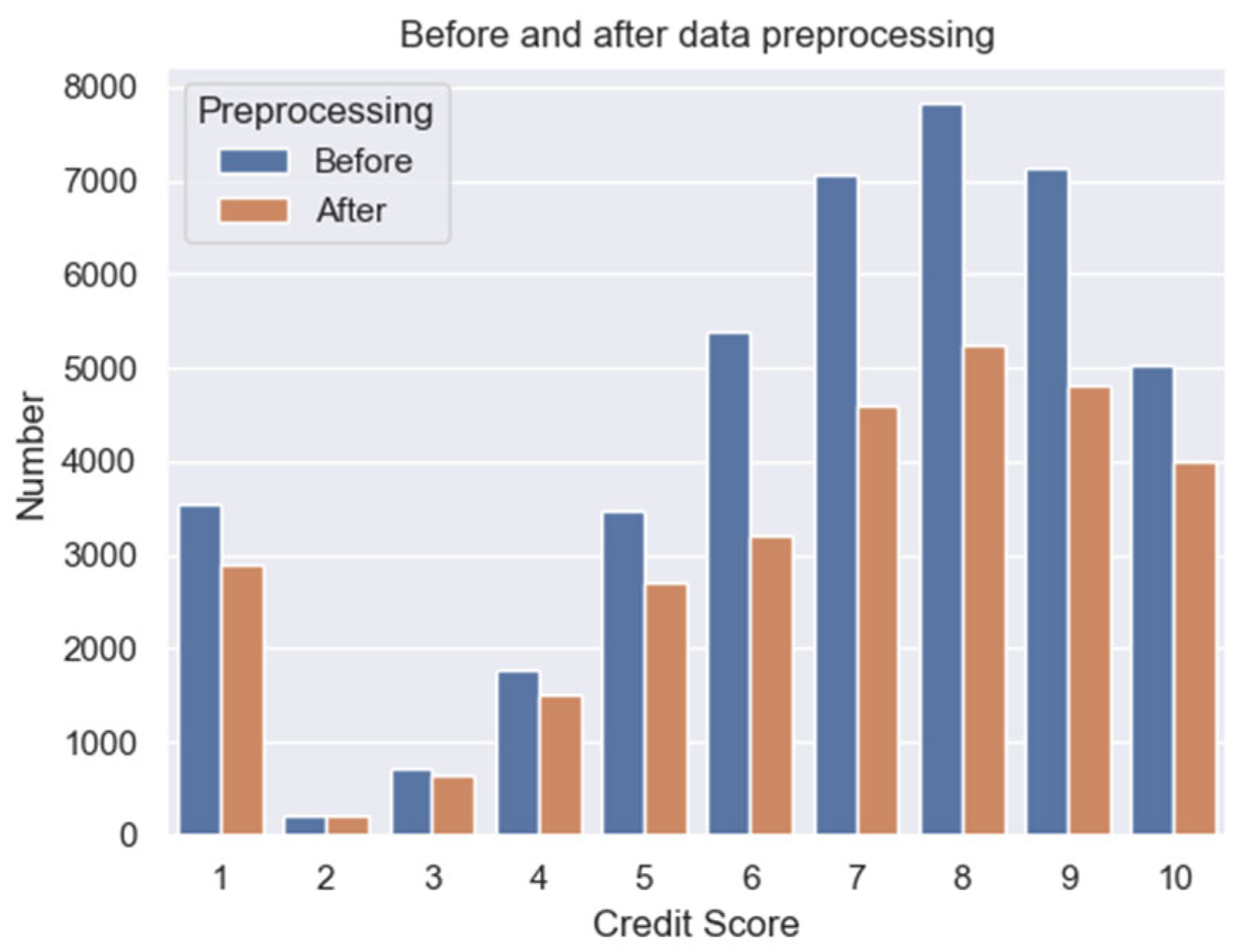
After evaluating the raw data, preprocessing steps were applied to the dataset. Samples with missing values and outliers in the features related to payment habits were removed. Duplicate records were handled in two ways: (1) all samples with different values were deleted, (2) samples with the same values were retained only once. Given that the data source has a relational structure, the dataset was also evaluated in terms of data structure and quality. Records that did not correspond to any institution, product, and invoice type were deleted. After the dataset was cleaned of defective data, the normalization and feature selection processes were performed. The class label distribution before and after the preprocessing step is shown in Figure 2. After preprocessing, the dataset consists of 29,817 samples.

In this study, the ANOVA F-Test, chi-square, and mutual information were used as feature selection methods; SMOTE was also chosen as the oversampling method. After feature selection, the dataset was trained by balancing with SMOTE and then tests were performed. All the classification algorithms in Table 6 were also used in this step. The best results were obtained with the EXT classification method. The most successful results based on feature selection method are presented in

Table 7. Best Results Based on Feature Selection Method.

FS	Selected Features	Sampling	Classification	ACC (±)	PRE (±)	REC (±)	F1 (±)	F2 (±)	AUC (±)
ANOVA F-Test	GENDER, AGE, INVOICE_TYPE, CASH_PERCENTAGE, NUMBER_OF_INVOICES_PAID, TOTAL_PAYMENT_AMOUNT, LATEST_PAYMENT_RATE, AVG_DAYS_PAID_LATE, AVG_DAYS_PAID_EARLY, NUMBER_OF_INVOICE_TYPES	SMOTE	EXT	80.49 ± 1.12	79.89 ± 1.25	80.42 ± 1.07	79.83 ± 1.18	80.11 ± 1.14	97.04 ± 0.85
Chi-square	GENDER, AGE, PRODUCT_CODE, INVOICE_TYPE, CASH_PERCENTAGE, NUMBER_OF_INVOICES_PAID, LATEST_PAYMENT_RATE, AVG_DAYS_PAID_LATE, AVG_DAYS_PAID_EARLY, NUMBER_OF_INVOICE_TYPES	SMOTE	EXT	75.88 ± 1.45	75.89 ± 1.32	75.88 ± 1.36	75.39 ± 1.48	75.58 ± 1.42	96.01 ± 0.97
Mutual Information	AGE PRODUCT_CODE CASH_PERCENTAGE NUMBER_OF_INVOICES_PAID TOTAL_PAYMENT_AMOUNT PAYMENT_AMOUNT_AVG LATEST_PAYMENT_RATE AVG_DAYS_PAID_LATE AVG_DAYS_PAID_EARLY NUMBER_OF_INVOICE_TYPES	SMOTE	EXT	79.09 ± 1.21	78.40 ± 1.30	78.97 ± 1.15	78.35 ± 1.19	78.58 ± 1.17	96.73 ± 0.90

.

Table 7 shows that all three feature selection methods yielded the best performance by selecting 10 features. ANOVA method; PRODUCT_CODE and PAYMENT_AMOUNT_AVG, Chi-square method; TOTAL_PAYMENT_AMOUNT and PAYMENT_AMOUNT_AVG, mutual information method; GENDER and INVOICE_TYPE features were not selected. When the preferences of the feature selection methods are considered, the CASH_PERCENTAGE, LATEST_PAYMENT_RATE, AVG_DAYS_PAID_LATE, AVG_DAYS_PAID_EARLY, and NUMBER_OF_INVOICE_TYPES features indicating payment habits were used in each method and were found to be important parameters. The AGE feature indicating the age of the customer was also used in all methods. The best overall performance was achieved using the EXT classification algorithm. Among the feature selection methods, the ANOVA F-test yielded the most successful results across all evaluation metrics. Specifically, this configuration achieved an accuracy of 80.49% ± 1.12 and an AUC of 97.04% ± 0.85. The precision, recall, F1, and F2 scores were also higher than those of the other models. In addition, the relatively low standard deviations observed indicate high stability and consistency across cross-validation folds.

4.3. Evaluation of the Model with XAI Methods

As seen in Table 7, the best performance was obtained using the ANOVA FS, SMOTE sampling, and EXT classification algorithms. In this step, LIME and SHAP, both XAI methods, were employed to transform the successful model into an explainable and interpretable form. The flow of this proposed model is summarized in Figure 3.

The best ML model was interpreted by performing XAI analysis using the LIME and SHAP methods.

4.3.1. Explaining the Best Model with LIME

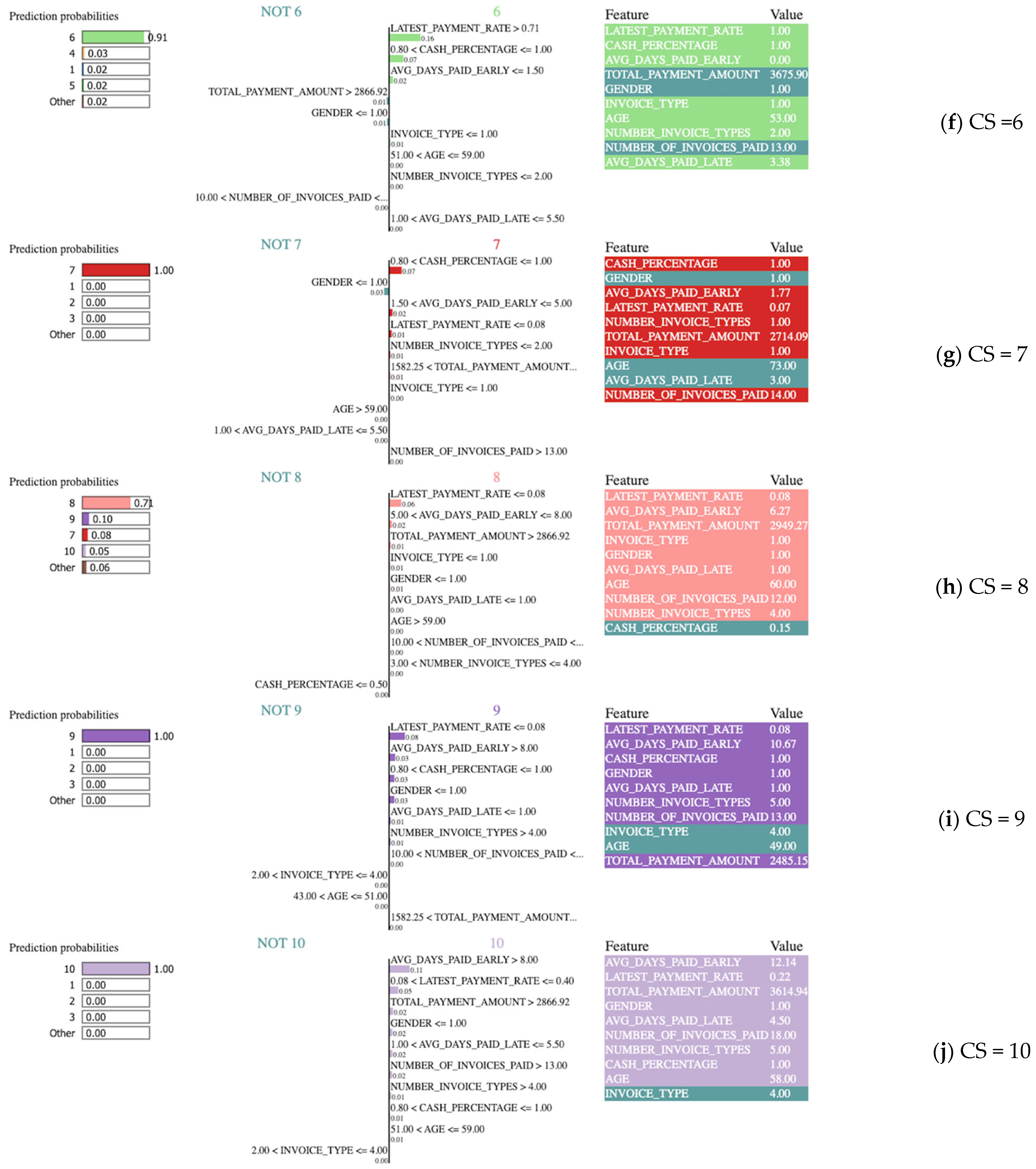
LIME is a method that enables the examination of the prediction probabilities for the relevant class value of the selected examples from the dataset, along with the features and values used to make this prediction. In this study, random examples belonging to 10 classes that were correctly predicted were selected, and the LIME outputs shown in Figure 4 were included. These outputs provide insight into the decision-making process of the model while making predictions for the selected sample. The LIME results consist of three parts: (1) model predictions for the relevant example, (2) contributions of the features, and (3) actual values of the features. In Figure 4, a sample was selected for each CS, and the corresponding LIME outputs were examined.

According to Figure 4a, the model predicted “1” for the selected sample at a rate of 100%. The graph in the second area summarizes the decision status according to the values in the selected sample while the model predicted “1”. The features listed under the “NOT 1” heading in green are the features indicating that the model is not “1”. The features listed under the “1” heading in blue are the features contributing to the probability of the model being “1” while making the prediction. When examining the model, the five most important features identified are: cash payment percentage, late payment rate, gender, number of invoice types, and number of paid invoices. According to the model, a cash payment percentage of less than or equal to 0.50, female gender, the number of paid invoices being 10, and the number of paid invoices being 10–13 played the most important roles in the prediction. A late payment rate of 0.08 and 0.40, along with a number of invoice types greater than 4 are the features contributing to the model prediction not being “1”. The third column shows the real values of the features in the selected sample.

The estimate for the sample whose LIME output is given in Figure 4b is “2” at 100%. The most significant features contributing to this prediction are a cash payment percentage between 0.50 and 0.80, a late payment rate greater than 0.71, male gender, an average number of days paid late greater than 12.33, and an age range from 43 to 51. The average number of days paid early and the number of invoices paid have a negative effect on the estimate.

According to the output in Figure 4c, the estimate is definitely “3”. The most important features contributing to this prediction include a late payment rate greater than 0.71, an age of less than 43, an average number of days paid early of less than 1.5, and male gender. The cash payment percentage and total payment amount features contributed to the fact that the model estimate is not “3”.

When Figure 4d is examined, it is seen that the estimate is “4”. The most important features used to make this estimate are highlighted in orange. The three key features are cash payment percentage being less than or equal to 0.80, the average number of days paid early being less than 1.5, and male gender. The overdue payment rate, average number of days paid late, and total payment amount are the features that the model does not use when making the “4” decision.

The selected sample in Figure 4e belongs to class “5” with a rate of 86%, followed by class “6” with a rate of 8%, class “1” with a rate of 3%, and class “4” with a rate of 2%. When estimating for class “5”, the most important features are a cash payment percentage between 0.8 and 1, a late payment rate greater than 0.71, an average number of days paid early less than 1.50, and male gender. The average number of days paid late, the number of invoices paid, the total payment amount, and the age features contribute to the probability that the selected sample belongs to the other classes.

In Figure 4f, the model’s prediction is “6” at a rate of 91%. Based on the features in this example, the prediction belongs to class “4” at a rate of 3% and classes ”1”, “5”, or other at a rate of 2%.

In the sample shown in Figure 4g, the model predicts class “7” with 100% confidence. The most important features contributing to this prediction include cash payment percentage in the range of 0.80 to 1, an average early payment day in the range 1.50–5, a late payment rate less than or equal to 0.08, the number of invoice types being less than 2, and a total payment amount ranging from 1582.25–2866.92. The features and values given under the heading “NOT 7” are used for estimating classes other than “7”.

In Figure 4h, the model predicted “8” with a probability of 71%. The selected sample could belong to “9” with a probability of 10%, class “7” with a probability of 8%, class “10” with a probability of 5%, and other classes with a probability of 6%. The features that enable the model to predict “8” include a late payment rate less than 0.08, an average early payment period between 5–8 days, a total payment amount greater than 2866.92, the bill type electricity, and male gender.

In Figure 4i, the model made a prediction for class “9” with 100% probability. The most important features influencing this prediction include the late payment rate, average number of days paid early, cash payment percentage, gender, average number of days paid late, and number of invoice types. In contrast, the invoice type internet and an age range from 43 to 51 did not contribute to the prediction.

For the example in Figure 4j, the model made an estimate of “10”. The most important features contributing to this prediction are the average number of days paid early, late payment rate, total payment amount, and gender. The invoice type, GSM, was not used in this estimate.

When drawing inferences about explainability and interpretability via LIME, more reliable explanations and interpretations can be achieved by increasing the variety of selected samples and labels. Efficient outputs can be obtained by abstracting the end user from the complex machine learning model used.

4.3.2. Explaining the Best Model with SHAP

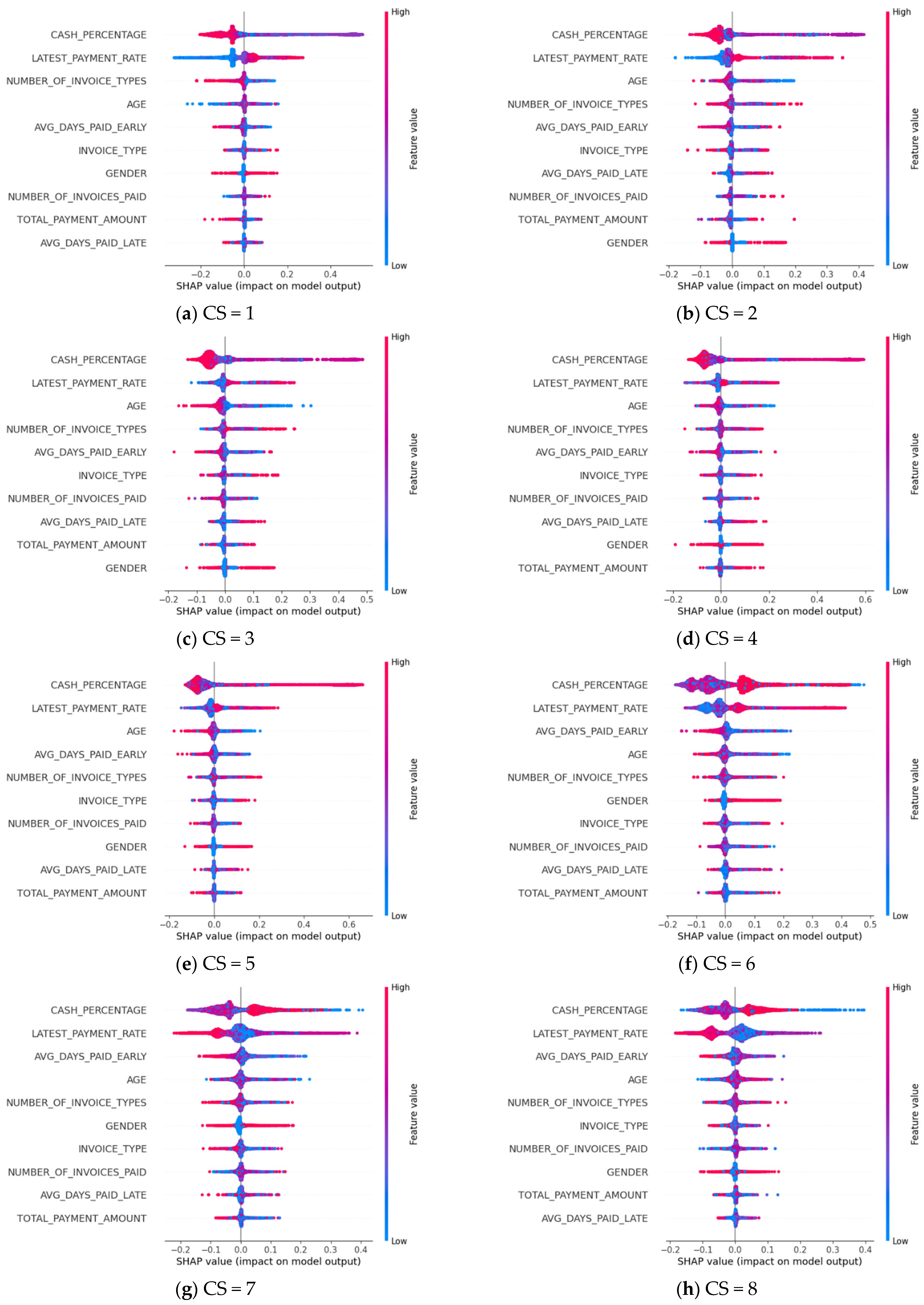
The SHAP approach offers a more detailed overview of the impact of each feature on a specific label. The feature importance can be examined for each label value. In our study, there are 10 label values ranging from 1 to 10, where 1 represents the worst credit score and 10 the best. Feature importance graphs for each label are prepared and displayed in Figure 5.

The details of SHAP outputs in Figure 5 are summarized as follows:

• The y-axis represents the features used in the model training. The features that have the most impact on the result are listed from top to bottom in order of their impact on the result, with the most significant features at the top.
• Each point on the X-axis represents a calculated Shapley value. Positive values on the X-axis are values that contribute positively to the corresponding label value estimate, while negative values indicate a negative contribution to the estimate.
• The colors of the points on the X-axis help to interpret the numerical value of the data. As the color transitions from blue to red, it signifies an increase in the numerical value.
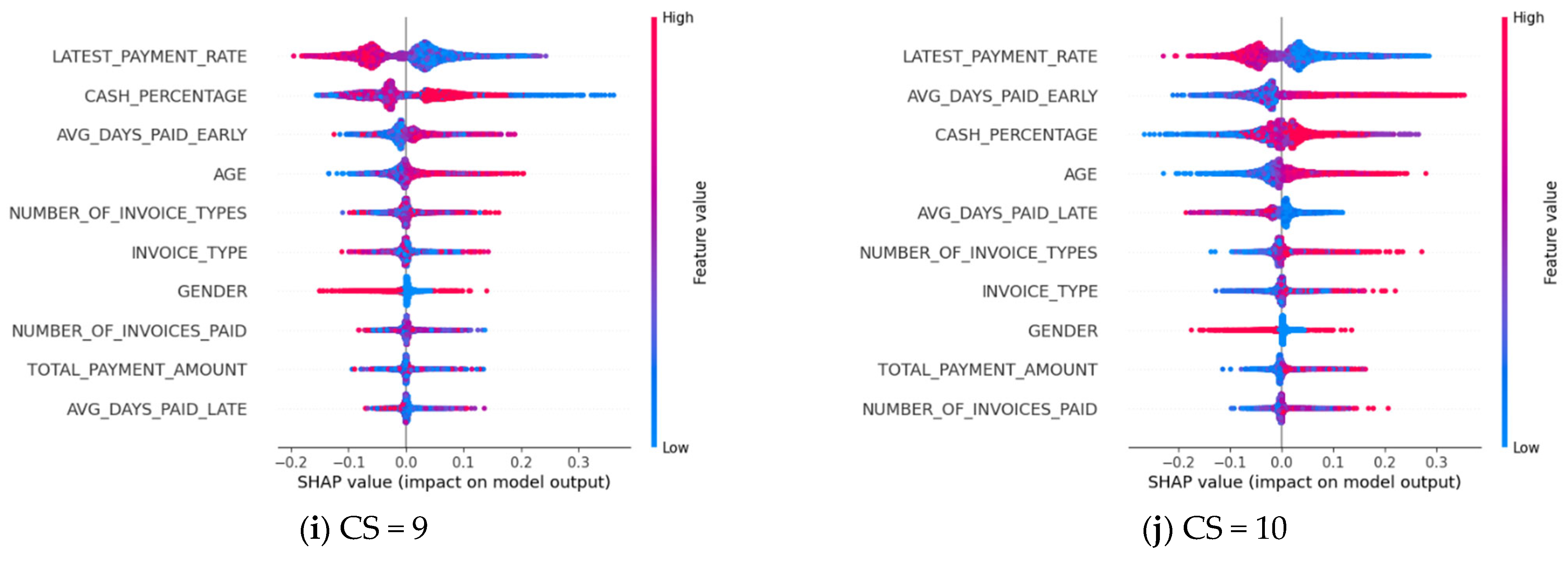
• The two most important features in estimating customers with a credit score between 1–8 are cash payment percentage and late payment rate. It is evident that as the credit score value increases, so does the cash payment percentage. When looking at customers in this range, it can be concluded that those who pay their bills late have lower credit scores.
• Examining the graphs for customers with credit scores of 9 and 10 reveals that the late payment rate is the most important feature. It can be said that the people with the highest scores do not have a habit of incurring overdue payments. In addition, these people tend to pay their bills before the due date and mostly make their payments in cash.
• The graphs for all credit scores indicate that the number of different types of bills paid by the customer, the type of bill, and the age of the customer are among the important features.

When examining the LIME and SHAP outputs, the following conclusions can be drawn:

• Customers with a habit of overdue payments have lower credit scores.
• Customers with high credit scores prefer to pay their bills in cash.
• As the number of days paid early increases, the credit score improves.
• Each feature has a different level of importance in different labels.
• The number of invoices for different types of bills in the relevant payment institution emerges as an important feature.

5. Conclusions

The dataset analyzed in this study was generated from invoice payment data belonging to a payment institution in Turkey. Using invoice payment transactions, person-based payment habits were created and combined with real credit scores to obtain the final dataset that is the subject of this study. The dataset has a 10-class and unbalanced structure. First, the raw dataset was classified using various algorithms, including LR, DT, SVM, RF, EXT, NB, and MLP. Following this, preprocessing steps were applied to clean the data by removing missing values, outliers, and low-quality samples. The dataset was then normalized using min-max scaling and subjected to feature selection by means of the ANOVA F-test, chi-square, and mutual information methods. The dataset was balanced with the SMOTE method and the classification performances were re-evaluated. The highest performance was achieved in the model created with the ANOVA F-test feature selection, SMOTE oversampling, and EXT classification methods. This model was examined and evaluated in terms of explainability and interpretability with the LIME and SHAP XAI techniques.

This study emphasizes the importance of the data preprocessing step. Missing values and outlier data in the dataset were identified and removed. In addition, data quality and consistency were assessed. Samples sourced from a relational database were analyzed to eliminate data lacking relational counterparts or containing incorrect relationships. This thorough cleaning process ensured more accurate training of the machine learning model and ultimately improved performance.

One of the most important parameters of ML models is feature selection. With the feature selection methods used in this study, features that do not contribute to the model were removed from the dataset and the most efficient feature set was used.

Given that the dataset has a multi-class and imbalanced structure, it was trained by balancing it using the artificial sampling method. The exploration and application of these artificial sampling techniques to address data imbalance, a common issue in real CRA datasets, will be insightful for future studies.

In the tests conducted in this study, tree-based classification algorithms demonstrated high performance in CRA. Performance analyses were run using various evaluation metrics, including ACC, PRE, REC, F1 score, F2 score, and AUC to assess reliability. The best performance was achieved with the EXT algorithm. ACC was measured as 80.49% and AUC as 97.04%. In addition, PRE was 79.89, REC was 80.42, F1 score was 79.83%, and F2 score was 80.11%.

It is crucial for systems with complex models to be transparent, explainable, and interpretable. For this reason, the model with the best performance was transformed into an explainable form using the LIME and SHAP in XAI methods, and the model was made understandable and interpretable for everyone. In addition, the analysis highlighted the feature importance for different classes and illustrated the decision-making path followed by the model.

Our study presents a model that can be an alternative to the traditional CRA systems calculated based on credit history data. This model, developed using data from people’s bill payment habits, can be employed as a risk assessment tool for individuals without a credit history or as a supplementary resource for those with existing credit scores. The incorporation of XAI methods in the study can be used as an important parameter for credit providers. Since credit providers can transparently observe the decision-making process and underlying logic of the model, the model can contribute positively to the process in terms of control and security. The transformation of the machine learning model into an explainable and interpretable format addresses concerns related to reliability, transparency, fairness, and ethics—key principles of XAI.

In this study, it has been shown that data preprocessing steps, tree-based classification algorithms, feature selection, and data balancing can significantly enhance performance in multi-class and unbalanced CRA datasets. Our study has provided evaluations indicating that various debt payment behaviors or habits can serve as valuable references for credit risk assessment. Additionally, we emphasize the importance of using XAI methods, particularly for financial models where sensitivity and reliability are paramount. Our study offers a suggestion for abstracting end users from complex machine learning models while delivering understandable and interpretable outputs. The model we propose can be easily applied in real life and put to use by banks or financial institutions.

6. Future Works

In our study, a dataset obtained by combining bill payment habits and real credit scores was used. The most efficient model was obtained by applying various ML methods to a multi-class and imbalanced dataset. This model was transformed into a transparent form using LIME and SHAP methods, creating a hybrid approach.

Future studies can focus on the following topics:

• Alternative datasets can be used for CRA.
• Other sampling or weighting methods can be used for unbalanced datasets.
• Studies on hyperparameter optimization can be conducted to further enhance model performance and evaluate how changes in hyperparameters impact results.
• Efficiency can be increased by using different feature selection and dimension reduction methods for CRA.
• Research can be conducted on the contribution of different approaches, such as deep learning, to performance.
• Reference can be made to studies on XAI approaches for transparent ML models.

References

- Tripathi, D.; Shukla, A.K.; Reddy, B.R.; Bopche, G.S.; Chandramohan, D. Credit Scoring Models Using Ensemble Learning and Classification Approaches: A Comprehensive Survey. Wirel. Pers. Commun 2022, 123, 785–812. [Google Scholar] [CrossRef]
- Thomas, L.; Crook, J.; Edelman, D. Chapter 1: The History and Philosophy of Credit Scoring. In Credit Scoring and Its Applications, 2nd ed.; Mathematics in Industry; Society for Industrial and Applied Mathematics: Philadelphia, PA, USA, 2017; pp. 1–10. [Google Scholar] [CrossRef]
- Arya, S.; Eckel, C.; Wichman, C. Anatomy of the credit score. J. Econ. Behav. Organ. 2013, 95, 175–185. [Google Scholar] [CrossRef]
- Avery, R.B.; Brevoort, K.P.; Canner, G.B. Credit Scoring and Its Effects on the Availability and Affordability of Credit. J. Consum. Aff. 2009, 43, 516–537. [Google Scholar] [CrossRef]
- Lessmann, S.; Baesens, B.; Seow, H.-V.; Thomas, L.C. Benchmarking state-of-the-art classification algorithms for credit scoring: An update of research. Eur. J. Oper. Res. 2015, 247, 124–136. [Google Scholar] [CrossRef]
- Luo, C.; Wu, D.; Wu, D. A deep learning approach for credit scoring using credit default swaps. Eng. Appl. Artif. Intell. 2017, 65, 465–470. [Google Scholar] [CrossRef]
- Dumitrescu, E.; Hué, S.; Hurlin, C.; Tokpavi, S. Machine learning for credit scoring: Improving logistic regression with non-linear decision-tree effects. Eur. J. Oper. Res. 2022, 297, 1178–1192. [Google Scholar] [CrossRef]
- Zhao, S.; Fujita, H. Predicting the Listing Status of Chinese Listed Companies Using Twin Multi-class Classification Support Vector Machine. In Advances and Trends in Artificial Intelligence. From Theory to Practice; Wotawa, F., Friedrich, G., Pill, I., Koitz-Hristov, R., Ali, M., Eds.; Lecture Notes in Computer Science; Springer International Publishing: Cham, Switzerland, 2019; pp. 50–62. [Google Scholar] [CrossRef]
- Kruppa, J.; Schwarz, A.; Arminger, G.; Ziegler, A. Consumer credit risk: Individual probability estimates using machine learning. Expert Syst. Appl. 2013, 40, 5125–5131. [Google Scholar] [CrossRef]
- Appel, A.P.; Oliveira, V.; Lima, B.; Malfatti, G.L.; de Santana, V.F.; de Paula, R. Optimize Cash Collection: Use Machine learning to Predicting Invoice Payment. arXiv 2019, arXiv:1912.10828. [Google Scholar] [CrossRef]
- Boughaci, D.; Alkhawaldeh, A.A.K. Appropriate machine learning techniques for credit scoring and bankruptcy prediction in banking and finance: A comparative study. Risk Decis. Anal. 2020, 8, 15–24. [Google Scholar] [CrossRef]
- Xia, Y.; Zhao, J.; He, L.; Li, Y.; Niu, M. A novel tree-based dynamic heterogeneous ensemble method for credit scoring. Expert Syst. Appl. 2020, 159, 113615. [Google Scholar] [CrossRef]
- Wu, Y.; Pan, Y. Application Analysis of Credit Scoring of Financial Institutions Based on Machine Learning Model. Complexity 2021, 2021, e9222617. [Google Scholar] [CrossRef]
- Niu, B.; Ren, J.; Li, X. Credit Scoring Using Machine Learning by Combing Social Network Information: Evidence from Peer-to-Peer Lending. Information 2019, 10, 397. [Google Scholar] [CrossRef]
- De Cnudde, S.; Moeyersoms, J.; Stankova, M.; Tobback, E.; Javaly, V.; Martens, D. What does your Facebook profile reveal about your creditworthiness? Using alternative data for microfinance. J. Oper. Res. Soc. 2019, 70, 353–363. [Google Scholar] [CrossRef]
- Djeundje, V.B.; Crook, J.; Calabrese, R.; Hamid, M. Enhancing credit scoring with alternative data. Expert Syst. Appl. 2021, 163, 113766. [Google Scholar] [CrossRef]
- Bücker, M.; Szepannek, G.; Gosiewska, A.; Biecek, P. Transparency, auditability, and explainability of machine learning models in credit scoring. J. Oper. Res. Soc. 2022, 73, 70–90. [Google Scholar] [CrossRef]
- Nikolinakos, N.T. The Proposed Artificial Intelligence Act and Subsequent ‘Compromise’ Proposals: Commission, Council, Parliament. In EU Policy and Legal Framework for Artificial Intelligence, Robotics and Related Technologies—The AI Act; Nikolinakos, N.T., Ed.; Springer International Publishing: Cham, Switzerland, 2023; pp. 327–741. [Google Scholar] [CrossRef]
- Talaat, F.M.; Aljadani, A.; Badawy, M.; Elhosseini, M. Toward interpretable credit scoring: Integrating explainable artificial intelligence with deep learning for credit card default prediction. Neural Comput. Appl. 2024, 36, 4847–4865. [Google Scholar] [CrossRef]
- El Qadi, A.; Trocan, M.; Díaz-Rodríguez, N.; Frossard, T. Feature contribution alignment with expert knowledge for artificial intelligence credit scoring. SIViP 2023, 17, 427–434. [Google Scholar] [CrossRef]
- Heng, Y.S.; Subramanian, P. A Systematic Review of Machine Learning and Explainable Artificial Intelligence (XAI) in Credit Risk Modelling. In Proceedings of the Future Technologies Conference (FTC) 2022, Volume 1; Arai, K., Ed.; Springer International Publishing: Cham, Switzerland, 2023; pp. 596–614. [Google Scholar] [CrossRef]
- Abedin, M.Z.; Guotai, C.; Hajek, P.; Zhang, T. Combining weighted SMOTE with ensemble learning for the class-imbalanced prediction of small business credit risk. Complex Intell. Syst. 2023, 9, 3559–3579. [Google Scholar] [CrossRef]
- Lenka, S.R.; Bisoy, S.K.; Priyadarshini, R.; Sain, M. Empirical Analysis of Ensemble Learning for Imbalanced Credit Scoring Datasets: A Systematic Review. Wirel. Commun. Mob. Comput. 2022, 2022, 6584352. [Google Scholar] [CrossRef]
- Zhu, M.; Zhang, Y.; Gong, Y.; Xu, C.; Xiang, Y. Enhancing Credit Card Fraud Detection A Neural Network and SMOTE Integrated Approach. arXiv 2024, arXiv:2405.00026. [Google Scholar] [CrossRef]
- Xia, Y.; Liu, C.; Li, Y.; Liu, N. A boosted decision tree approach using Bayesian hyper-parameter optimization for credit scoring. Expert Syst. Appl. 2017, 78, 225–241. [Google Scholar] [CrossRef]
- Zhou, G.; Zhang, Y.; Luo, S. P2P Network Lending, Loss Given Default and Credit Risks. Sustainability 2018, 10, 1010. [Google Scholar] [CrossRef]
- Chen, Q.; Tsai, S.-B.; Zhai, Y.; Chu, C.-C.; Zhou, J.; Li, G.; Zheng, Y.; Wang, J.; Chang, L.-C.; Hsu, C.-F. An Empirical Research on Bank Client Credit Assessments. Sustainability 2018, 10, 1406. [Google Scholar] [CrossRef]
- Edalo, C.; Diallo, R.; Awe, O.O. Machine Learning Prediction of Multiclass Credit Score Classification. In Practical Statistical Learning and Data Science Methods: Case Studies from LISA 2020 Global Network, USA; Awe, O.O., Vance, E.A., Eds.; Springer International Publishing: Cham, Switzerland, 2025; pp. 413–433. [Google Scholar] [CrossRef]
- Moscato, V.; Picariello, A.; Sperlí, G. A benchmark of machine learning approaches for credit score prediction. Expert Syst. Appl. 2021, 165, 113986. [Google Scholar] [CrossRef]
- Ariza-Garzón, M.J.; Arroyo, J.; Caparrini, A.; Segovia-Vargas, M.-J. Explainability of a Machine Learning Granting Scoring Model in Peer-to-Peer Lending. IEEE Access 2020, 8, 64873–64890. [Google Scholar] [CrossRef]
- Zhao, Z.; Bai, T. Financial Fraud Detection and Prediction in Listed Companies Using SMOTE and Machine Learning Algorithms. Entropy 2022, 24, 1157. [Google Scholar] [CrossRef] [PubMed]
- Gramegna, A.; Giudici, P. SHAP and LIME: An Evaluation of Discriminative Power in Credit Risk. Front. Artif. Intell. 2021, 4, 752558. [Google Scholar] [CrossRef]
- Nallakaruppan, M.K.; Balusamy, B.; Shri, M.L.; Malathi, V.; Bhattacharyya, S. An Explainable AI framework for credit evaluation and analysis. Appl. Soft Comput. 2024, 153, 111307. [Google Scholar] [CrossRef]
- Naramala, V.K.; Ravipudi, L.P.; Bhavanam, S.P.R.; Pokuri, V.N.; Kumar, S.V.P.; Kishore, V.K. Prediction of Credit Card Fraud detection using Extra Tree Classifier and Data Balancing Methods. In Proceedings of the 2024 IEEE 3rd World Conference on Applied Intelligence and Computing (AIC), Gwalior, India, 27–28 July 2024; pp. 722–728. [Google Scholar] [CrossRef]
- Jovanovic, Z.; Hou, Z.; Biswas, K.; Muthukkumarasamy, V. Robust integration of blockchain and explainable federated learning for automated credit scoring. Comput. Netw. 2024, 243, 110303. [Google Scholar] [CrossRef]
- Bastos, J.A.; Matos, S.M. Explainable models of credit losses. Eur. J. Oper. Res. 2022, 301, 386–394. [Google Scholar] [CrossRef]
- Alblooshi, M.; Alhajeri, H.; Almatrooshi, M.; Alaraj, M. Unlocking Transparency in Credit Scoring: Leveraging XGBoost with XAI for Informed Business Decision-Making. In Proceedings of the 2024 International Conference on Artificial Intelligence, Computer, Data Sciences and Applications (ACDSA), Victoria, Seychelles, 1–2 February 2024; pp. 1–6. [Google Scholar] [CrossRef]
- Pyle, D. Data Preparation for Data Mining; Morgan Kaufmann: Burlington, MA, USA, 1999. [Google Scholar]
- Statistical Analysis with Missing Data, Third Edition|Wiley Series in Probability and Statistics. Available online: https://onlinelibrary.wiley.com/doi/book/10.1002/9781119482260 (accessed on 19 February 2024).
- Zhu, X.; Wu, X. Class Noise vs. Attribute Noise: A Quantitative Study. Artif. Intell. Rev. 2004, 22, 177–210. [Google Scholar] [CrossRef]
- Guyon, I.; Elisseeff, A. An introduction to variable and feature selection. J. Mach. Learn. Res. 2003, 3, 1157–1182. [Google Scholar]
- Siham, A.; Sara, S.; Abdellah, A. Feature selection based on machine learning for credit scoring: An evaluation of filter and embedded methods. In Proceedings of the 2021 International Conference on INnovations in Intelligent SysTems and Applications (INISTA), Kocaeli, Turkey, 25–27 October 2021; pp. 1–6. [Google Scholar] [CrossRef]
- Field, A. Discovering Statistics Using IBM SPSS Statistics; SAGE Publications: New York, NY, USA, 2024. [Google Scholar]
- Bro, R.; Methods, A.K. Principal component analysis. Anal. Methods 2014, 6, 2812–2831. [Google Scholar] [CrossRef]
- De Schutter, B.; van den Boom, T.J.J. Model predictive control for max-min-plus-scaling systems. In Proceedings of the Proceedings of the 2001 American Control Conference. (Cat. No.01CH37148), Arlington, VA, USA, 25–27 June 2001; Volume 1, pp. 319–324. [Google Scholar] [CrossRef]
- Yap, B.W.; Rani, K.A.; Rahman, H.A.A.; Fong, S.; Khairudin, Z.; Abdullah, N.N. An Application of Oversampling, Undersampling, Bagging and Boosting in Handling Imbalanced Datasets. In Proceedings of the First International Conference on Advanced Data and Information Engineering (DaEng-2013); Herawan, T., Deris, M.M., Abawajy, J., Eds.; Lecture Notes in Electrical Engineering; Springer: Singapore, 2014; pp. 13–22. [Google Scholar] [CrossRef]
- Menardi, G.; Torelli, N. Training and assessing classification rules with imbalanced data. Data Min. Knowl. Discov. 2014, 28, 92–122. [Google Scholar] [CrossRef]
- Chawla, N.V.; Bowyer, K.W.; Hall, L.O.; Kegelmeyer, W.P. SMOTE: Synthetic Minority Over-sampling Technique. J. Artif. Intell. Res. 2002, 16, 321–357. [Google Scholar] [CrossRef]
- He, H.; Bai, Y.; Garcia, E.A.; Li, S. ADASYN: Adaptive synthetic sampling approach for imbalanced learning. In Proceedings of the 2008 IEEE International Joint Conference on Neural Networks (IEEE World Congress on Computational Intelligence), Hong Kong, China, 1–8 June 2008; pp. 1322–1328. [Google Scholar] [CrossRef]
- Kang, Q.; Chen, X.; Li, S.; Zhou, M. A Noise-Filtered Under-Sampling Scheme for Imbalanced Classification. IEEE Trans. Cybern. 2017, 47, 4263–4274. [Google Scholar] [CrossRef]
- Wilson, D.L. Asymptotic Properties of Nearest Neighbor Rules Using Edited Data. IEEE Trans. Syst. Man Cybern. 1972, SMC-2, 408–421. [Google Scholar] [CrossRef]
- Tomek, I. Two Modifications of CNN. IEEE Trans. Syst. Man Cybern. 1976, SMC-6, 769–772. [Google Scholar] [CrossRef]
- Batista, G.E.A.P.A.; Prati, R.C.; Monard, M.C. A study of the behavior of several methods for balancing machine learning training data. ACM SIGKDD Explor. Newsl. 2004, 6, 20–29. [Google Scholar] [CrossRef]
- Batista, G.; Bazzan, A.; Monard, M.-C. Balancing Training Data for Automated Annotation of Keywords: A Case Study. In Proceedings of the Workshop on Bioinformatics, Macaé, RJ, Brazil, 3–5 December 2003; pp. 10–18. [Google Scholar]
- Kotsiantis, S.B. Decision trees: A recent overview. Artif. Intell. Rev. 2013, 39, 261–283. [Google Scholar] [CrossRef]
- Breiman, L. Random Forests. Mach. Learn. 2001, 45, 5–32. [Google Scholar] [CrossRef]
- Geurts, P.; Ernst, D.; Learn, L. Extremely randomized trees. Mach. Learn. 2006, 63, 3–42. [Google Scholar] [CrossRef]
- Pattern Recognition and Machine Learning. Available online: https://link.springer.com/book/9780387310732 (accessed on 15 February 2024).
- Rennie, J.D.M.; Shih, L.; Teevan, J.; Karger, D.R. Tackling the Poor Assumptions of Naive Bayes Text Classifiers. In Proceedings of the 20th International Conference on Machine Learning (ICML-03), Washington, DC, USA, 21–24 August 2003; pp. 616–623. [Google Scholar]
- Tang, J.; Deng, C.; Huang, G.-B. Extreme Learning Machine for Multilayer Perceptron. IEEE Trans. Neural Netw. Learn. Syst. 2016, 27, 809–821. [Google Scholar] [CrossRef]
- Zhang, C.; Pan, X.; Li, H.; Gardiner, A.; Sargent, I.; Hare, J.; Atkinson, P.M. A hybrid MLP-CNN classifier for very fine resolution remotely sensed image classification. ISPRS J. Photogramm. Remote Sens. 2018, 140, 133–144. [Google Scholar] [CrossRef]
- Fushiki, T. Estimation of prediction error by using K-fold cross-validation. Stat. Comput. 2011, 21, 137–146. [Google Scholar] [CrossRef]
- Prasetiyo, B.; Alamsyah; Muslim, M.A.; Baroroh, N. Evaluation performance recall and F2 score of credit card fraud detection unbalanced dataset using SMOTE oversampling technique. J. Phys. Conf. Ser. 2021, 1918, 042002. [Google Scholar] [CrossRef]
- Fawcett, T. An introduction to ROC analysis. Pattern Recognit. Lett. 2006, 27, 861–874. [Google Scholar] [CrossRef]
- Carvalho, D.V.; Pereira, E.M.; Cardoso, J.S. Machine Learning Interpretability: A Survey on Methods and Metrics. Electronics 2019, 8, 832. [Google Scholar] [CrossRef]
- Ribeiro, M.T.; Singh, S.; Guestrin, C. ‘Why Should I Trust You?’: Explaining the Predictions of Any Classifier. arXiv 2016, arXiv:1602.04938. [Google Scholar] [CrossRef]
- Arrow, K.J.; Barankin, E.W.; Blackwell, D.; Bott, R.; Dalkey, N.; Dresher, M.; Gale, D.; Gillies, D.B.; Glicksberg, I.; Gross, O.; et al. Contributions to the Theory of Games (AM-28), Volume II; Princeton University Press: Princeton, NJ, USA, 1953; Available online: https://www.jstor.org/stable/j.ctt1b9x1zv (accessed on 27 February 2024).
- Lundberg, S.M.; Lee, S.-I. A Unified Approach to Interpreting Model Predictions. In Advances in Neural Information Processing Systems; Curran Associates, Inc.: Red Hook, NY, USA, 2017; Available online: https://papers.nips.cc/paper_files/paper/2017/hash/8a20a8621978632d76c43dfd28b67767-Abstract.html (accessed on 27 February 2024).
- Rodríguez-Pérez, R.; Bajorath, J. Interpretation of machine learning models using shapley values: Application to compound potency and multi-target activity predictions. J. Comput. Aided Mol. Des. 2020, 34, 1013–1026. [Google Scholar] [CrossRef]