Article

Beat the Offers—A Machine-Learning Approach for Predicting Contestants’ Choices and Games’ Outcomes on a TV Quiz Show

Faculty of Electrical Engineering and Computing, University of Zagreb, 10000 Zagreb, Croatia
*
Author to whom correspondence should be addressed.
Appl. Sci. 2025, 15(10), 5722; https://doi.org/10.3390/app15105722
Submission received: 8 April 2025 / Revised: 14 May 2025 / Accepted: 16 May 2025 / Published: 20 May 2025
(This article belongs to the Special Issue Applications of Data Science and Artificial Intelligence)

Abstract

:
Beat the Chasers is a popular UK-originating TV quiz show that premiered in Croatia in 2023. On the show, a contestant challenges a team of up to five chasers with respect to the offers provided by the production. Each offer balances risk and reward, varying in prize money, time advantage, and the number of chasers. In this paper, we first present the dataset obtained by extracting data from the publicly broadcast episodes of Beat the Chasers in Croatia. We then apply various machine-learning models with the goals of predicting (1) which offer a contestant is most likely to select and (2) the game’s outcome. The best-case results suggest that we can successfully do both by reaching an F1-score of 73.6 % for the selected offer prediction and 84.6 % for the game’s outcome prediction. Regarding the feature importance analysis, we identified the contestant’s hometown size, NUTS 2 region, age group, and gender as the most relevant features in the case of the selected offer prediction. As for the outcome prediction, the game-specific features emerged as the most important, namely, the cash builder result, the selected number of chasers, and the chasers’ time in the selected offer.

1. Introduction

The Chase is a popular TV quiz show licensed by ITV Global Entertainment Limited. On each episode, four contestants, who have just met for the first time, aim to beat the chaser (a professional quiz player) and win a specific amount of money. The show has been broadcast in the United Kingdom since 2009, with numerous international versions produced, including the Croatian version, which has been broadcast by Croatian Radiotelevision (Hrvatska radiotelevizija, abbreviated as HRT) since 2013. Because of the show’s immense popularity, several spin-off versions have been created, such as celebrity specials (The Chase: Celebrity Special), for charitable purposes, The Family Chase, where four family members compete together, and, ultimately, Beat the Chasers. The latter, which is the focus of this paper, immediately gained popularity in all markets because of its pronounced dynamics and suspense. The main premise of the show is the inversion of the original concept. Although in The Chase, a team of contestants faces one chaser, in Beat the Chasers, a single contestant faces a team of chasers. The show began airing in 2023.
Although the rules of the game will be explained in detail in Section 3, it is important to mention the offers as one of the main concepts of the quiz. After the initial part of the game (the so-called cash builder), where a contestant answers a maximum of five questions, they challenge a team of up to five chasers, usually professional quizzers, with respect to the offers given by the host. Each offer balances risk and reward, varying in prize money, time advantage, and the number of chasers. During the airing time, it was observed that sometimes the contestants received vastly different offers, despite answering the same number of questions in the first phase of the game (i.e., in the cash builder). Some offers differ significantly in the prize money or the time allocated to the chasers, while others vary only in the order of the chasers.
The motivation behind this study stems from a desire to understand how contestants make decisions regarding the offers presented to them, specifically, how their demographic data and personal traits (i.e., contestants’ profiles) influence their choices and, ultimately, shape the outcome. By applying artificial intelligence methods, deeper insights into the decision-making process could be uncovered, ultimately contributing to a more strategic and informed approach for both the contestants and the show’s producers. From the producers’ perspective, a better understanding of these dynamics could lead to a more engaging show, while contestants could benefit from improved preparation and a more predictable decision-making framework.
The study of human decision making falls within the domain of psychology and has been under extensive research for several decades. Among the most influential contributors to this field are Kahneman and Tversky, whose development of prospect theory fundamentally reshaped the understanding of decision making under risk. One of the key insights of prospect theory is the certainty effect, wherein individuals tend to underweight outcomes with low probabilities and overweight outcomes that are certain [1]. This leads to loss aversion, the principle that losses have a greater psychological impact than equivalent gains, which manifests as risk aversion in scenarios involving potential gains and risk-seeking behavior when faced with potential losses. Additionally, their work highlights that choices are typically evaluated relative to a reference point, rather than in absolute terms [2], and that individuals often ignore elements common to all the alternatives, a tendency known as the isolation effect. Prospect theory was later refined and extended by the same authors [3]. Complementary to this work is their research on human risk assessment [4], which further supplements the complete decision-making picture. On the other hand, Gigerenzer’s approach is similar but different. Together with Goldstein, Gigerenzer introduced a family of fast and frugal heuristics that deliberately ignore a part of the available information and avoid complex integration processes yet often yield effective results in real-world contexts [5]. Gigerenzer argues that the uncertainty and incompleteness, both inherent in heuristic processes, can be advantageous and ultimately lead to better decisions [6]. One of the key insights from this research is the less-is-more effect, which suggests that using fewer cues or less information can sometimes lead to better decisions than more complex approaches. This forms the basis of Gigerenzer’s model of Homo heuristicus, a cognitive agent that features a biased mind and purposefully ignores a part of the available information. Such an agent often performs more efficiently and robustly in uncertain environments than a theoretically unbiased agent relying on exhaustive, resource-intensive methods [7]. Although this is prospective for a study of this kind, we opted not to proceed in that direction, as these aspects are beyond the scope of the present work. Properly addressing psychological factors, such as human decision making, would require more advanced tools, an expanded research framework, and collaboration with experts in other applicable fields.
Instead, this paper aims to investigate several artificial intelligence methods used to predict the course of the game. This research is divided into two main goals: The first part (Section 5.2) seeks to identify which offer a contestant will select based on (1) the contestant’s profile, (2) the contestant’s profile and the cash builder result, and, finally, (3) the contestant’s partial profile (gender, age group, hometown size, and NUTS 2 region). Cases (1) and (2) are separated to determine whether the cash builder results significantly influence contestants’ choices, while case (3) came out as one of the combinations that yielded the best prediction results.
The second part (Section 5.3) of the analysis aims to predict the game’s outcome based on six different feature combinations (i.e., scenarios). The first scenario aims to do so based on only (1) the contestant’s profile, while the second adds (2) the cash builder result, all the offers, and specific chasers within the selected offer alongside the contestant’s profile. The third scenario explores the influence of the contestant’s profile on the outcome by removing the profile from the second scenario, yielding a feature set comprising (3) the cash builder result, all the offers, and specific chasers within the selected offer. The fourth, fifth, and sixth scenarios completely disregard the concepts of a profile and an offer and aim to predict the outcome based on (4) the selected number of chasers and the cash builder result, (5) the selected number of chasers and the chasers’ time in the selected offer, and (6) the selected number of chasers, cash builder result, and chasers’ time in the selected offer.
To sum up, this paper makes the following contributions:
1.
A publicly available dataset for the Croatian version of the Beat the Chasers TV quiz [8];
2.
Tuned machine-learning models for predicting the offers that a contestant is the most likely to select;
3.
Tuned machine-learning models for the game’s outcome prediction;
4.
The identification of the key factors that influence both the selected offer and the game’s outcome prediction.
The rest of the paper is organized as follows. First, in Section 2, we provide a brief overview of the respective field. We then proceed to explain the core rules and propositions of the game in Section 3. The collected dataset is introduced and thoroughly described in Section 4. In Section 5, we describe the methodology and present and discuss the results obtained by applying several machine-learning classifiers for both goals. Finally, the paper is concluded in Section 6.

2. Related Work

In this section, we provide a brief review of the field in terms of data mining and knowledge extraction on quiz-based games and shows. To the best of our knowledge, there has been no published scientific work on either The Chase or Beat the Chasers quizzes. We thus focus on other cases of knowledge extraction in a quizzing context. Because of the limited scientific literature specifically targeting quizzes, we also consider not only the adjacent fields of students’ academic performance and the prediction of sports’ outcomes but also the application of artificial intelligence in consumer behavior analysis, marketing, and gamification.
First, we consider various TV quiz shows. For a show named The Price is Right, Kvam [9] considered various strategies to maximize the winning probability based on the players’ bidding order. They considered the preceding bids of the other players and finally analyzed how confidence can affect the winning probability of a player. Frazen and Pointner analyzed the determinants of successful participation on a popular TV quiz show Who Wants to Be a Millionaire? [10]. The analysis was based on the German instance of the quiz. The authors tested the assumed advantage of social capital in terms of personal networks and human capital in terms of participants’ education. The same TV quiz show was the topic of research of Molino et al. [11,12]. They developed a virtual player for the game, which used various natural language-processing techniques to rank the answers according to several lexical, syntactical, and semantic criteria. These sources also implicitly affirm that the application of the techniques available under the artificial intelligence umbrella to TV quizzes has existed for a not-so-brief period. On the other hand, the authors in [13] explored the use of crowdsourcing and lightweight machine-learning techniques to create a player for the same game. Their system collected answers from a crowd of mobile users and aggregated these responses using various algorithms, including majority voting and confidence-weighted voting. The results demonstrated that by effectively combining crowdsourced data with machine learning, even difficult questions could be answered with a high degree of accuracy, suggesting the feasibility for building a “super player” for question answering. To sum up, research on TV quiz shows so far has primarily focused either on analyzing factors that contributed to or have led to successful participation or on building virtual players, whereas our study concentrates on predicting both in in-game decision making and the final games’ outcomes.
One of the most complete approaches we found involving a contestant’s profile was related not to the TV quiz show but to a reality show. In [14], Lee et al. trained three machine-learning models on demographic and other profile-related data extracted from aired episodes, trying to predict the winner of The Bachelor. The authors stated that they found clear consistency across all three models, which enabled them to pinpoint the specific demographic (e.g., exact age, race, or home region) and in-show achievement parameters that influence the probability of progressing far in the show. The approach taken by the authors in that study to some extent resembles the approach we took in this paper, mainly in terms of the game’s outcome prediction using contestants’ profiles.
Significant work has been conducted within the context of predicting students’ performance. Ofori et al. [15], in their literature-based review of machine-learning algorithms for the prediction of students’ performance, stated contentious results with respect to the selection of a model that best predicts performance. They stated that varying prediction levels may be a result of differences in socioeconomic status or other types of students’ backgrounds, which were not considered when assessing the accuracy of the models. Alhothali et al. [16] performed a survey that examined online learners’ data to predict their outcomes, using machine- and deep-learning techniques. They stated that most studies in the field utilized statistical features, such as the number of downloaded materials and the total time spent on course-related video watching in a given time period. Wu et al. [17] reviewed 83 studies, finding that ensemble-learning models achieved the highest accuracy rate (87.7%), followed by the support-vector-machine (84.3%) approach.
Demographic, academic, and behavioral factors were significant predictors of academic achievement. Rebai et al. [18] applied machine-learning techniques (regression trees and random forests) to Tunisian secondary schools, identifying school size, competition, class size, parental pressure, and the proportion of girls as key performance factors. Random forests additionally revealed the significant roles of the proportion of girls and the school size in improving predictive accuracy and, hence, could influence school efficiency. Similarly, Agyemang et al. [19] found random forests to be the best-performing algorithm for predicting students’ performance, with an accuracy rate of 85.4%. The authors also emphasized challenges such as the lack of standardization in performance metrics, limited model generalization abilities, and potential bias in training data. Finally, Suaza-Medina et al. [20] combined machine-learning algorithms and Shapley values to analyze factors influencing Colombian students’ academic performance. The results showed that the best accuracy was achieved with extreme gradient boosting. Furthermore, according to the Shapley values, the socioeconomic level index, gender, age, region, and school location were identified as key predictors. As shown in related studies on students’ performance in academic contexts, authors typically base their analyses on various subsets of demographic data (as we do in our study), as well as on non-demographic and environmental factors.
The authors in [21] suggested a multilevel heterogeneous predictive model, which yielded an ensemble-learning model for predicting students’ performance and assessments. The authors claimed a predictive accuracy rate of 99.5%. Abiodun and Andrew [22] investigated the prediction of students’ academic performance using ensemble machine-learning algorithms, specifically, random forest, k-nearest neighbors, XGBoost, and a stacked ensemble approach. Their results demonstrated that the stacked ensemble model achieved the best performance. This study builds upon previous work, such as that by Yagci [23] and Ababneh et al. [24], by demonstrating the effectiveness of ensemble methods for improving the accuracy of student performance predictions. Similar to the authors of these studies, we also employed ensemble methods (voting classifiers), which yielded solid, though not the best, results in our case.
Finally, the authors of a review study [25] stated that individuals tend to validly use different multiple-machine-learning models to solve the problems related to predicting students at risk and assessing their performance. Multiple authors have tackled the problem of predicting degree completion with various approaches in terms of machine-learning models and the underlying type of the used data [26,27,28]. The authors in [29] focused on demographic data as predictors of learners’ performance. In this study, we adopted a similar approach by evaluating multiple models to determine which would yield the best results, as we did not have a prior indication of which model might perform optimally.
Machine learning and artificial intelligence have, in general, gained significant traction in the fields of marketing and consumer behavioral analysis. The authors in [30] demonstrated that AI-driven marketing strategies, such as targeted ads and chatbots, significantly improved outcomes, with increases in click-through rates and general improvements in customer satisfaction. That study also highlighted ethical concerns and the challenges of AI adoption in developing markets. The authors in [31] emphasized the transformative role of generative AI in consumer engagement and decision making through personalized recommendations and interactive experiences, offering valuable insights for future research and policymaking. When it comes to neuromarketing, the authors in [32] presented neural networks as a cost-effective alternative to traditional neuromarketing tools, employing them to examine the predictive consumer-buying behavior of an effective advertisement. This field relates to our research by highlighting a parallel: Just as marketing seeks to persuade consumers to buy a product, the production team could aim to influence the contestant to select a specific offer.
Artificial intelligence has also become a powerful enabler of gamification, enhancing user engagement and motivation through personalization and adaptive experiences. The authors in [33] outlined how AI optimizes gamification by tailoring interactions to individual user preferences and performance. Within the context of education, Rosunally [34] introduced a framework that supports educators in designing and implementing engaging learning experiences by leveraging generative artificial intelligence, especially when expertise or resources are limited. Kok et al. [35] further explored the integration of AI with gamification and immersive learning, demonstrating its potential to transform educational environments through dynamic and effective experiences. Geleta et al. [36] presented Maestro, an effective open-source game-based platform that contributes to the advancement of robust AI education. Additionally, You et al. [37] proposed a novel approach to AI explainability using LLM-powered narrative gamification, enabling non-technical users to interact with visualizations and derive insights through conversational gameplay.
Other possible applications of machine-learning methods related to our work include the prediction of the contestants’ outcomes in competitive programming [38] and the prediction of the outcomes of sports matches. In [39], Gifford and Bayrak used a decision tree and a binary logistic regression model to forecast outcomes in the NFL (National Football League, a professional American football league in the US). Similarly, Wong et al. [40] developed machine-learning models for the prediction of the outcomes of soccer matches. Partially related to the sports domain, machine learning has a proven application record in the betting industry [41,42], with a systematic review available in [43]. The researchers in [44] proposed a framework for the outcome predictions of ongoing chess matches. The achieved prediction accuracies were nearly 66%, with most of the correct predictions made with nine or more moves before the game ended. In [45], Keerthana and Mary Valantina explored chess game-winning predictions using AlexNet and stochastic gradient descent (SGD). Their study trained both classifiers on chess game data, using features derived from previous moves to identify players’ skills and strengths. The results indicated that AlexNet achieved a significantly higher accuracy rate of 99.9% in predicting winning ratios, compared to SGD’s accuracy rate of 96.6%.

3. Game Rules

In this section, we introduce a subset of the core rules and propositions of the Beat the Chasers quiz, which are necessary for understanding the purpose of this research [46].
The TV quiz show Beat the Chasers consists of two phases. In the first phase of the game (the cash builder), the player answers up to five multiple-choice questions (each with three options and one correct answer) until they make a mistake. In the Croatian version of the quiz, each correct answer is worth EUR 500, implying that the maximum amount that can be earned in this phase is EUR 2500. If the player answers the first question incorrectly, they are immediately eliminated and cannot continue the game. At the end of the cash builder, the contestant faces the chasers and receives four offers. The offers differ in the number of chasers, the prize money for winning the second phase, and the time allocated to the chasers in the second phase. The time part of the offer implies the time allocated to the chasers in a direct head-to-head contest. Although the contestant is given 60 s, the chasers’ time varies depending on the offer selected by the contestant.
The first offer always consists of the money earned in the cash builder, two non-deterministically assigned chasers, and the time allocated to the chasers, which varies among the contestants. Each subsequent offer adds a chaser and usually increases both the prize money and the time allocated to the chasers. The order of the chasers is non-deterministic; thus, different players may face different chasers for the same offer. Before advancing to the second phase, the contestant must select one of the four offers. Table 1 shows an example of four possible offers given to the contestant, with varying numbers of chasers, times allocated to the chasers, and prize monies.
The second phase of the game is a competition between the contestant and the chasers. As stated before, the contestant has a total of 60 s to answer the questions, while the chasers have the amount of time specified in the offer selected by the contestant. The host alternately asks questions to the contestant and the chasers. The respective time on both sides runs downward until they do not answer the host’s question correctly. The first one to answer is the contestant, and their time starts as soon as the host starts reading the first question. If the contestant answers a question incorrectly or skips a question (colloquially, “passes” a question), the host moves on to the next question while the contestant’s time is still running down. If the contestant answers correctly, their time stops, and the host switches to the chasers. The same rules apply to the chasers: Their time starts running as soon as the first question is asked and continues until they provide a correct answer. The only difference is that a chaser must press the buzzer before they can answer a question, or their response will not be accepted. The game ends when either the contestant or the chasers run out of time. If the chasers run out of time before the contestant, the contestant wins and receives the prize money determined by the selected offer. Conversely, if the contestant runs out of time, they lose the game and receive no monetary reward.

4. Dataset

In this section, we present the dataset [8] extracted from the first two seasons of the publicly aired Croatian version of the show. We constructed the dataset manually by watching all the aired episodes of the quiz and transcribing the relevant information into a spreadsheet. First, we consider ethical issues, and then, we describe the encodings we used for the qualitative types of the set. In the final subsection, we describe the dataset in terms of descriptive statistics.

4.1. Ethical Responsibility

All the data used as a part of this research were publicly available. The information about the contestants and the offers was collected from publicly aired episodes of the TV quiz show and converted to numerical values (i.e., coded in the way described in Section 4.2). The data were anonymized by dropping contestants’ names and by grouping explicit values, e.g., contestants’ ages were translated to age groups and occupations to fields of work. The data were additionally shuffled with the aim of obscuring the mapping between the appearance of contestants on the show and their data in the dataset. To ensure the anonymity of the chasers, they were assigned IDs, which were used consistently throughout the dataset. The analysis was conducted exclusively for academic and research purposes. Furthermore, both Convention 108 of the Council of Europe [47] and the GDPR state that personal data that have been rendered as anonymous in such a way that the individual is no longer identifiable are not considered as personal data [48].

4.2. Dataset Description and Preparation

In the first step, we discarded the entries representing the contestants who did not manage to successfully answer the first question in the cash builder, which disqualified them from facing the chasers. Thereafter, using all the available information about the contestants, we identified eight features that comprised the contestants’ profiles. Those features were as follows:
1.
Gender;
2.
Age group;
3.
Level of education;
4.
Field of work;
5.
Hometown size;
6.
NUTS 2 region;
7.
Intended use of the prize money;
8.
Whether the chasers recognized them from other quizzes.
All the information about the contestants was encoded as numerical values according to the rules defined below. Like the dataset collection, the encoding was also performed manually, thus inherently ensuring data quality and validation. To begin with, we assigned the gender according to the contestant’s language-based self-presentation, as Croatian is a gender-specific language. We assigned 0 for men and 1 for women. Next, the contestants were divided into age groups, as defined in Table 2. The groups were defined according to the United Nations’ Provisional Guidelines on Standard International Age Classifications [49], with a minor adjustment: The boundary between the first two groups was lowered from 19 to 18 because the Croatian population typically enters higher education at the age of 19.
The contestants were then categorized by their level of education according to the Croatian Qualifications Framework [50] (an instance of the European Qualifications Framework [51]), as shown in Table 3. The contestants’ fields of work were recorded based on the Croatian Regulation on Scientific and Artistic Areas, Fields, and Branches [52], which defines seven scientific and artistic areas and two interdisciplinary areas, as presented in Table 4. For a few contestants who completed graduate studies in different fields, we retained the field they stated they were currently working in. In cases where the contestant was still a high school student, the field of work was recorded as zero (0).
For each contestant, the host stated the city where they currently reside (i.e., their hometown). From this information, two values were derived. The first value was the size of the city and the second was the second-level statistical region (HR NUTS 2) in which the city is located. Cities were categorized by population into large, medium, and small, as shown in Table 5. The large cities’ category contained the five largest Croatian cities, which are Zagreb, Split, Rijeka, Osijek, and Zadar. The second group consisted of all cities with a population of between 10,000 and 70,000, such as Velika Gorica, Pula, Slavonski Brod, Karlovac, Varaždin, and others. The third group included all the Croatian cities with fewer than 10,000 inhabitants.
The NUTS classification [53] is a statistical standard used to divide a country’s territory (in this case, the Republic of Croatia) into spatial units for regional statistical analysis. The application of the NUTS classification began when Croatia joined the European Union, dividing its territory into three levels. The lowest level (HR NUTS 3) consists of administrative units, which are 21 counties in the case of Croatia. The next level (HR NUTS 2) comprises four non-administrative (regional) units depicted in Figure 1, created by county grouping. The highest level (HR NUTS 1) encompasses the entire territory of the Republic of Croatia as a single administrative unit. For our dataset, we chose the second-level division (NUTS 2) for further analysis, as it provided additional information about the contestants without overburdening the models with too many possibilities, as would be the case with the county-level division. Additionally, although not all the counties were represented by contestants in the quiz, all four non-administrative regions were. Table 6 shows the region codes used according to the NUTS 2 classification.
Most of the contestants were asked by the host about their plans for spending the prize money in case they managed to win on the show. Despite the wide variety of answers, we defined four categories of the intended use of the prize money, as presented in Table 7. The first category included intentions that we identified as basic life expenses, such as car purchases, money savings, or real estate investments. The second category, titled “Extravagant purposes” included all the unusual ideas for spending money, such as “buying shoes”, “participating just for fame”, “presidential election campaign”, “giving money to a spouse”, or simply stating “it does not matter”. The third category consisted of travel, wellness activities, treating friends, or other common hobbies, such as sports or music. The final category included noble uses of the prize money, such as funding one’s education (e.g., a PhD degree or driving lessons), publishing a novel, or donating money to a charity. Some contestants mentioned multiple intended uses for the prize money. In such cases, the first-mentioned purpose was selected.
The final feature describing the contestants was whether the chasers recognized them from previous TV shows or pub quizzes. When the host announced the contestant’s name, the camera usually focused on the team of chasers, revealing their reaction to the upcoming contestant. In cases where they were familiar with the contestant, they usually made a brief comment about their past performance in other quizzes or their reputation on the quiz scene. Whether the chasers were already familiar with the contestant was encoded with a value of 1 if true and 0 otherwise.
In addition to the contestant-related data, the offers also had to be converted to purely numerical values. The prize money and time were already expressed as numbers, but it was also important to consider the order in which the chasers appeared in the offers. To preserve the chaser’s anonymity, their names were replaced with the assigned identifier numbers (from Chaser #1 to Chaser #5), which remained consistent across all the instances. A column was added for each chaser to indicate the offer in which they appeared. For example, if Chaser #2 and Chaser #3 appeared in the first offer, Chaser #5 joined them in the second, Chaser #4 in the third, and Chaser #1 in the fourth, the record for that contestant would look as presented in Table 8. As mentioned in the Introduction (Section 1), we also analyzed two scenarios where we only considered the information about which chasers participated in the second phase of the game, regardless of their order of appearance. For this purpose, we introduced five additional columns (Chaser #1’s participation–Chaser #5’s participation). Each column indicated whether the respective chaser participated in the second phase of the game. Because this involved binary possibilities, a value of 1 was recorded if the respective chaser participated and 0 if not. This way, when predicting the game’s outcome, the order in which a chaser appeared in the offers is disregarded, focusing solely on the fact that they participated in the final chase.
To achieve optimal performance, the dataset required some additional processing. Apart from removing the names of the contestants who did not progress to the second phase of the game and converting all the values to numerical ones, missing values for other contestants, such as the field of work or level of education, were filled with the mean value for all the other contestants for the corresponding attribute. If a contestant did not specify their age, an estimated age group was assigned. In addition, all the values, except for the selected offer (i.e., the selected number of chasers), were scaled to a range between 0 and 1 to ensure that the magnitude of individual features would not influence their final importance. Without scaling, monetary offers ranging from several hundred to tens of thousands of euros would have a greater impact than the time advantage over the chasers, which is on the scale of several tens of seconds. Scaling ensured equality among different attributes, thereby improving the performance of various models.

4.3. Dataset Properties

As mentioned in the previous subsection, in the first step, we excluded entries corresponding to contestants who failed to correctly answer the first question in the cash builder because they were, thus, disqualified from the second phase. Apart from this initial filtering, we did not explicitly remove outliers from the dataset. Because of the relatively small sample size and the subjective human elements influencing the gameplay, it was challenging to define clear outlier criteria. For instance, contestants with similar profiles and comparable offers might experience different outcomes, making it difficult to objectively determine which cases deviate meaningfully from the norm, given the dataset’s size. After this preliminary filtering, the final dataset comprised 171 contestants, 53 of whom ultimately won their games.
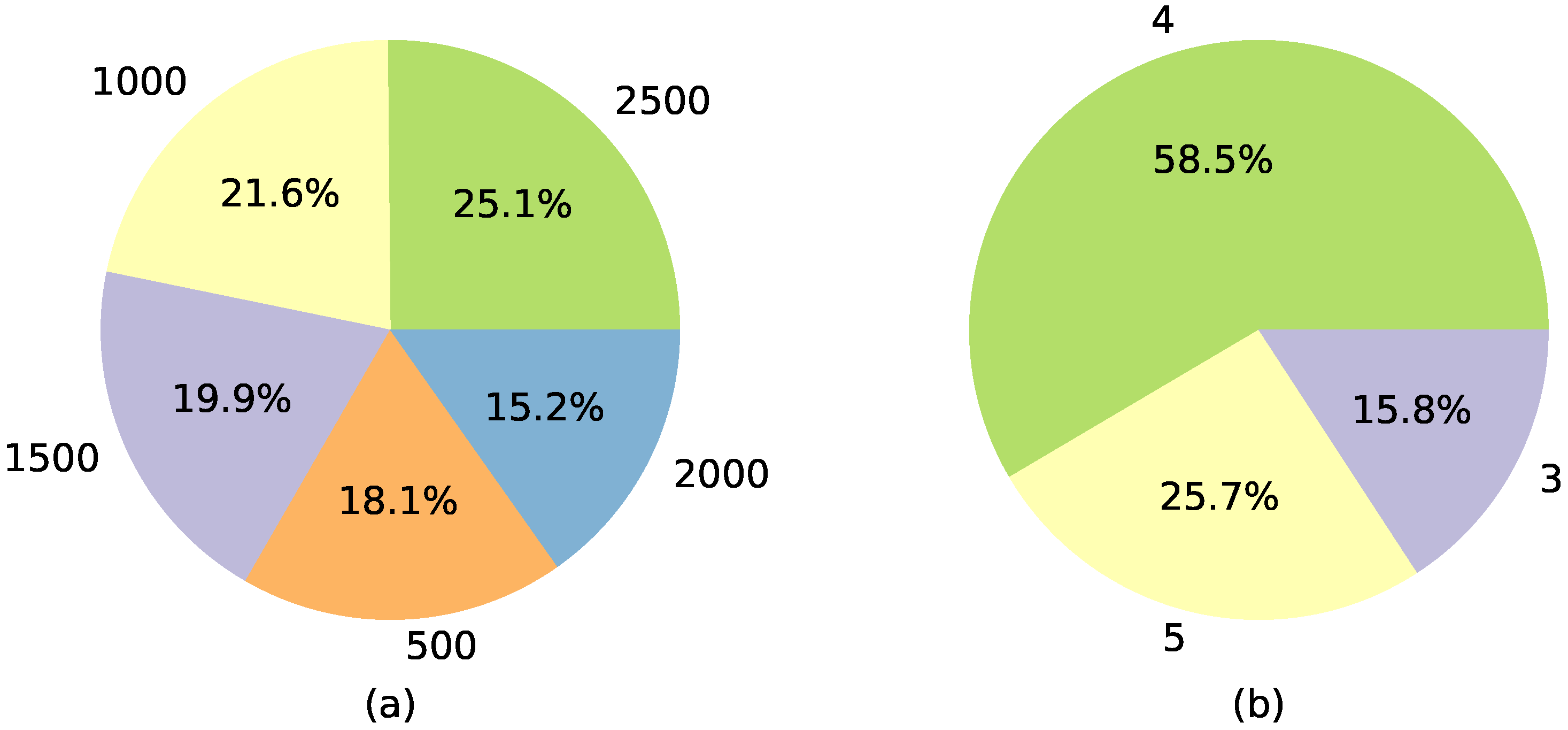
Appendix A presents a detailed statistical analysis of the whole dataset, while in this subsection, we highlight the most important insights. The left-hand-side graph in Figure 2 shows the breakdown of the contestants’ cash builder results, while the right-hand-side graph indicates the distribution of the selected offer. The success in the cash builder was relatively evenly distributed across all five options, with a slight prevalence of five correct answers in the cash builder (EUR 2500). A significant portion of the contestants (58.5%) opted to compete against four chasers, while none has ever selected to compete against two.
We noticed that as the age group increases, the percentage of contestants selecting the offer with four chasers rises, while the number of those selecting the offer with five chasers decreases. The only age group that did not choose to face four chasers most frequently was the second one (from ages 19 to 24), where as many as 47.6% of the contestants selected the offer with all five chasers. On average, older contestants tended to select offers with lower monetary prizes but a greater time advantage over the chasers than the younger ones did. An interesting observation is that younger contestants with lower results in the cash builder, on average, selected offers with more chasers compared to those of the older contestants with the same results.
Both men and women most often selected the offer with four chasers. Women selected the offer with three and five chasers with equal frequency (22%), whereas men tended to choose five chasers (27.3%) more often than three (13.2%). On average, women selected offers with EUR 1725 less prize money and a 2.3 s longer time advantage over the chasers than men did. An unexpected statistical finding was that the contestants who were recognized by the chasers from their previous participation on quiz shows or in local pub quizzes, on average, selected offers with fewer chasers and less prize money than those who were not, regardless of their cash builder result. Contestants from large cities, on average, selected offers with more chasers. Those from smaller cities competed for approximately EUR 1500 more prize money compared to that by those from middle-sized cities. Notably, 70% of the contestants from Pannonian Croatia selected the offer with four chasers.
Regarding the intended use of the prize money, the contestants who planned to spend their winnings on education or donations selected the offer with four chasers in 70% of the cases, while those who intended to use the money for entertainment did so in 60% of the cases.
When looking into the cash builder results, we observed that compared to the other contestants, those with the lowest scores for EUR 500 and EUR 1000 were more likely to select the offer with five chasers.
It is important to note that although all the contestants receive four offers, the offers are purely non-deterministic, i.e., the contestants usually receive different offers with respect to the amount of prize money, time allocated to the chasers, and the chasers themselves, making the prediction of their choice a more complex challenge than it might have initially seemed. We observed that the offers in the first season were not only significantly more generous in terms of the prize money but also more challenging regarding the amount of time allocated to the chasers. Although the contestant’s risk–reward preferences influence the selected offer, predicting the game’s outcome depends on a broader range of factors. These include not only the contestant’s profile but also the current psychological state of both the contestant and the chasers, such as stage fright or lack of concentration, which are, in this context, impossible to quantify and include in the dataset.
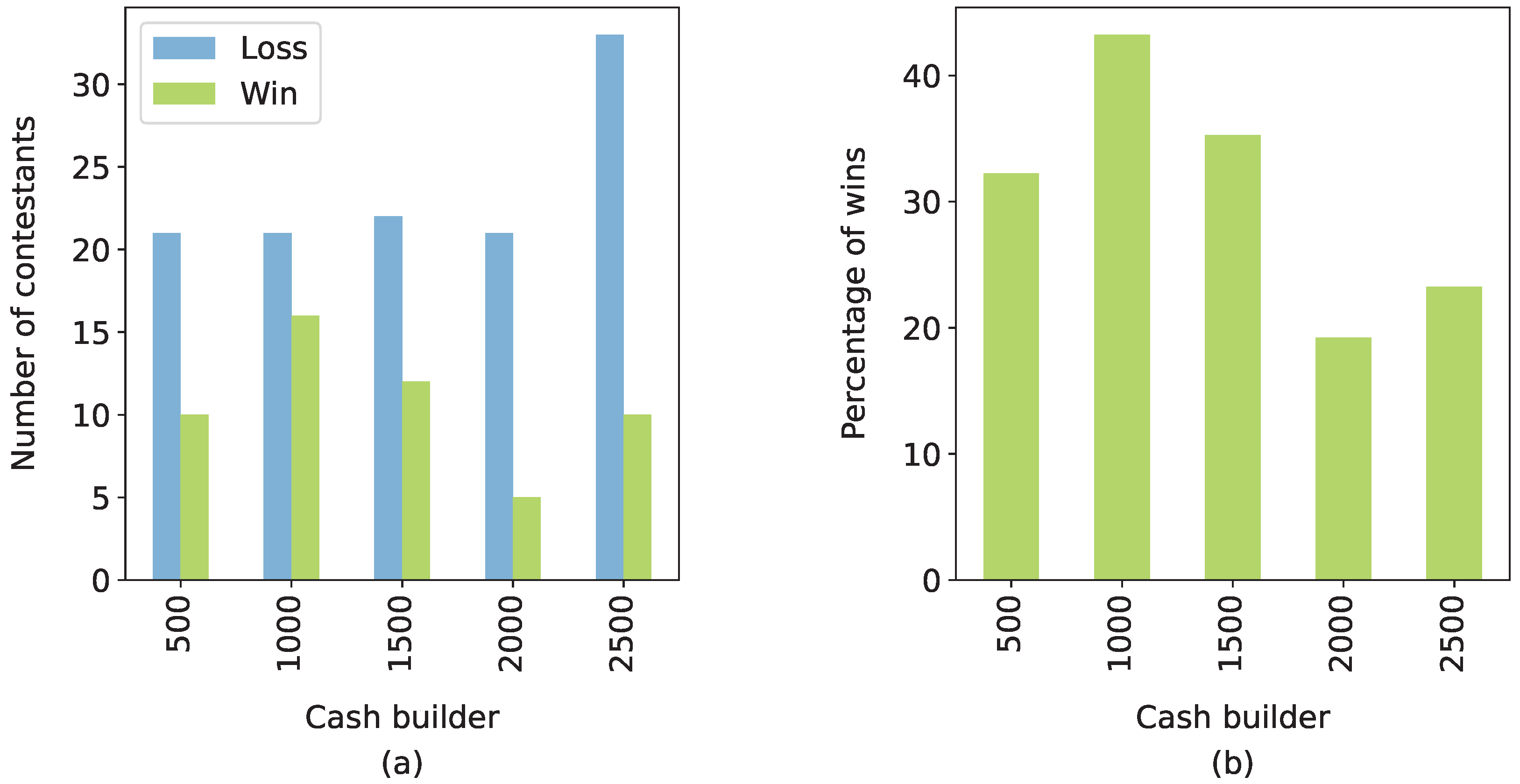
Only 31% of the contestants managed to win the prize money by beating the chasers in the second phase of the game. The most successful age group was the fourth one (from ages 35 to 44), where 42% of the contestants were victorious, while the least successful was the sixth (from ages 55 to 64) with only 10% of the victories. Regarding gender, both men and women were equally successful in about 31% of the games. Their highest winning rate was after earning EUR 1000 in the cash builder.
Figure 3 shows the relationship between the contestants’ wins and the number of chasers who participated in the final chase. In the right-hand-side graph, it is evident that as the number of chasers increases, the percentage of winners decreases, which aligns with the game’s main premise that it is harder to beat a higher number of chasers. The same can be seen in the left-hand-side graph, as the discrepancy between losses and wins increases with the number of chasers.
An analysis of the number of victories and the results in the cash builder revealed that contestants with weaker results in the first phase of the game performed better in the second phase. Figure 4 depicts the relationship between the number of victories and the cash builder results.
The thorough analysis of the dataset’s statistics revealed various interesting patterns, which prompted us to apply artificial intelligence to investigate the interactions between different features and attempt to predict the course of the game. Despite the relatively small dataset size, we aimed to leverage all the collected information to predict both the offer that a contestant would select and their success in the second phase of the game, using various machine-learning methods.

5. In the Search for a Missing Link

This section provides an overview of the analysis approach and machine-learning methods used to predict the selected offers and games’ outcomes. In the first subsection, we briefly introduce the methods and define the evaluation metrics that were used to assess the model’s performance. Section 5.2 and Section 5.3 present the results that different methods achieved when predicting the selected offer and the game’s outcome, respectively.

5.1. Methods and Evaluation Metrics

The dataset was randomly divided into training and testing sets in an 80:20 ratio. To mitigate the impact of the class imbalance problem, which leads to the degradation of the model’s performance, in addition to training the models only on the original data, we oversampled the training part of the dataset using the SMOTE (synthetic minority oversampling technique) algorithm presented by Chawla et al. in 2002 [55]. The algorithm generates synthetic examples based on the minority class examples and their closest existing neighbors. These synthetic data can help in cases of unbalanced datasets, but they can also lead to performance deterioration. In the cases where the model trained only on the original data outperformed the one trained in the oversampled dataset, we reported only the better-performing version. In each table that presents the models’ results, the use of the SMOTE is indicated by the “+” symbol in the appropriate column; the symbol “-” was used otherwise.
To predict the selected offer and the game’s outcome, we tested various types of models, ranging from logical and probabilistic approaches to artificial neural networks, tree-based methods, and ensembles. We started with a simple linear model, such as logistic regression (LR), and a support vector machine (SVM) with a radial-basis-function kernel (RBF). Next, we tested the performance of the k-nearest-neighbor model (kNN) based on example instances and both the Gaussian (GNB) and multinomial (MNB) naive Bayes probabilistic classifiers. In the next step, we investigated the performances of neural networks and decision-tree (DT) models. In each of the observed cases, we tested diverse feedforward neural network architectures and reported the best-performing one in each scenario. We used the Adam optimizer and the cross-entropy loss function (categorical for the selected offer prediction and binary for outcome predictions). For decision-tree building, we used the CART algorithm [56], first presented in 1984, which splits the tree based on the Gini impurity. To reduce the tree’s complexity and improve the model’s generalization abilities, we used cost–complexity pruning.
Moreover, we tested several ensemble methods to evaluate the performances of different model combinations. In addition to using a voting classifier with independently trained models, we also tested a random forest (RF) and extreme gradient boosting (XGBoost). Although all the mentioned methods were tested in all the observed scenarios, only the results of the best-performing models are presented in the following two subsections.
For the hyperparameter optimization, we used k-fold cross-validation with 10 folds in the training set, with the F1-score as the metric. In the case of neural networks, we used a different approach. This is the only case where we split the original dataset into three sets in a 70:15:15 ratio. The first 70% of the dataset was used for network training, while the next 15% was used for the model validation and selection of the optimal parameters. The last 15% was used for the final model evaluation. The pseudocodes for training neural networks and other models are presented in Appendix B.1 and Appendix B.2, respectively.
To evaluate the models’ performances, we used several standard evaluation metrics. In addition to extracting the confusion matrices, we also calculated the accuracy, precision, recall, and F1-score of each model. Because of the significant class imbalance for both the selected offer and outcome predictions, we used the weighted averaging of the selected metrics. The models’ performances were compared according to the achieved F1-scores. The best-performing model, according to the F1-score, is highlighted in bold in the result tables (Table 9, Table 10, Table 11, Table 12, Table 13, Table 14, Table 15, Table 16 and Table 17) in the following subsections.
To understand the models’ reasoning, we used SHAP (Shapley additive explanations) values [57], which reveal how features influenced the models’ outputs. We applied SHAP to all the methods except for the voting classifier, as it combines several individual models that use different strategies and features’ importances.

5.2. Selected Offer Predictions

The first goal of this research was to successfully predict which offer the contestant would select. Only offers with three, four, or five chasers were considered, as offers with two chasers have, so far, never been selected. The analysis was conducted in three scenarios, as presented in Table 9, Table 10 and Table 11. In the first scenario (Section 5.2.1), the models predicted the selected offer based solely on the contestant’s profile. In the second scenario (Section 5.2.2), in addition to the contestant’s profile, we also considered the result in the cash builder. In the last scenario (Section 5.2.3), we used only a subset of the contestant’s profile information. In this case, the selected offer was predicted based solely on the contestant’s gender, age group, hometown size, and NUTS 2 region. This case was considered because this was the only information that was fully available for each of the contestants without any missing values. The scenario with all the offers, including the prize money, time allocated to the chasers, and their order of appearance in the offers, was also considered but was not reported, as the results were not conclusive enough to warrant further analysis. A condensed table of features for all the analyzed scenarios is available in Table A1 in Appendix C.

5.2.1. Scenario #1: Contestant’s Profile

Table 9 shows different models’ performances for predicting the offer a contestant will select solely based on their profile. The models with the best performances were the kNN model ( k = 1 , p = 1 ) and the voting classifier (soft voting), which consisted of three independent classifiers: (1) a kNN model ( k = 1 , p = 1 ), (2) XGBoost (four estimators, l r = 0.5 ), and (3) a GNB classifier. Regarding the GNB classifier, we noticed a decay in the performance of as high as 40% when using SMOTE oversampling. For the reported XGBoost result, we used the same parameters as those used when it was included in the voting classifier. In contrast to the other reported methods, its result, presented in Table 9, was obtained without the use of oversampling. The neural network architecture ( b a t c h s i z e = 64 , 72 epochs) consisted of five dense layers with sixty-four, thirty-two, sixteen, eight, or three nodes. Each node in the hidden layers used the ReLU activation function, and the output node used softmax. After each hidden dense layer, we performed batch normalization and dropout, with rates of 0.05 after the first two layers and 0.01 after the third and fourth.
In this case, we notice that simpler models, such as kNN or GNB, outperformed complex methods, like XGBoost or neural networks. Although the kNN and voting classifier models reached the same performance level, the kNN model is preferred because of its simplicity and interoperability. Despite a high number of features, which make it difficult to visualize, it is intuitive to understand the model’s decision, as it classifies the example in the same class as its nearest neighbors. Additionally, the kNN method is suitable for applying SHAP to gain a deeper insight into the model’s decisions.
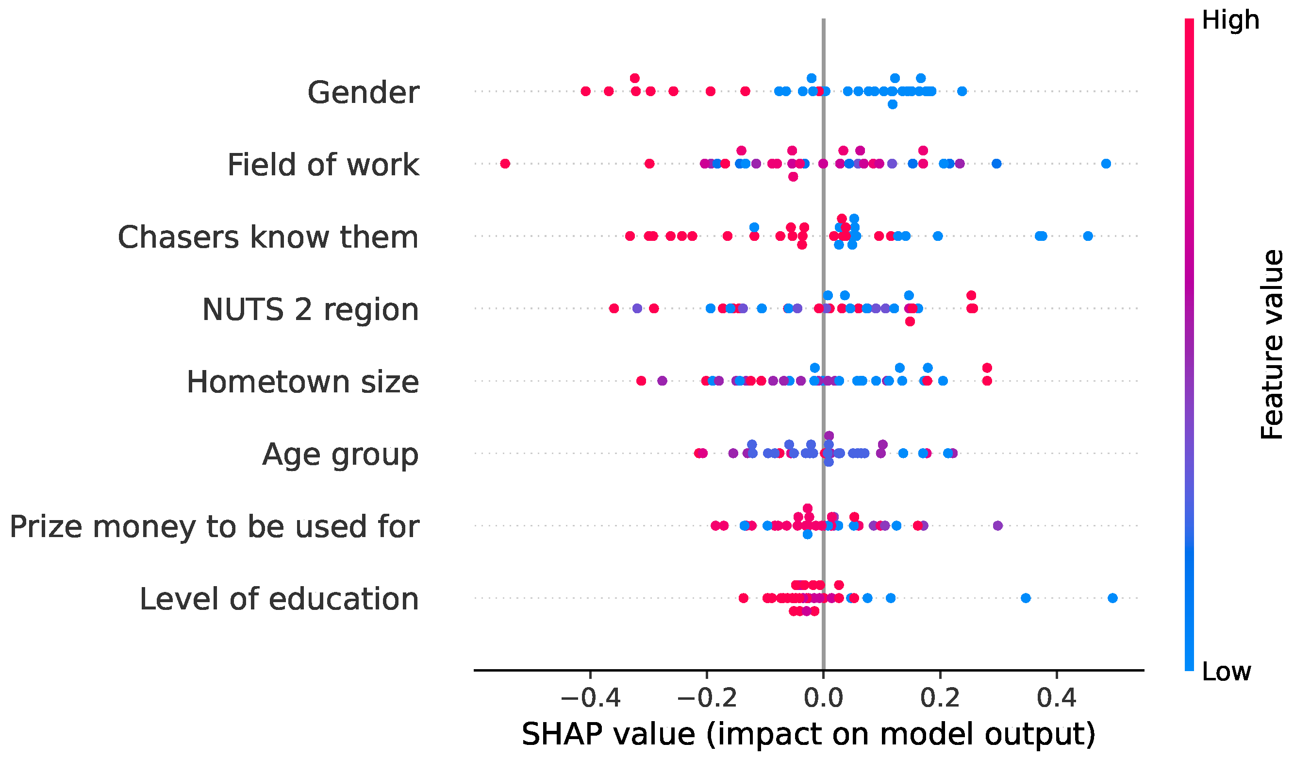
Almost all the models used in this scenario recognized the field of work and gender as the most important features. These were followed by the contestant’s age group and whether the chasers recognized them from other quizzes. The least important features were the level of education and the intended use of the prize money. In the neural network and XGBoost, the hometown size also had a minor influence on the models’ decisions, but as seen in Table 9, these models had the lowest performance metrics among the reported ones. In the GNB classifier and XGBoost, the NUTS 2 region had a weak influence, but in the kNN and neural network models, its importance was higher. In Figure 5, we present the features’ impacts for the reported kNN method. As seen in the graph, a higher value for gender led to a decrease in the model’s output, while not knowing the chasers beforehand had the opposite effect. A low age-group, lower level of education, and small hometown size also increased the model’s output, meaning that these features favor the selection of the offers with more chasers.

5.2.2. Scenario #2: Contestant’s Profile and Cash Builder Result

In Table 10, we present the results when predicting the selected offer not only based on the contestant’s profile but also taking into account their result in the cash builder. The best-performing models were similar to the ones in the previous case, including their optimal parameters (the kNN model, GNB classifier, voting classifier, and XGBoost). The only difference in the models’ parameters was the number of estimators in the XGBoost method, which was, in this case, 16. It was applied to both the individual XGBoost and the XGBoost within the voting classifier. We noticed degradations in the performances of all the models, especially the that of the kNN.
Despite the models’ lower performances in this scenario, we also performed feature analysis. Again, all the models agreed on the high importance of the field of work. The kNN model considered the cash builder result and NUTS 2 region as the most influential features, and the level of education as the least influential feature. Regarding the GNB classifier, alongside the field of work, the gender, cash builder result, and whether the chasers recognized the contestant had the strongest influences on the model’s output. The features’ influences were similar to those in the previous scenario, with the addition of the cash builder result, which lower values led to higher model outputs, pushing the model’s decision to offers with more chasers. Although the cash builder result had a strong influence on the models’ predictions in this scenario, the models’ degraded performances suggest that this feature may have misled the models in their decision making. This could indicate that the contestants might be coming to the show with a predefined choice, without considering the particular onsite offers.

5.2.3. Scenario #3: Contestant’s Partial Profile

Table 11 depicts the models’ performances for the third case, where we considered the prediction of the selected offer based on a subset of the information about a contestant (i.e., a partial profile). As there was a high number of missing values, we tried to train the models to predict what a contestant would select based on only the information that was fully available for each contestant. The performances of the GNB and neural network methods dropped by 17% and 7% percent, respectively, but reducing the number of features led to improved results for several of the other tested models. Several models achieved performance metrics over 70%, but the voting classifier (soft voting) again took the lead. Even though the voting classifier, consisting of three models, also surpassed 70%, the classifier consisting of five models outperformed all the other tested models in all the metrics. The models within it were (1) a kNN model ( k = 5 , p = 1 ), (2) an MNB classifier, (3) an SVM ( C = 10 , g a m m a = 1 ), (4) an RF classifier (127 estimators), and (5) a DT that was not pruned. For the kNN model, we used the same parameters as those in the voting classifier. Figure 6 visualizes the pruned DT ( c c p _ a l p h a = 0.0068 ) in this scenario. Although the DT without pruning performed slightly better, the tree was too complex to present the tree’s structure in the paper.
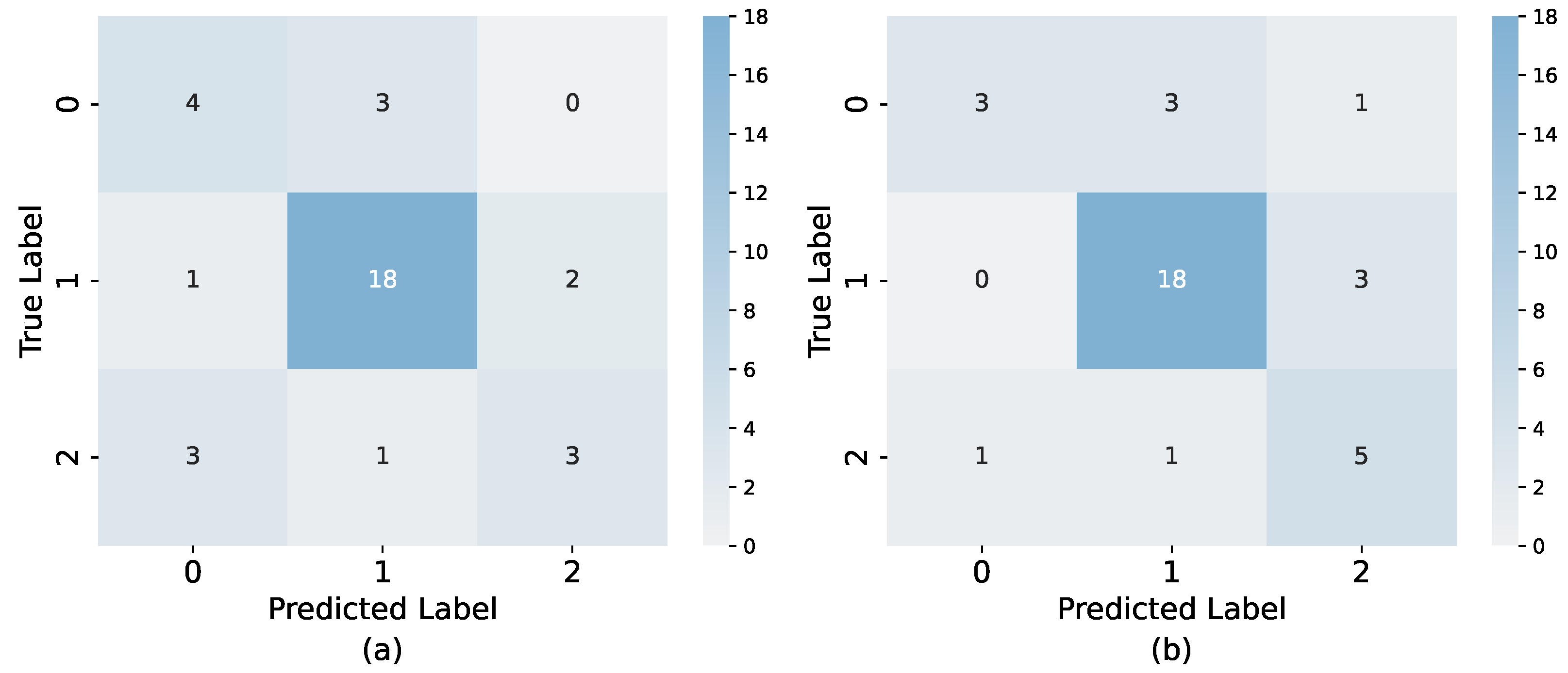
Figure 7 shows the confusion matrices for the best-performing model (voting classifier) and the model visualized in Figure 6 (pruned DT). Both models accurately recognized the contestants who selected the offer with four chasers, each misclassifying only three instances. Regarding the other classes, both models frequently predicted that a contestant would select the offer with four chasers when they had actually selected the offer with three. In cases where the true selected offer was the one with five chasers, the voting classifier performed better and misclassified only two instances. On the contrary, in such cases, the pruned DT often predicted the selection of only three chasers.
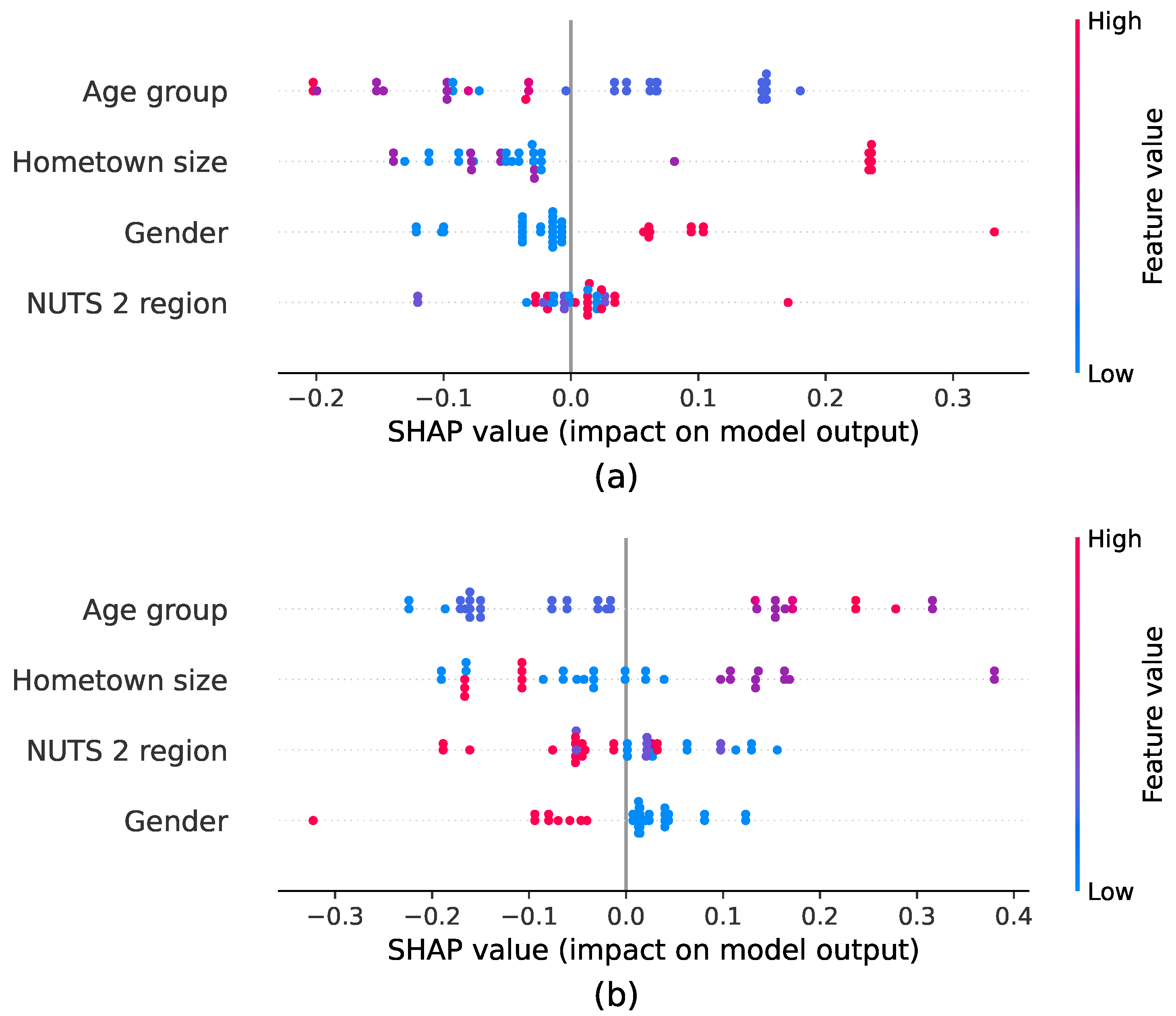
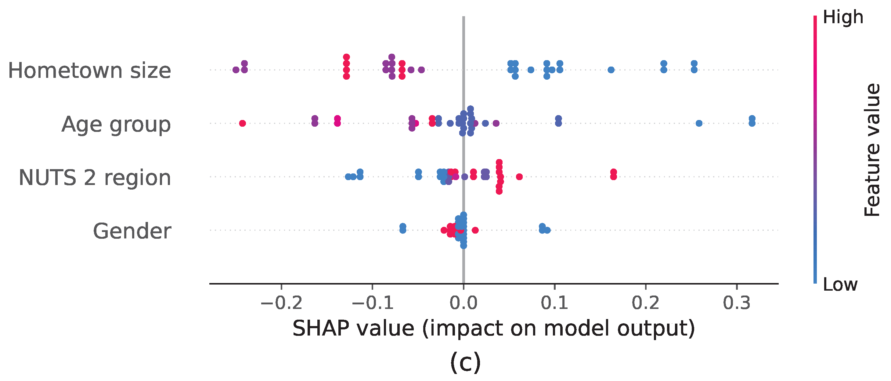
In this scenario, all the models except for XGBoost highlighted the hometown size as the most important feature and gender as the least important. In the XGBoost model, the situation was reversed, gender was the most important feature, while the hometown size had the least influence. Figure 8 presents the features’ impacts on the previously visualized pruned DT model’s output for each one of the classes. As visible in the figure, high values for the hometown size and gender tended to push the model to predict that the contestant would choose the offer with three chasers. A high value for the age group, a low value for the gender, and a middle value for the hometown size pushed the model toward predicting the offer with four chasers, while low values for the hometown size and age group and a high value for the NUTS 2 region pushed it toward the five-chaser offer.

5.2.4. Discussion on Selected Offer Predictions

We note that in all three scenarios, the voting classifier took the lead as the best-performing model. Bearing in mind a significant class imbalance, a number of missing values, and the fact that this was a multiclass classification problem, the accuracy score of 74.3%, precision of 75.2%, recall of 74.3%, and F1-score of 73.6%, which the voting classifier achieved, can be considered as successful. Only in the first case did the kNN method manage to match its performance. The other individually tested methods did perform relatively well but were far more successful when combined. We have shown that only a small subset of the information about a contestant was enough to predict the selected offer. Additional information about the contestants and the cash builder result introduced too much noise to the models, which resulted in the degradation of the performance. To substantiate this claim, we also tested the prediction using the data for the particular offers (prize money and time advantage). As expected, the models’ performances dropped even more, leaving all the performance metrics below 60%. Information about a contestant’s gender, age group, NUTS 2 region, and hometown size has proven to be optimal for determining the number of chasers a contestant would select to face. We attempted to extract a set of simple rules from the tree-based methods, but the trees were overly complex, and the test dataset was too small to confidently assert the validity of any particular rule. Given the small size of the test set and the large size of the tree, each leaf contained only a few samples from the test data.
Although we were unable to perform feature analysis for the best-performing model, we did so for all the other models. In the first two reported scenarios, the field of work was treated as one of the most prominent features by a number of the models. In the first scenario, it was accompanied by the contestant’s gender, followed by their age group, and whether the chasers recognized them. The best model after the voting classifier, in the second scenario, was the GNB classifier, which also recognized the gender, cash builder result, and whether the chasers recognized the contestant as important features. In the last, and the best-performing, scenario, where we used only a subset of the contestant’s profile information, the hometown size was highlighted as the most important and gender as the least important feature by four different models. The models’ output was pushed toward higher-value offers by lower gender and age-group values, smaller hometown sizes, lower levels of education, higher NUTS 2 region values, and if the chasers did not recognize the contestants. Higher values for the field of work, gender, level of education, and whether the contestant was recognized by the chasers had the opposite impact, pushing the models’ output toward the offers with a lower number of chasers. In the only scenario in which we use the cash builder result, we can notice that its lower values contributed positively to the model’s output, shifting the predictions to classes with a higher number of chasers. However, this approach resulted in overall declines in the models’ performances.

5.3. Outcome Predictions

The second problem we studied was the game’s outcome prediction, which we explored in six scenarios. First, the models were trained to predict the outcome based solely on the contestant’s profile (Section 5.3.1). Then, in the second case (Section 5.3.2), we included the result achieved in the cash builder, all the received offers (prize money and time advantage), the selected offer, and which particular chasers participated in the game. In a manner similar to that for the selected offer prediction, we also considered the scenario with all the available features, including the order of the chasers. However, we decided not to report it because of its lower performance relative to those of the other scenarios. In the third case (Section 5.3.3), we considered all the features from the second scenario but without the information about the contestant’s profile. In this way, we wanted to investigate whether a contestant’s profile influences the game’s outcome. The last three cases predicted the game’s outcome based on the selected number of chasers and the cash builder result in the first case (Section 5.3.4), the selected number of chasers and time advantage in the second case (Section 5.3.5), and a combination of all three previously mentioned features (the selected number of chasers, cash builder result, and time advantage) (Section 5.3.6). As in the previous case, a condensed table of features for all the analyzed scenarios is available in Table A2 in Appendix C.

5.3.1. Scenario #1: Contestant’s Profile

Table 12 reports the models’ performances in the outcome prediction based on the contestant’s profile. All the models performed better when trained only on the original data (i.e., without the use of SMOTE oversampling). Despite that, only two models can be considered as marginally successful: the neural network and voting classifier. The neural network ( b a t c h s i z e = 16 , 107 epochs) consisted of four hidden layers, with thirty-two, thirty-two, sixteen, and eight neurons, respectively. Between the first two hidden layers, we used dropout, with a rate of 0.2. The output layer consisted of a single neuron with sigmoid as an activation function. All the other layers used a ReLU activation function. The voting classifier (hard voting) consisted of three models: (1) a GNB classifier, (2) an XGBoost classifier (65 estimators, l r = 0.1 ), and (3) and an SVM ( C = 10 , g a m m a = " scale ”).
We performed feature analysis to assess the impacts of individual features on the models’ outputs. As the performance of the neural network was significantly higher than the performances of the other models, we focused on this model for further feature analysis. The features with the greatest impacts on the models’ outputs were whether the chasers recognized the contestant, the NUTS 2 region, gender, and the intended use of the prize money. In contrast, the hometown size and field of work had the least impacts. The models’ outputs leaned toward predicting that a contestant would win when they were not recognized by the chasers, when the values for gender, age group, and level of education were lower and when the value for the NUTS 2 region was higher. In contrast, the other reported methods pushed the models toward higher outputs for higher gender values.

5.3.2. Scenario #2: Contestant’s Profile, Cash Builder Result, and Offers

In Table 13, we report the outcome prediction results based on additional data. In this case, the models also took into account the information about the received offers, the cash builder result, and the selected offer, including the chasers who participated in the second phase of the game. We can notice that in this scenario, most of the models performed better when trained on oversampled datasets. The only method that performed better without SMOTE was the kNN model ( k = 1 , p = 1 ). Adding information about the specific offers improved the performances of all the methods, regardless of their complexity. Three completely different models achieved all the performance metrics above 70%. Although the voting classifier outperformed the neural network, in this scenario, in terms of the accuracy, precision, and recall, we reported the neural network as the most successful model, as we opted to grade in accordance with the F1-score. Its architecture remained the same, but the model that generalized the best was obtained after only 19 epochs. The voting classifier (hard voting) consisted of three models: (1) a kNN model ( k = 1 , p = 2 ), (2) XGBoost (24 estimators, l r = 1.0 ), and (3) an SVM ( C = 1 , g a m m a = 1 ). The parameters for the SVM and XGBoost models were the same as those for when these models were a part of the voting classifier.
Regarding the features’ importance, the SVM and kNN models considered the participation of specific chasers in the selected offer as some of the most relevant features, especially Chasers #4 and #5. The contestant’s gender also played a significant role in the SVM model, while the field of work stood out as an important feature in the kNN model. In both models, the cash builder result and whether the chasers recognized the contestant were also important features. In the tested tree-based methods (pruned DT with c c p _ a l p h a = 0.019 , RF with 50 estimators, and XGBoost), the features of the selected offer, such as the time and prize money, were the most important. The best-performing model (the neural network) also considered the participation of Chaser #4, whether the chasers recognized the contestant, and the contestant’s gender as important features. For this model, the participation of Chaser #3 and the NUTS 2 region were also considered as important. For all the models, the participation of the Chaser #4 pushed the model’s output toward predicting that a contestant would lose the game. Intuitively, longer time and more prize money in the selected offer also had the same impact. Interestingly, the influence of the gender on the neural network was opposite to its influences on the SVM and kNN models. Although in the neural network, a higher gender value pushed the model toward a positive prediction of a contestant winning the game, in the other two models, higher values for this feature shifted the prediction toward lower values, predicting that a contestant would lose the game.

5.3.3. Scenario #3: Cash Builder Result and Offers

After looking into the features’ importances for the tree-based methods in Table 13, we decided to investigate whether it is possible to successfully predict the game’s outcome based solely on the cash builder result, all the received offers, the selected offer, and the chasers who participated in the second phase. Table 14 shows the different models’ performances after excluding the information about the contestant. We can notice that the models reacted differently to the absence of the contestant’s profile information. Both the SVM ( C = 10 , g a m m a = 1 ) and the voting classifier model underwent drops in their capabilities to predict the game’s outcome successfully. The voting classifier (soft voting) consisted of (1) a kNN model ( k = 3 , p = 3 ), (2) XGBoost (77 estimators, l r = 0.5 ), and (3) a GNB classifier. When used alone, the kNN method’s ( k = 3 , p = 1 ) F1-score slightly deteriorated, but its accuracy, precision, and recall improved by around 5%. The performances of the pruned DT (maximum tree depth = 2) and XGBoost (77 estimators, l r = 0.5 ) methods remained unchanged. The models which performance increased were the LR, RF (162 estimators), and neural network. Like in the previously considered setup, the neural network was the most successful approach, predicting the game’s outcome with an accuracy of 80.8%, a precision of 79.4%, a recall of 80.8%, and an F1-score of 79.9%. The only change in the network’s architecture from those in the previous two cases was increasing the number of nodes in the first hidden layer from 32 to 64. The network reached the optimal performance in the validation dataset after only 12 epochs.
When looking into the features’ importances, the models with higher performances, such as the neural network, pruned DT, and RF, highlighted the prize money and chasers’ time in the selected offer, alongside the participation of Chaser #4, as the most relevant features. Again, both the longer time and more prize money in the selected offer and the participation of Chaser #4 led the model toward predicting the negative outcome for the contestant. Simpler models (LR, SVM, and kNN) considered the cash builder result as one of the most important features, with lower values pushing the prediction in favor of the contestant.
These results showed that the game’s outcome was influenced more by the game-specific information than by the contestant’s profile. The cash builder result, the chasers’ time in the selected offer, and the selected number of chasers were the most relevant features for predicting the game’s outcome. Nevertheless, these features were also indirectly influenced by the contestant. First, the cash builder results reflect some information about the contestants’ quizzing abilities. Second, different contestants did not receive identical offers independently of their potentially equal performances in the cash builder. This suggests that the offers may have been tailored for a specific contestant, potentially influencing their selection.

5.3.4. Scenario #4: Selected Number of Chasers and Cash Builder Result

In the next step, we wanted to determine how well the models can predict the game’s outcome based on only two pieces of information: the selected number of chasers and the cash builder result. In this scenario, the only information that depended on the specific contestant was the result in the cash builder. The selected number of chasers depends on the contestant’s preferences but does not reveal their skill in the next phase of the game. Table 15 gives insight into the different models’ performances. A number of the models performed well despite considering only two input features. All the models except for the GNB classifier performed better when trained on the oversampled dataset. LR, the kNN model ( k = 5 , p = 1 ), the GNB classifier, the DT, the RF (91 estimators), and XGBoost (58 estimators, l r = 1.0 ) all reached F1-scores of over 65%. The voting classifier (soft voting) consisted of (1) a kNN model ( k = 5 , p = 1 ), (2) a GNB classifier, and (3) an SVM ( C = 0.1 , g a m m a = “scale”), and all its performance metrics reached over 70%. A voting classifier with five models was also tested, but the performance remained unchanged. Again, the neural network was the most successful approach, with its accuracy, recall, and F1-score over 80% and its precision slightly over 90%. The architecture was the same as those in the first two cases, where we predicted the outcome based on the contestant’s profile. The optimal performance was reached after 108 epochs.
For all the reported models except for the kNN and DT, the selected number of chasers was more important information than the cash builder result. Again, a higher selected number of chasers and a high cash builder result led the models toward a lower output, predicting that a contestant would lose the game. In the neural network, only the mid-range values for the cash builder results pushed the model’s output toward a positive prediction. In this case, lower values for this feature had the same impact as the high values, pushing the model toward predicting a negative outcome for the contestant.

5.3.5. Scenario #5: Selected Number of Chasers and Time Advantage

In the next scenario, we used the selected number of chasers and the chasers’ time in the selected offer to predict the game’s outcome. In this case, none of the input features depended on the contestant’s profile. By doing so, we wanted to examine the model’s ability to predict the game’s outcome based solely on objective, game-specific data.
As presented in Table 16, several models reached high performances. The SVM, GNB classifier, and voting classifier performed better when trained only on the original data. The rest of the models were more successful when trained in the oversampled dataset. Five models had identical accuracies, precisions, recalls, and F1-scores of 77.1%, 82.9%, 77.1%, and 72.2%, respectively. As expected, the models failed to correctly predict the game’s outcome in cases when a contestant managed to unexpectedly defeat all five chasers despite a small time advantage they had over the chasers. Several model combinations were tested for a joint voting classifier (soft voting). The best-performing combination was using (1) an SVM ( C = 10 , g a m m a = “scale”), (2) XGBoost (42 estimators, l r = 0.05 ), and (3) a kNN model ( k = 5 , p = 2 ). For both the SVM and XGBoost, we used the same parameters as those for when these models were used as a part of the voting classifier. The only model that managed to handle a part of the outliers and achieve performance metrics over 80% was the neural network. With its network architecture unchanged from those of the previous scenarios and a change in the batch size to 32, it reached the optimum performance after 105 epochs.
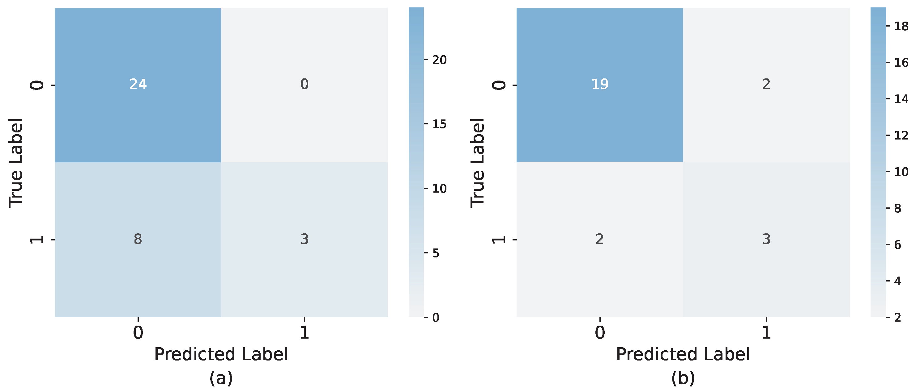
The confusion matrices for the pruned DT (visualized later in the text) and the best-performing model in this scenario are shown in Figure 9. The total number of test samples differs between the models because for the pruned DT, we used 20% of the dataset for testing, while for the neural network, 15% of the dataset was allocated for validation, leaving only 15% for testing. As seen in the left-hand-side confusion matrix, the pruned DT accurately recognized the contestants that lost the game but struggled to identify the victorious ones, often misclassifying them. On the right-hand side, it is visible that the neural network was more successful in recognizing the contestants who would win the game.
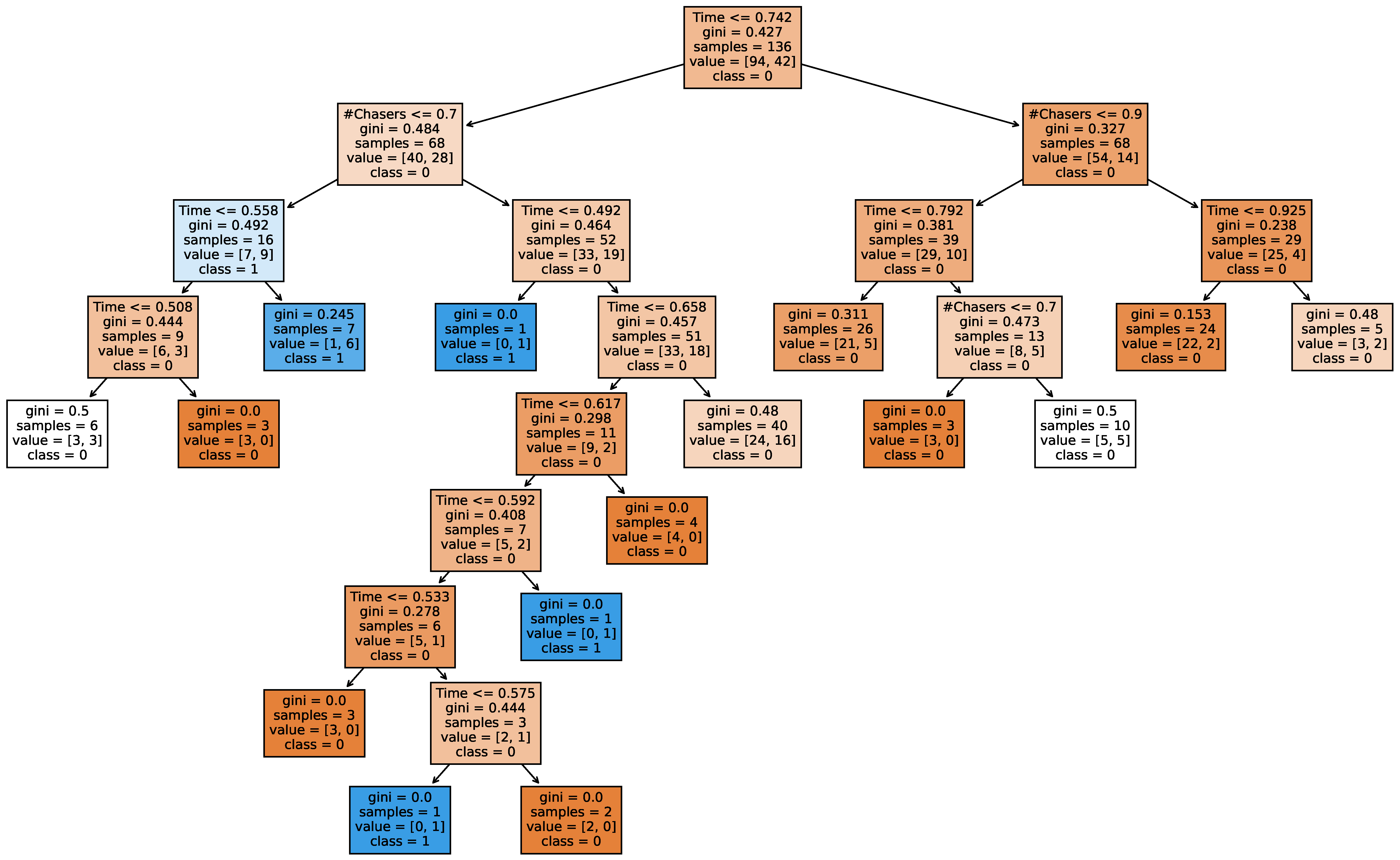
In Figure 10, we present the final pruned DT ( c c p _ a l p h a = 0.004 ) for this scenario. Although the pruned DT achieved a performance equal to those of the SVM, GNB classifier, voting classifier, and XGBoost, it stands out as the most interpretable model and the easiest to visualize among them. Its transparent tree structure clearly shows which conditions led to each decision of the model.
The pruned DT and XGBoost considered the chasers’ time in the selected offer as a more important feature than the number of chasers in the same offer, while all the other reported models favored the opposite. A low number of chasers and a short chasers’ time in the selected offer led to more optimistic outputs, pushing the models to predict that a contestant would win the game. Figure 11 shows the impact of both used features on the model’s output for the neural network presented in this scenario. We can see the stronger impact of the selected number of chasers, with high values having a negative impact on the model’s output, mid-range values moderately shifting the output toward positive predictions, and low values pushing the model toward positive predictions. For the chasers’ time in the selected offer, we can see not only a weaker impact but also higher values decreasing the model’s output and lower values increasing it.
These results indicate that it is possible to predict the game’s outcome independently of the contestants’ profiles, using only two features, with all the selected evaluation metrics above 84%.

5.3.6. Scenario #6: Selected Number of Chasers, Cash Builder Result, and Time Advantage

In the last scenario we report in this paper, we decided to combine the previous two scenarios and use the selected number of chasers, the cash builder result, and the chasers’ time in the selected offer for game’s outcome prediction. The previous two scenarios showed promising results, which led us to investigate how these three features would work when combined but without any other information.
Table 17 gives an overview of the results. As many as six different models reached an F1-score of higher than 72%, while the voting classifier and neural network exceeded an F1-score of 82%. The neural network had higher precision, but the voting classifier had higher accuracy, recall, and a slightly higher F1-score. It used three hard voting models: (1) a kNN model ( k = 1 , p = 1 ), (2) an RF (27 estimators), and (3) an MNB classifier. The same parameters were used for the independently trained and tested kNN and RF, which results are also reported in Table 17. For XGBoost, we used 73 estimators and l r = 1.0 . The neural network’s architecture remained the same as that in the previous scenario, but we used a batch size of 16 in this case. The optimal performance was reached after 104 epochs. It is important to note that all the mentioned methods (the voting classifier, kNN model, RF, and neural network), alongside the GNB classifier, had a high precision score. As can be seen in the table, pruning the DT ( c c p _ a l p h a = 0.003 ) did not lead to any performance degradation, but in contrast to the full DT, it performed better in the oversampled dataset.
In this scenario, the DT, pruned DT, and RF ranked the cash builder result as the most important feature, followed by the chasers’ time in the selected offer, and, ultimately, the selected number of chasers. The model with the highest performance after the voting classifier (the neural network) identified the selected number of chasers as the most important feature, and the cash builder result as the least important one. As in the previous scenarios, for all models except for the neural network, a higher cash builder result decreased the model’s output, while a lower one increased it. As seen in Figure 12, in the case of the neural network, mid-range values for the cash builder result pushed the model toward a positive prediction, while high and low values shifted the model toward predicting the negative outcome for the contestant, just as in scenario #4. A lower selected number of chasers increased the outputs of all the tested models. Although, in the majority of the models, a higher value for the chasers’ time in the selected offer led to a decrease in the output, in the neural network, a higher value for this feature favored the contestants by increasing the model’s output.
Observing the results, we can conclude that introducing the cash builder result to the combination of the selected number of chasers and the chasers’ time in the selected offer led to an overall improvement in the model’s results. Although the best-performing option remained the neural network that predicted the outcome based on the selected number of chasers and their time, the information about the cash builder results boosted the performance of the other tested methods. On average, the best results were obtained when using these three features.

5.3.7. Discussion on Outcome Predictions

By comparing all the analyzed cases, we noticed that the features that were not related to the contestant’s profile, but instead to the game-specific details, had a greater impact on the game’s outcome. Using only the information about the number of chasers and their assigned time, we managed to classify 84.6% of the test examples accurately. In five out of the six scenarios, the neural network stood out as the most successful predictor. The only scenario where the voting classifier outperformed the neural network was the last one, which predicted the game’s outcome according to the information about the selected number of chasers, the cash builder result, and the chasers’ time in the selected offer. Like in the previous analysis, where we considered the selected offer prediction, using too many features introduced noise to the models and decreased their successful prediction abilities. As in the previous subsection, we attempted to derive simple rules for outcome predictions using tree-based methods. However, the complexity of the trees and the small size of the test dataset hindered our ability to validate any rules reliably. Given the limited number of test samples and the large size of the tree, each terminal node contained only a low number of test cases, making it difficult to draw conclusions confidently.
Given that the models used in the last three scenarios, which combine the selected number of chasers, the cash builder result, and the chasers’ time in the selected offer, reached the best performance, we can consider these features as the most relevant ones. In most scenarios and models, their higher values pushed the model’s output to predict the defeat of the contestant, while their lower values did the opposite. The only exception was the neural network, where only mid-range values for the cash builder result favored the prediction of the contestant’s victory. Also, in scenario #5, a higher value for the chasers’ time in the selected offer increased the neural network’s output. The contestant’s gender and whether the chasers recognized them were the most influential features of the contestant’s profiles. Although the contestant’s gender had different impacts across the different models, in the neural networks that had the best performance in both scenarios where the contestant’s profile was taken into account, a higher value for the gender tended to push the model’s output toward higher values. Not being recognized by the chasers also led the models toward predicting a positive outcome. A number of the methods treated the participation of Chaser #4 as one of the most important features, pushing the model’s output toward predicting the negative output if that chaser was present.

6. Conclusions

In this section, we conclude the paper with a brief overview of the results, a discussion of this study’s limitations, and the provision of future work perspectives.

6.1. Result Overview

In this paper, we presented an in-depth analysis of the Beat the Chasers TV game show. Initially, we described the game with its rules and propositions, followed by the first contribution of the paper: the dataset obtained by extracting data from publicly aired episodes of the first two seasons of the Croatian version of the show. The dataset was studied from the perspectives of descriptive and semantic statistical analyses. As the main contribution of the paper, we applied several machine-learning methods to the data in two separate contexts.
First, we aimed to identify which offer a contestant would select based on the following information:
1.
The contestant’s profile;
2.
The contestant’s profile paired with the cash builder result;
3.
The contestant’s partial profile (gender, age group, hometown, and NUTS 2 region).
Predicting the contestant’s choice was a challenging task not only because of the different contestant profiles but also because of the variety of offers. Despite the same performance in the cash builder, the contestants received different offers in terms of the amount of the prize money, the amount of time allocated to the chasers, and the chaser lineup for specific offers. Table 18 sums up the results of all the models for all the scenarios described in Section 5.2, including the model parameters and the use of SMOTE oversampling. The voting classifier yielded the best results in all three scenarios, with the contestant’s partial profile (third scenario) achieving an F1-score as high as 73.6%. Only in the first scenario did the k-nearest-neighbor model manage to match the performance of the voting classifier. By looking at Table 18, we can notice that all the models reached their best performances in the third scenario, where we only used the features that were explicitly extracted from the show and that did not have any missing values. Regarding the first two scenarios, the results showed that adding the cash builder result degraded the performances of all the tested models, which might lead to a suspicion that the contestants’ cash builder results do not influence their choices and that the contestants usually come to the show with a forethought about the offer they would select.
To assess the impacts of individual features on the models’ outputs, we utilized SHAP values for all the applicable models (with the exception of the voting classifier). In the first two reported scenarios, we identified the field of work as the most impactful feature. The contestants’ gender and whether the chasers recognized them also played significant roles in both scenarios. The second scenario included the cash builder result and the particular offers in the feature set. It highlighted the importance of the cash builder result, with lower values pushing the model’s output to higher values (i.e., the offers with more chasers). However, as previously mentioned, this approach degraded the models’ performances. In the final scenario, with the best overall performance, the hometown size was the most impactful and gender was the least impactful feature in most of the models. Lower values for the gender, age group, hometown size, and education level but higher values for the NUTS 2 region and chasers not recognizing the contestant tended to shift the model’s predictions toward higher-value offers. In contrast, higher values for the field of work, gender, education level, and whether the chasers recognized the contestant pushed predictions toward offers involving fewer chasers.
Regarding the binary classification problem of outcome predictions, we focused on several combinations of features with the goal of maximizing the prediction abilities of the used models. The feature combinations (scenarios) that we took under deeper consideration were as follows:
1.
The contestant’s profile;
2.
The contestant’s profile, the cash builder result, all the offers, and specific chasers within the selected offer;
3.
The cash builder result, all the offers, and specific chasers within the selected offer;
4.
The selected number of chasers and the cash builder result;
5.
The selected number of chasers and the chasers’ time in the selected offer;
6.
The selected number of chasers, the cash builder result, and the chasers’ time in the selected offer.
The results, parameters, and use of SMOTE in all the models and scenarios are summarized in Table 19. In the majority of the scenarios, the neural network yielded the best result, reaching a prediction accuracy of as high as 84.6% for the combination of the number of chasers and the chasers’ time in the selected offer (5). On average, the best performance was reached when also including the cash builder result (6).
We also utilized SHAP values to interpret the models’ decisions in the outcome prediction task. As the best-performing models were the ones in the last three scenarios, which used only the selected number of chasers, the cash builder result, and the chasers’ time in the selected offer, we emphasize these features as the most impactful ones. In most cases, higher values for these features led the models to predict that the contestant would lose the game, while lower values pushed the models’ outputs to decide the opposite. The best-performing model in almost all the cases, the neural network, was the only model where the mid-range value for the cash builder result pushed the model’s output toward predicting that a contestant would win, while its lower values shifted the model’s prediction toward a negative outcome for the contestant. Regarding the other features, the participation of Chaser #4, the contestant’s gender, and whether the chasers recognized the contestant were the most impactful features. In the best-performing model (the neural network), a higher value for gender and not being recognized by the chasers led the model’s outputs to predict that a contestant would win the game. The participation of Chaser #4 was also considered as important by several models, with their participation shifting the model’s output to lower values.
Although the voting classifier stood out as the best-performing model in several scenarios, the other models are generally preferred in cases where they achieve a similar performance level. By applying SHAP to these models, we were able to clarify the decision process and justify the final classification. In contrast, the voting classifier lacked clear reasoning, making its decisions challenging to explain. In the best-performing scenarios, for both the selected offer and the outcome prediction, we presented a pruned decision tree, which visualized the decision process (Figure 6 and Figure 10), making the model classification interpretable.
These results have shown that the selected offer depended more on the contestant’s profile rather than their cash builder result or particular offers. In contrast, the game’s outcome was more dependent on the game-specific features, like the number of chasers, the cash builder result, and the amount of time the chasers received in the second phase of the game, rather than the contestant’s profile. These results can help both the show’s producers and the contestants. The show’s producers can use the information about a contestant for personalized offer tailoring, making the show more suspenseful. The contestants can benefit from this research by predicting their performance in the second phase of the game, which would help them in selecting the optimal offer.
Although this study focuses exclusively on the Croatian version of Beat the Chasers, the question of generalizability to other versions of the show, or even other TV quiz shows, arises naturally. We tend to be of the opinion that cultural and socioeconomic factors may influence contestants’ behaviors. For instance, one might hypothesize that contestants from less affluent regions are more motivated by potential financial gain, while those from wealthier areas may primarily participate for fun or experience. However, such interpretations are purely speculative and cannot be confirmed or refuted within the scope of this study.
In this study, we do not specifically address cultural factors, and although we acknowledge that contestants’ behaviors may, indeed, be culturally specific, our current data and methodology do not allow for definitive conclusions. The features and methods used in our models are appropriate for the Croatian context but may not transfer directly to other countries without model retraining and feature reselection, as different cultural or structural dynamics could render other variables as more relevant. For example, Croatia is highly centralized around its capital, Zagreb, with relatively few large urban centers. This centralization may influence contestants’ representation and behaviors in ways that differ significantly from those in countries with more evenly distributed populations and multiple major cities. Therefore, although some insights may be broadly applicable, we refrain from asserting that our conclusions hold universally.

6.2. Limitations

It is important to mention that even though the dataset provided as a part of this paper can be considered as being relatively wide feature-wise, it is still far from complete. A large amount of data that could significantly influence the prediction models is not publicly available. For starters, we lack the data from the contestants’ application forms, in which the contestants explicitly provide information on their personal traits. Additionally, we do not have any information describing a contestant’s quizzing skill level, which could be a key factor for accurate predictions. To compensate for this, we used data on the cash builder result and included whether the chasers recognized the contestant, assuming they were more familiar with skilled individuals. Furthermore, for both the selected offer prediction and the outcome prediction, deriving simple rules using tree-based methods was not feasible. This was primarily because of the complexity of the generated trees and, more importantly, the relatively small size of our dataset, which limited the rule extraction.
Although the total number of samples in the dataset is relatively low for machine-learning tasks, the dataset provided sufficient information for the models to perform well. To prevent overfitting during the model training, we used cross-validation for the neural networks and pruning of the decision trees. The built-in bootstrapping mechanism helped to reduce overfitting in random forests.
Although some of the limitations presented in this subsection could conceivably be mitigated by increasing the dataset size, we are currently unable to do so. For the Croatian version of the show, all the available episodes that are a part of complete seasons were included in the analysis at the time of the publication of this paper. In contrast, international versions of the show are not directly applicable to this study for several reasons. Primarily, we are not able to make categorical claims about the influences of cultural differences on the findings of this study, as such differences may, indeed, play different roles. In addition, other versions of the show can differ significantly in terms of the rules and propositions of the game. For example, the British version features different chasers across seasons and even varies in the number of chasers (some seasons include six). The German version features seven chasers; the Australian version, four chasers; and the Finnish version, only three chasers. International versions with five chasers might be applicable to our research (e.g., the Czech or Dutch versions), but it still remains unclear whether the offers in various versions of the show are commensurate with those in the Croatian version in terms of the prize money and chasers’ time, and whether contestants’ strategies or preferences are influenced by cultural factors.
Many contestants also mentioned the amount of money they would be satisfied with. This information could play a significant role in the offer-tailoring process but was excluded because of a high number of missing values. Furthermore, some of the age groups, educational levels, or fields of work lack higher representability. Although we were able to draw valid conclusions from the dataset used in this research, one could easily claim that the set itself contains a relatively low number of samples (171) for further and more advanced analyses. Despite these limitations, the dataset serves as a strong starting point for further research, providing valuable insights and establishing a foundation for future studies with more comprehensive data.
Another factor that could play a key role in the further improvement of the models’ performances is the psychological state of the contestants. People react to stress differently. Potential anxiety, stage fright, or an adrenaline rush could lead to cognitive blocks or impulsive reactions that could result in poor performance. Unfortunately, this information is impossible to obtain accurately by observing the contestants. To gather such information, the contestants should undergo an appropriate psychodiagnostic assessment or wear a device, such as a smartwatch or a fitness tracker, that can assess the stress level by measuring the heart rate variability, pulse, respiratory rate, and activity.
We can also freely assume that the production team has a predefined budget, which could induce the intra-show dependency in a way that the offers depend on the success of the other contestants in the quiz. On the other hand, we cannot exclude cross-show dependency because TV productions usually share a budget at the level of the entertainment program, which could mean that the success of other TV quiz shows produced by the same broadcasting company could influence the offers in this show.

6.3. Future Work

There are several directions for possible future work. The first step is to update the dataset with the information on the contestants and the offers from the upcoming seasons. These data could be used for further model testing or retraining in a larger dataset. Different neural network architectures could also be investigated, as the tested architectures were fairly simple. Future work could involve incorporating other international versions of the quiz rather than limiting the analysis to the Croatian version.
A major potential extension of this research would involve examining the human behavioral factors of the contestants, including not only decision making but also other psychological factors, such as stage pressure, performance anxiety, and stage fright, as well as individual personality traits. Conducting such a study would require involving experts in psychology to ensure appropriate the methodology and result interpretation.
Beyond the immediate context of TV quiz shows, the methods and paradigms presented in this study could be used in other contexts and applications. Machine-learning models capable of predicting users’ decisions based on users’ profiles and in the absence of more detailed contextual data could influence the development of personalized recommendation systems. Similarly, the approach presented in this study could be extended to simulate users’ behaviors in gamified environments, enabling tailored user engagement strategies and more adaptive game designs. On the other hand, the ability to predict decisions and their outcomes from a limited set of inputs might also influence predictive marketing, where the anticipation of users’ choices can offer better customer targeting. The aforementioned application highlights the value of data-driven behavioral modeling within the contexts in which the decisions are influenced by personal traits.
Another possible research direction we aim to take is to investigate the offers more deeply. A quantitative metric of an individual offer remains an open question. By validly defining such a metric, claims regarding the fairness of the offers could be made. After collecting a sufficiently large dataset, another option could be the prediction of the specific offers that the production staff would propose to a particular contestant according to their profile and cash builder result. Another possible research direction is the prediction of the optimal offer, which balances the winning probability and the prize money with risks, such as the number of chasers and their allocated time. This way, each contestant could be advised on which offer to select to beat the chasers.
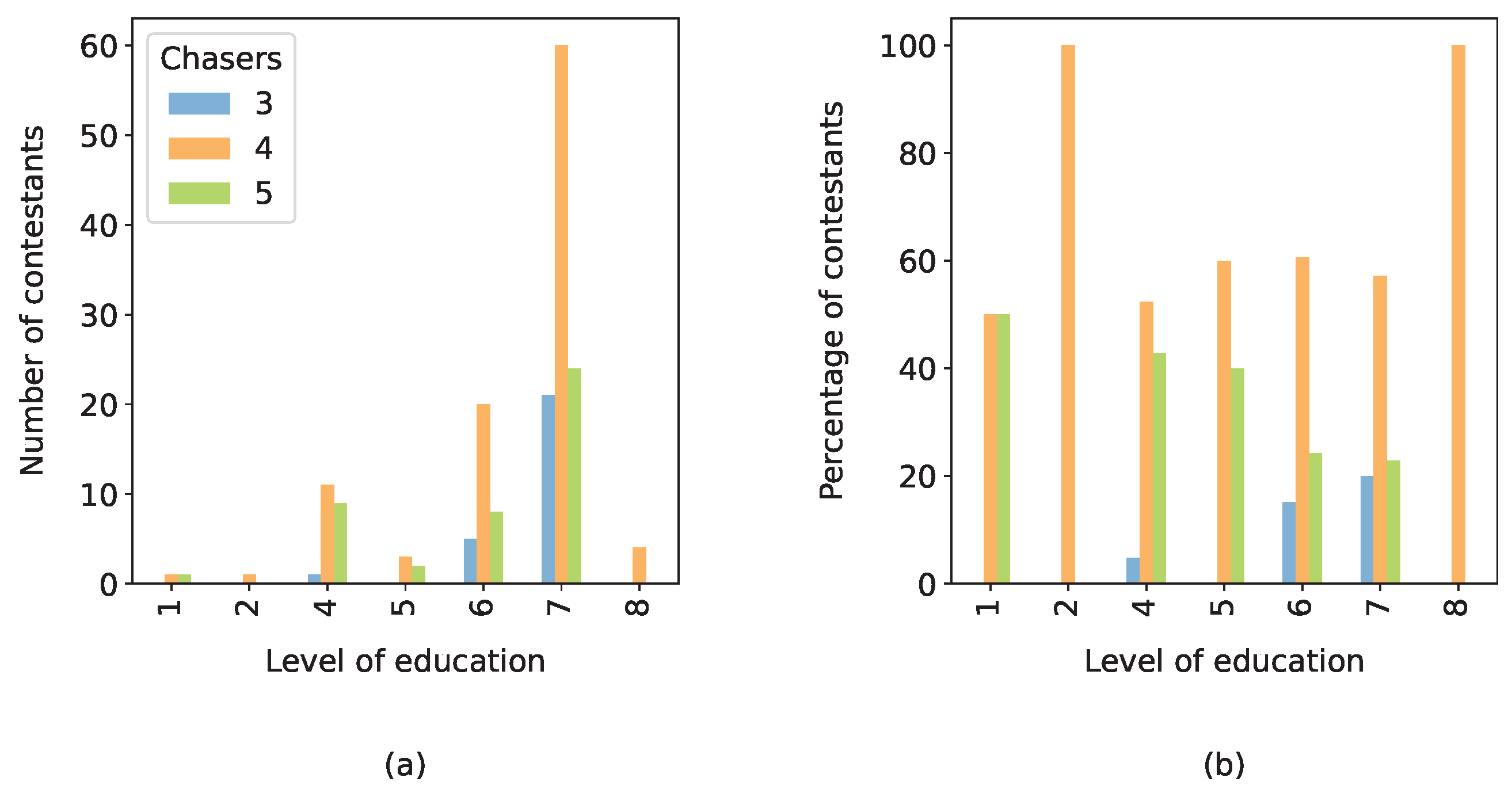
Author Contributions

Conceptualization, H.I. and B.P.; methodology, H.I., B.P. and A.J.; software, H.I.; validation, H.I., J.K. and A.J.; formal analysis, H.I. and A.J.; investigation, H.I. and B.P.; resources, H.I., B.P. and J.K.; data curation, H.I. and B.P.; writing—original draft preparation, H.I. and B.P.; writing—review and editing, H.I., B.P., J.K. and A.J.; visualization, H.I.; supervision, A.J.; project administration, J.K. and A.J. All authors have read and agreed to the published version of the manuscript.

Funding

This research received no external funding. The authors conducted the research as a part of their employment at the University of Zagreb Faculty of Electrical Engineering and Computing.

Institutional Review Board Statement

This study did not require ethical approval because of the nature of the collected data. A TV quiz is a form of a public performance, meaning that all the participants have already consented to the public disclosure of their information by participating. Our research merely collected and recorded already publicly broadcast information. Furthermore, all the data were anonymized (i.e., names were removed and ages were reported as age groups rather than concrete numbers), shuffled, and processed in an aggregated and statistical manner. This approach ensures the privacy and anonymity of the participants. Both Convention 108 of the Council of Europe and the GDPR state that personal data are no longer considered as personal if they have been rendered as anonymous.

Informed Consent Statement

Not applicable.

Data Availability Statement

All the data described in the paper and required to replicate the study findings (including the reported means) are openly available at Mendeley Data: http://doi.org/10.17632/b2zpfbhrmb.1.

Conflicts of Interest

The authors declare no conflicts of interest.

Abbreviations

The following abbreviations are used in this manuscript:
SMOTEsynthetic minority-oversampling technique
LRlogistic regression
SVMsupport vector machine
RBFradial basis function
kNNk-nearest neighbor
GNBGaussian naive Bayes
MNBmultinomial naive Bayes
DTdecision tree
RFrandom forest
XGBoostextreme gradient boosting
SHAPShapley additive explanations
ReLUrectified linear unit
lrlearning rate

Appendix A. Factual Description of the Dataset

Only 50 contestants were women, while the rest were men. The most-represented age group was the third (from ages 25 to 34) group, accounting for 36.8% of the contestants. This was followed by the fourth (from ages 35 to 44) age group, which made up 26.3% of the contestants, while the first (up to 18 years of age) and seventh (older than 65 years of age) age groups were the least represented, with 0.6% and 1.8% of the contestants, respectively (labeled according to Table 2). A significant portion of contestants (61.4%) had completed the seventh (i.e., master’s level university study) level of education. Another 19.3% had completed the sixth (i.e., bachelor’s level university study) level of education, and 12.3% the fourth (i.e., high school diploma) level. Labels depicting the levels of education are presented in Table 3. Regarding the fields of work, the most represented were the social sciences (5) and humanities (6), followed by the technical (2) and natural (1) sciences, and then the biomedical and health (3) sciences (labeled according to Table 4). Artistic and interdisciplinary fields were represented by less than 5% of the contestants. The chasers knew about 59.6% of the contestants beforehand. Approximately 53.8% of the contestants intended to spend their winnings on leisure (3), while only 5.3% cited education or donation (4) as their primary purpose (labeled according to Table 7).
As many as 40.4% of the contestants came from the City of Zagreb (1), followed by 33.3% from Adriatic Croatia (4), and 16.4% and 9.9% from Northern (2) and Pannonian (3) Croatia, respectively. The majority of the contestants came from large cities (1), while only 14% were from smaller cities (2). The labels used are derived from Table 6 and Table 5, respectively.
Regarding the selected offer, in the sixth age group (from ages 55 to 64), as many as 70% of the contestants opted to compete against four chasers. Notably, 33.3% of the contestants from the oldest age group (≥65 years) selected three chasers, whereas only 8.9% of the contestants from the fourth group (from ages 35 to 44) made the same choice.
On average, more educated individuals tended to select offers with fewer chasers and less prize money compared to those of contestants with lower educational levels. As shown in Figure A1, the frequency of selecting the offer with three chasers increased, while that of the selection of the offer with five chasers decreased with higher educational levels, with exceptions in groups 2 and 8, which are highly underrepresented, with only one and four samples, respectively. On the left-hand-side graph in Figure A1, the dataset’s imbalance is evident because of the significant dominance of the seventh education group (master’s level university study).
Figure A1. (a) Numbers of selected offers with respect to the contestants’ levels of education; (b) percentages of selected offers with respect to the contestants’ levels of education.
Applsci 15 05722 g0a1
Contestants from interdisciplinary fields, on average, selected offers with fewer chasers compared to other contestants, while those from biomedical and health sciences, as well as technical sciences, tended to select offers with more chasers. Those from biotechnological and artistic fields opted for offers with less time allocated to the chasers.
Contestants from Northern Croatia, on average, selected the offers with the fewest number of chasers, whereas those from Adriatic Croatia opted for the offers with the most prize money. Additionally, 27.5% of the contestants from the City of Zagreb and 29.8% of those from Adriatic Croatia selected to face five chasers. Contestants who mentioned using the money to cover basic life expenses were more likely than those in the other groups to select an offer with three (18.9%) or five (29.8%) chasers.
Although the season in which a contestant appeared was not considered in the further analysis, a notable difference was observed. Both seasons were divided into spring and fall segments. In the spring segment of the first aired season, as many as 40% of the contestants selected the offer with five chasers. A total of 32.5% selected the offer with four chasers, while the remaining contestants opted for the option with three chasers. In the fall part of the first season, there was a significant shift, with 70.1% of the contestants choosing to compete against four chasers, while the number of those opting for five chasers nearly halved to 21.3%. In the spring part of the second season, the percentage of the contestants selecting five chasers rose to 31.3%, while the number of contestants selecting three chasers dropped to only 31%. In the most recently aired segment at the time of the writing of this article (the fall segment of the second season), another shift occurred: 21.3% of the contestants selected the offer with three chasers, while only 15.4% selected the offer with all five chasers.
The contestants from the biotechnological science and art fields were the most successful ones, with 42.9% and 50% of the wins, respectively. The contestants with the lowest winning rates were those from the fields of biomedical and health sciences (22.2%) and humanities (25.8%).
The contestants who came from small cities won in 37.5% of the games; those from middle-sized cities, 25.5%; and the ones from large cities, 32.3%. Adriatic Croatia had the most wins when considering the success relative to the number of contestants from that group (36.8%). Pannonian Croatia had the lowest percentage of wins, with only 17.6% managing to beat the chasers.

Appendix B. Pseudocodes

Appendix B.1. Pseudocode for Training the Neural Network

In Algorithm A1, we present the detailed pseudocode for training a neural network for selected offer or outcome predictions. For both options, the steps are the same, with a minor difference in preparing the output classes. The selected offer prediction requires converting the y-values to one-hot encoded vectors, as the original class options are three, four, and five chasers.
Algorithm A1: Training a neural network for the selected offer or output prediction.
Applsci 15 05722 i001

Appendix B.2. Pseudocode for Training the Other Models

Algorithm A2 shows the steps for training the other models for selected offer or outcome predictions using 10-fold cross-validation to optimize the models’ parameters. Both Algorithms A1 and A2 work the same way for selected offer and outcome predictions. To train the model for a specific task and scenario, it is important to leave only the features we want to use from the original dataset and define the output class column correctly.
Algorithm A2: Training the other models for the selected offer or output prediction.
Input: Dataset D, model M
Output: Trained model M *
1
Drop the redundant columns from D, depending on the scenario
2
Define y, depending on the scenario (selected number of chasers or outcome)
3
Split D into D t r a i n and D t e s t in a 80:20 ratio;
4
Optional: Oversample the D t r a i n using SMOTE;
5
Run 10-fold cross-validation on the D t r a i n dataset to obtain the optimal M parameters θ
6
Train M on D t r a i n using θ
7
Evaluate M * on D t e s t
8
return  M *

Appendix C. Features per Scenario

Table A1 and Table A2 present the full list of the features for all the scenarios for selected offer and outcome predictions, respectively.
Table A1. Used features in all the selected offer prediction scenarios.
ScenarioFeatures
1Gender, Age group, Level of education, Field of work, Hometown size, NUTS 2 region, Prize money use, Chasers know them
2Gender, Age group, Level of education, Field of work, Hometown size, NUTS 2 region, Prize money use, Chasers know them, Cash builder result
3Gender, Age group, Hometown size, NUTS 2 region
Table A2. Used features in all the outcome prediction scenarios.
ScenarioFeatures
1Gender, Age group, Level of education, Field of work, Hometown size, NUTS 2 region, Prize money use, Chasers know them
2Gender, Age group, Level of education, Field of work, Hometown size, NUTS 2 region, Prize money use, Chasers know them, Cash builder result, Time #2, Time #3, Time #4, Time #5, Money #2, Money #3, Money #4, Money #5, Chaser #2’s participation, Chaser #3’s participation, Chaser #4’s participation, Chaser #5’s participation, Selected number of chasers, Chasers’ time in the selected offer, Prize money in the selected offer
3Cash builder result, Time #2, Time #3, Time #4, Time #5, Money #2, Money #3, Money #4, Money #5, Chaser #2’s participation, Chaser #3’s participation, Chaser #4’s participation, Chaser #5’s participation, Selected number of chasers, Chasers’ time in the selected offer, Prize money in the selected offer
4Selected number of chasers, Cash builder result
5Selected number of chasers, Chasers’ time in the selected offer
6Selected number of chasers, Cash builder result, Chasers’ time in the selected offer

References

  1. Kahneman, D.; Tversky, A. Prospect theory: An analysis of decision under risk. Econometrica 1979, 47, 263–292. [Google Scholar] [CrossRef]
  2. Tversky, A.; Kahneman, D. Loss Aversion in Riskless Choice: A Reference-Dependent Model. Q. J. Econ. 1991, 106, 1039–1061. [Google Scholar] [CrossRef]
  3. Tversky, A.; Kahneman, D. Advances in prospect theory: Cumulative representation of uncertainty. J. Risk Uncertain. 1992, 5, 297–323. [Google Scholar] [CrossRef]
  4. Tversky, A.; Kahneman, D. Judgment under Uncertainty: Heuristics and Biases. Science 1974, 185, 1124–1131. [Google Scholar] [CrossRef]
  5. Gigerenzer, G.; Goldstein, D.G. Reasoning the Fast and Frugal Way: Models of Bounded Rationality. Psychol. Rev. 1996, 103, 650. [Google Scholar] [CrossRef]
  6. Gigerenzer, G.; Gaissmaier, W. Heuristic Decision Making. Annu. Rev. Psychol. 2011, 62, 451–482. [Google Scholar] [CrossRef]
  7. Gigerenzer, G.; Brighton, H. Homo Heuristicus: Why Biased Minds Make Better Inferences. Top. Cogn. Sci. 2009, 1, 107–143. [Google Scholar] [CrossRef]
  8. Ivandic, H.; Pervan, B. Beat the Chasers Croatia. Mendeley Data, V1. 2025. Available online: https://data.mendeley.com/datasets/b2zpfbhrmb/1 (accessed on 14 May 2025).
  9. Kvam, P.H. A Probability Model for Strategic Bidding on “The Price Is Right”. Decis. Anal. 2018, 15, 195–207. [Google Scholar] [CrossRef]
  10. Franzen, A.; Pointner, S. Calling social capital: An analysis of the determinants of success on the TV quiz show “Who Wants to Be a Millionaire?”. Soc. Netw. 2011, 33, 79–87. [Google Scholar] [CrossRef]
  11. Molino, P.; Basile, P.; Santoro, C.; Lops, P.; de Gemmis, M.; Semeraro, G. A Virtual Player for “Who Wants to Be a Millionaire?” based on Question Answering. In Proceedings of the XIIIth International Conference of the Italian Association for Artificial Intelligence, Turin, Italy, 4–6 December 2013; pp. 205–216. [Google Scholar] [CrossRef]
  12. Molino, P.; Lops, P.; Semeraro, G.; de Gemmis, M.; Basile, P. Playing with knowledge: A virtual player for “Who Wants to Be a Millionaire?” that leverages question answering techniques. Artif. Intell. 2015, 222, 157–181. [Google Scholar] [CrossRef]
  13. Aydın, B.; Yilmaz, Y.; Demirbas, M. A crowdsourced “Who wants to be a millionaire?” player. Concurr. Comput. 2017, 33, e4168. [Google Scholar] [CrossRef]
  14. Lee, A.J.; Chesmore, G.E.; Rocha, K.A.; Farah, A.; Sayeed, M.; Myles, J. Predicting Winners of the Reality TV Dating Show TheBachelor Using Machine Learning Algorithms. arXiv 2022, arXiv:cs.LG/2203.16648. [Google Scholar]
  15. Ofori, F.; Maina, E.; Gitonga, R. Using Machine Learning Algorithms to Predict Students’ Performance and Improve Learning Outcome: A Literature Based Review. J. Inf. Technol. 2020, 4, 33–55. [Google Scholar]
  16. Alhothali, A.; Albsisi, M.; Assalahi, H.; Aldosemani, T. Predicting Student Outcomes in Online Courses Using Machine Learning Techniques: A Review. Sustainability 2022, 14, 199. [Google Scholar] [CrossRef]
  17. Wu, M.; Subramaniam, G.; Zhu, D.; Li, C.; Ding, H.; Zhang, Y. Using Machine Learning-based Algorithms to Predict Academic Performance—A Systematic Literature Review. In Proceedings of the 2024 4th International Conference on Innovative Practices in Technology and Management (ICIPTM), Noida, India, 21–23 February 2024; pp. 1–8. [Google Scholar] [CrossRef]
  18. Rebai, S.; Ben Yahia, F.; Essid, H. A graphically based machine learning approach to predict secondary schools performance in Tunisia. Socio-Econ. Plan. Sci. 2019, 70, 100724. [Google Scholar] [CrossRef]
  19. Agyemang, E.; Mensah, J.; Ampomah, O.A.; Agyekum, L.; Akuoko-Frimpong, J.; Quansah, A.; Akinlosotu, O. Predicting Students’ Academic Performance Via Machine Learning Algorithms: An Empirical Review and Practical Application. Comput. Eng. Intell. Syst. 2024, 15, 86–102. [Google Scholar] [CrossRef]
  20. Suaza-Medina, M.; Pe nabaena-Niebles, R.; Jubiz-Diaz, M. A model for predicting academic performance on standardised tests for lagging regions based on machine learning and Shapley additive explanations. Sci. Rep. 2024, 14, 25306. [Google Scholar] [CrossRef]
  21. Kumar, M.; Bhardwaj, V.; Thakral, D.; Rashid, A.; Othman, M. Ensemble Learning Based Model for Student’s Academic Performance Prediction Using Algorithms. Ing. Syst. D Inf. 2024, 29, 1925–1935. [Google Scholar] [CrossRef]
  22. John Abiodun, O.; Andrew, I. Student’s Performance Evaluation Using Ensemble Machine Learning Algorithms. Eng. Technol. J. 2024, 9, 4768–4775. [Google Scholar] [CrossRef]
  23. Yağcı, M. Educational data mining: Prediction of students’ academic performance using machine learning algorithms. Smart Learn. Environ. 2022, 9, 11. [Google Scholar] [CrossRef]
  24. Ababneh, M.; Aljarrah, A.; Karagozlu, D.; Ozdamli, F. Guiding the Students in High School by Using Machine Learning. TEM J. 2021, 10, 384–391. [Google Scholar] [CrossRef]
  25. Yadav, N.; Deshmukh, S. Prediction of Student Performance Using Machine Learning Techniques: A Review. In Proceedings of the International Conference on Applications of Machine Intelligence and Data Analytics (ICAMIDA 2022), Aurangabad, India, 22–24 December 2022; Atlantis Press: Dordrecht, The Netherlands, 2023; pp. 735–741. [Google Scholar] [CrossRef]
  26. Barnes, E.; Hutson, J.; Perry, K. Predictive Power of Machine Learning Models on Degree Completion Among Adult Learners. ACTA Sci. Comput. Sci. 2024, 6, 79–96. [Google Scholar]
  27. Kordbagheri, A.; Kordbagheri, M.; Tayim, N.; Fakhrou, A.; Davoudi, M. Using advanced machine learning algorithms to predict academic major completion: A cross-sectional study. Comput. Biol. Med. 2025, 184, 109372. [Google Scholar] [CrossRef] [PubMed]
  28. Santoso, A.; Retnawati, H.; Kartianom; Apino, E.; Rafi, I.; Rosyada, M.N. Predicting Time to Graduation of Open University Students: An Educational Data Mining Study. Open Educ. Stud. 2024, 6, 20220220. [Google Scholar] [CrossRef]
  29. Rizvi, S.; Rienties, B.; Khoja, S. The role of demographics in online learning; A decision tree based approach. Comput. Educ. 2019, 137, 32–47. [Google Scholar] [CrossRef]
  30. Singla, L.; Nandrajog, A.B.; Singh, N.; Ahuja, K.; Mehta, S. AI and Consumer Behavior: Innovations in Marketing Strategy and Consumer Engagement. In Proceedings of the 2024 15th International Conference on Computing Communication and Networking Technologies (ICCCNT), Kamand, India, 24–28 June 2024; IEEE: Piscataway, NJ, USA, 2024; pp. 1–5. [Google Scholar] [CrossRef]
  31. Mogaji, E.; Jain, V. How generative AI is (will) change consumer behaviour: Postulating the potential impact and implications for research, practice, and policy. J. Consum. Behav. 2024, 23, 2379–2389. [Google Scholar] [CrossRef]
  32. Ahmed, R.R.; Streimikiene, D.; Channar, Z.A.; Soomro, H.A.; Streimikis, J.; Kyriakopoulos, G.L. The Neuromarketing Concept in Artificial Neural Networks: A Case of Forecasting and Simulation from the Advertising Industry. Sustainability 2022, 14, 8546. [Google Scholar] [CrossRef]
  33. Costa, C.J.; Aparicio, J.T.; Aparicio, M.; Aparicio, S. Gamification and AI: Enhancing User Engagement through Intelligent Systems. arXiv 2024, arXiv:2411.10462. [Google Scholar]
  34. Rosunally, Y.Z. Harnessing Generative AI for Educational Gamification: A Framework and Practical Guide for Educators. In Proceedings of the 2024 21st International Conference on Information Technology Based Higher Education and Training (ITHET), Paris, France, 6–8 November 2024; IEEE: Piscataway, NJ, USA, 2024; pp. 1–8. [Google Scholar] [CrossRef]
  35. Kok, C.L.; Koh, Y.Y.; Ho, C.K.; Teo, T.H.; Lee, C. Enhancing Learning: Gamification and Immersive Experiences with AI. In Proceedings of the TENCON 2024—2024 IEEE Region 10 Conference (TENCON), Singapore, 1–4 December 2024; IEEE: Piscataway, NJ, USA, 2024; pp. 1853–1856. [Google Scholar] [CrossRef]
  36. Geleta, M.; Xu, J.; Loya, M.; Wang, J.; Singh, S.; Li, Z.; Gago-Masague, S. Maestro: A Gamified Platform for Teaching AI Robustness. Proc. AAAI Conf. Artif. Intell. 2023, 37, 15816–15824. [Google Scholar] [CrossRef]
  37. You, Y.; Zhao, J. Gamifying XAI: Enhancing AI Explainability for Non-technical Users through LLM-Powered Narrative Gamifications. arXiv 2024, arXiv:2410.04035. [Google Scholar]
  38. Alnahhas, A.; Mourtada, N. Predicting the Performance of Contestants in Competitive Programming Using Machine Learning Techniques. Olymp. Inform. 2020, 14, 3–20. [Google Scholar] [CrossRef]
  39. Gifford, M.; Bayrak, T. A predictive analytics model for forecasting outcomes in the National Football League games using decision tree and logistic regression. Decis. Anal. J. 2023, 8, 100296. [Google Scholar] [CrossRef]
  40. Wong, A.; Li, E.; Le, H.; Bhangu, G.; Bhatia, S. A predictive analytics framework for forecasting soccer match outcomes using machine learning models. Decis. Anal. J. 2025, 14, 100537. [Google Scholar] [CrossRef]
  41. Mandadapu, P. The Evolution of Football Betting—A Machine Learning Approach to Match Outcome Forecasting and Bookmaker Odds Estimation. arXiv 2024, arXiv:2403.16282. [Google Scholar]
  42. Walsh, C.; Joshi, A. Machine learning for sports betting: Should model selection be based on accuracy or calibration? Mach. Learn. Appl. 2024, 16, 100539. [Google Scholar] [CrossRef]
  43. Galekwa, R.M.; Tshimula, J.M.; Tajeuna, E.G.; Kyandoghere, K. A Systematic Review of Machine Learning in Sports Betting: Techniques, Challenges, and Future Directions. arXiv 2024, arXiv:2410.21484. [Google Scholar]
  44. Masud, M.; Al-Shehhi, A.; Al-Shamsi, E.; Al-Hassani, S.; Al-Hamoudi, A.; Khan, L. Online Prediction of Chess Match Result. In Proceedings of the Advances in Knowledge Discovery and Data Mining, PAKDD 2015, Ho Chi Minh City, Vietnam, 19–22 May 2015; pp. 525–537. [Google Scholar] [CrossRef]
  45. Keerthana, P.; Valantina, G.M. Enhancing Predictive Accuracy in Chess Game Outcomes through the Utilization of AlexNet Classifier Compared to Stochastic Gradient Descent for Increased Efficiency. In Proceedings of the 2024 15th International Conference on Computing Communication and Networking Technologies (ICCCNT), Kamand, India, 24–28 June 2024; pp. 1–4. [Google Scholar] [CrossRef]
  46. Croatian Radiotelevision. Rules and Propositions of the Beat the Chasers Quiz. Available online: https://superpotjera.hrt.hr/pravila-i-propozicije (accessed on 14 January 2025).
  47. Council of Europe. Convention 108+ Convention for the Protection of Individuals with Regard to the Processing of Personal Data. Available online: https://rm.coe.int/convention-108-convention-for-the-protection-of-individuals-with-regar/16808b36f1 (accessed on 14 May 2025).
  48. European Commision. Data Protection Explained. Available online: https://commission.europa.eu/law/law-topic/data-protection/data-protection-explained_en (accessed on 14 May 2025).
  49. United Nations. Provisional Guidelines on Standard International Age Classifications; United Nations: New York, NY, USA, 1982; Available online: https://unstats.un.org/unsd/publication/seriesm/seriesm_74e.pdf (accessed on 14 May 2025).
  50. Narodne Novine. Zakon o Hrvatskom Kvalifikacijskom Okviru. Available online: https://narodne-novine.nn.hr/clanci/sluzbeni/2013_02_22_359.html (accessed on 14 May 2025).
  51. European Council. Council Recommendation of 26 November 2018 on Promoting Automatic Mutual Recognition of Higher Education and Upper Secondary Education and Training Qualifications and the Outcomes of Learning Periods Abroad. Available online: https://eur-lex.europa.eu/legal-content/EN/TXT/?uri=oj:JOC_2018_444_R_0001 (accessed on 14 May 2025).
  52. Narodne Novine. Pravilnik o Znanstvenim i Interdisciplinarnim Područjima, Poljima i Granama te Umjetničkom Području, Poljima i Granama. Available online: https://narodne-novine.nn.hr/clanci/sluzbeni/2024_01_3_69.html (accessed on 14 May 2025).
  53. European Parliament and European Council. Regulation (EC) No 1059/2003 of the European Parliament and of the Council of 26 May 2003 on the Establishment of a Common Classification of Territorial Units for Statistics (NUTS). Available online: https://eur-lex.europa.eu/eli/reg/2003/1059/oj/eng (accessed on 14 May 2025).
  54. Free Vector World & Country Maps. Map of Croatia with Counties (HR-EPS-02-0002). Available online: https://freevectormaps.com/croatia/HR-EPS-02-0002?ref=atr (accessed on 19 May 2025).
  55. Chawla, N.V.; Bowyer, K.W.; Hall, L.O.; Kegelmeyer, W.P. SMOTE: Synthetic minority over-sampling technique. J. Artif. Int. Res. 2002, 16, 321–357. [Google Scholar] [CrossRef]
  56. Breiman, L.; Friedman, J.H.; Olshen, R.A.; Stone, C.J. Classification and Regression Trees; Chapman and Hall/CRC: New York, NY, USA, 1984. [Google Scholar]
  57. Lundberg, S.; Lee, S.I. A Unified Approach to Interpreting Model Predictions. arXiv 2017, arXiv:1705.07874. [Google Scholar]
Figure 1. The statistical regions of the second level in Croatia (NUTS 2). Derived from [54].
Applsci 15 05722 g001
Figure 2. (a) Cash builder result in euros; (b) selected number of chasers in the second phase.
Applsci 15 05722 g002
Figure 3. (a) Numbers of wins and losses for each number of chasers; (b) percentage of contestants’ wins for each number of chasers.
Applsci 15 05722 g003
Figure 4. (a) Numbers of wins and losses for cash builder results; (b) percentage of contestants’ wins for cash builder results.
Applsci 15 05722 g004
Figure 5. Features’ impacts on the k-nearest-neighbor model’s output for the prediction of the selected offer based on the contestant’s profile.
Applsci 15 05722 g005
Figure 6. Pruned decision tree for the selected offer prediction based on the contestant’s partial profile. Different node colors represent different classes (orange for the offer with 3 chasers, green for the offer with 4 chasers, and violet for the offer with 5 chasers). Darker shades indicate nodes with higher class purity, while lighter shades correspond to nodes with more mixed or balanced class distributions.
Applsci 15 05722 g006
Figure 7. (a) Confusion matrix of the pruned decision tree for the selected offer prediction based on the contestant’s partial profile; (b) confusion matrix of the voting classifier for the selected offer prediction based on the contestant’s partial profile.
Applsci 15 05722 g007
Figure 8. Features’ impacts on the pruned decision tree’s output for the prediction of the selected offer based on the contestant’s partial profile (gender, age group, hometown size, and NUTS 2 region) for the (a) offer with three chasers, (b) offer with four chasers, and (c) offer with five chasers.
Applsci 15 05722 g008aApplsci 15 05722 g008b
Figure 9. (a) Confusion matrix of the pruned decision tree for outcome predictions based on the selected number of chasers and the chasers’ time in the selected offer; (b) confusion matrix of the neural network for outcome predictions based on the selected number of chasers and the chasers’ time in the selected offer.
Applsci 15 05722 g009
Figure 10. Pruned decision tree for outcome predictions based on the selected number of chasers and the chasers’ time in the selected offer. Different node colors represent different classes (orange for the negative outcome and blue for the positive outcome). Darker shades indicate nodes with higher class purity, while lighter shades correspond to nodes with more mixed or balanced class distributions.
Applsci 15 05722 g010
Figure 11. Features’ impacts on the neural network model’s outputs for the outcome prediction based on the selected number of chasers and the chasers’ time in the selected offer.
Applsci 15 05722 g011
Figure 12. Features’ impacts on the neural network model’s output for the outcome prediction based on the selected number of chasers, cash builder result, and chasers’ time in the selected offer.
Applsci 15 05722 g012
Table 1. Examples of the offers for a single contestant.
OfferNumber of ChasersFirst ChaserSecond ChaserThird ChaserFourth ChaserFifth ChaserMoney (EUR)Time (s)
12Chaser #1Chaser #3---150030
23Chaser #1Chaser #3Chaser #5--500040
34Chaser #1Chaser #3Chaser #5Chaser #4-10,00050
45Chaser #1Chaser #3Chaser #5Chaser #4Chaser #220,00060
Table 2. Age groups.
LabelBottom Age MarginTop Age Margin
1-18
21924
32534
43544
54554
65564
765-
Table 3. The Croatian Qualifications Framework.
LevelDescription
1Primary education
2Vocational or artistic training
3Secondary education lasting less than 3 years
4Secondary education lasting 3 or more years
5Professional study or vocational specialist education
6Undergraduate professional study or university study (≥180 ECTS credits)
7Specialist graduate professional study, university graduate study, integrated undergraduate and graduate university study, or postgraduate specialist study
8Postgraduate scientific master’s program or postgraduate university (doctoral) study
Table 4. Scientific and artistic fields.
LabelField
1Natural sciences
2Technical sciences
3Biomedical and Health sciences
4Biotechnological sciences
5Social sciences
6Humanities
7Artistry
8Interdisciplinary scientific fields
9Interdisciplinary artistic fields
Table 5. City categories by size.
LabelCategoryNumber of Inhabitants
1Large city>70,000
2Middle-sized city10,000–70,000
3Small city<10,000
Table 6. NUTS 2 regions of Croatia.
LabelRegion Name
1Grad Zagreb (City of Zagreb)
2Sjeverna Hrvatska (Northern Croatia)
3Panonska Hrvatska (Pannonian Croatia)
4Jadranska Hrvatska (Adriatic Croatia)
Table 7. Prize money’s intended uses.
LabelPrize Money’s Intended Uses
1Coverage of basic life expenses
2Extravagant purposes (including mockery)
3Fun and leisure
4Education and altruistic causes
Table 8. The chaser order’s format.
The Rest of the DataChaser #1Chaser #2Chaser #3Chaser #4Chaser #5
41132
Table 9. Prediction of the selected offer based on the contestant’s profile.
MethodSMOTEAccuracyPrecisionRecallF1-Score
K-Nearest Neighbors+0.657140.668890.657140.66060
Gaussian Naive Bayes-0.657140.645710.657140.63746
Neural Network+0.653850.540490.653850.59050
Voting Classifier+0.657140.668890.657140.66060
XGBoost+0.571430.547310.571430.55502
Table 10. Prediction of the selected offer based on the contestant’s profile and the cash builder result.
MethodSMOTEAccuracyPrecisionRecallF1-Score
K-Nearest Neighbors+0.571430.615440.571430.59014
Gaussian Naive Bayes-0.628570.613630.628570.60114
Voting Classifier+0.600000.627780.600000.61210
XGBoost+0.571430.537140.571430.54216
Table 11. Prediction of the selected offer based on the contestant’s partial profile (gender, age group, hometown size, and NUTS 2 region).
MethodSMOTEAccuracyPrecisionRecallF1-Score
K-nearest Neighbors+0.714290.708460.714290.69420
Decision Tree+0.714290.716830.714290.71071
Pruned Decision Tree+0.714290.710910.714290.70899
Voting Classifier+0.742860.752020.742860.73642
Random Forest-0.657140.649350.657140.65244
XGBoost-0.685710.660440.685710.65110
Table 12. Outcome predictions based on the contestant’s profile.
MethodSMOTEAccuracyPrecisionRecallF1-Score
Neural Network-0.769230.646150.769230.70234
Pruned Decision Tree-0.657140.605710.657140.61190
Voting Classifier-0.714290.691430.714290.67659
Random Forest-0.657140.605710.657140.61190
Table 13. Outcome prediction based on the profile, cash builder result, all the offers, and specific chasers within the selected offer.
MethodSMOTEAccuracyPrecisionRecallF1-Score
Support Vector Machine+0.685710.653690.685710.65432
K-Nearest Neighbors-0.657140.657140.657140.65714
Neural Network+0.769230.731330.769230.74563
Pruned Decision Tree+0.742860.729760.742860.73012
Voting Classifier+0.771430.777140.771430.74127
Random Forest+0.714290.693880.714290.69353
XGBoost+0.714290.691430.714290.67659
Table 14. Outcome predictions based on the cash builder result, all the offers, and specific chasers within the selected offer.
MethodSMOTEAccuracyPrecisionRecallF1-Score
Logistic Regression-0.714290.702380.714290.65306
Support Vector Machine+0.628570.577670.628570.59147
K-Nearest Neighbors-0.714290.702380.714290.65306
Neural Network+0.807690.793710.807690.79924
Pruned Decision Tree+0.742860.729760.742860.73012
Voting Classifier-0.742860.729720.742860.71717
Random Forest+0.742860.729760.742860.73012
XGBoost-0.714290.691430.714290.67659
Table 15. Outcome predictions based on the selected number of chasers and the cash builder result.
MethodSMOTEAccuracyPrecisionRecallF1-Score
Logistic Regression+0.657140.657140.657140.65714
K-Nearest Neighbors+0.714290.693880.714290.69353
Gaussian Naive Bayes-0.714290.702380.714290.65306
Neural Network+0.807690.903850.807690.82675
Decision Tree+0.714290.691430.714290.67659
Voting Classifier+0.714290.702080.714290.70571
Random Forest+0.714290.693880.714290.69353
XGBoost+0.714290.693880.714290.69353
Table 16. Outcome predictions based on the selected number of chasers and the chasers’ time in the selected offer.
MethodSMOTEAccuracyPrecisionRecallF1-Score
Support Vector Machine-0.771430.828570.771430.72245
Gaussian Naive Bayes-0.771430.828570.771430.72245
Neural Network+0.846540.846150.846150.84615
Pruned Decision Tree+0.771430.828570.771430.72245
Voting Classifier-0.771430.828570.771430.72245
XGBoost-0.771430.828570.771430.72245
Table 17. Outcome predictions based on the selected number of chasers, cash builder result, and chasers’ time in the selected offer.
MethodSMOTEAccuracyPrecisionRecallF1-Score
K-Nearest Neighbors+0.771430.785610.771430.77598
Gaussian Naive Bayes-0.771430.828570.771430.72245
Neural Network+0.807690.858970.807690.82249
Decision Tree-0.742860.729760.742860.73012
Pruned Decision Tree+0.742860.729760.742860.73012
Voting Classifier+0.828570.824660.828570.82343
Random Forest+0.800000.805750.800000.78002
XGBoost-0.771430.777140.771430.74127
Table 18. Summary of the selected offer prediction results (parameters marked with * are described in detail in the corresponding subsections of Section 5.2).
ModelSMOTEScenarioParametersAccuracyPrecisionRecallF1-Score
K-Nearest Neighbors+1k = 1, p = 10.657140.668890.657140.66060
+2k = 1, p = 10.571430.615440.571430.59014
+3k = 5, p = 10.714290.708460.714290.69420
Gaussian Naive Bayes-1-0.657140.645710.657140.63746
-2-0.628570.613630.628570.60114
Neural Network+1*0.653850.540490.653850.59050
Decision Tree+3-0.714290.716830.714290.71071
Pruned Decision Tree+3ccp_alpha = 0.00680.714290.710910.714290.70899
Voting Classifier+13 models *0.657140.668890.657140.66060
+23 models *0.600000.627780.600000.61210
+35 models *0.742860.752020.742860.73642
Random Forest-3estim = 80.657140.649350.657140.65244
XGBoost+1estim = 4, lr = 0.50.571430.547310.571430.55502
+2estim = 16, lr = 0.50.571430.537140.571430.54216
-3estim = 29, lr = 0.20.685710.660440.685710.65110
Table 19. Summary of the outcome prediction results (parameters marked with * are described in detail in the corresponding subsections of Section 5.3).
ModelSMOTEScenarioParametersAccuracyPrecisionRecallF1-Score
Logistic Regression-3-0.714290.702380.714290.65306
+4-0.657140.657140.657140.65714
Support Vector Machine+2C = 1, gamma = 10.685710.653690.685710.65432
+3C = 10, gamma = 10.628570.577670.628570.59147
-5C = 10, gamma = scale0.771430.828570.771430.72245
K-Nearest Neighbors-2k = 1, p = 10.657140.657140.657140.65714
-3k = 3, p = 10.714290.702380.714290.65306
+4k = 5, p = 10.714290.693880.714290.69353
+6k = 1, p = 10.771430.785610.771430.77598
Gaussian Naive Bayes-4-0.714290.702380.714290.65306
-5-0.771430.828570.771430.72245
-6-0.771430.828570.771430.72245
Neural Network-1*0.769230.646150.769230.70234
+2*0.769230.731330.769230.74563
+3*0.807690.793710.807690.79924
+4*0.807690.903850.807690.82675
+5*0.846540.846150.846150.84615
+6*0.807690.858970.807690.82249
Decision Tree+4-0.714290.691430.714290.67659
-6-0.742860.729760.742860.73012
Pruned Decision Tree-1ccp_alpha = 0.00650.657140.605710.657140.61190
+2ccp_alpha = 0.0190.742860.729760.742860.73012
+3max_depth = 20.742860.729760.742860.73012
+5ccp_alpha = 0.0040.771430.828570.771430.72245
+6ccp_alpha = 0.0030.742860.729760.742860.73012
Voting Classifier-13 models *0.714290.691430.714290.67659
+23 models *0.771430.777140.771430.74127
-33 models *0.742860.729720.742860.71717
+43 models *0.714290.702080.714290.70571
-53 models *0.771430.828570.771430.72245
+63 models *0.828570.824660.828570.82343
Random Forest-1estim = 70.657140.605710.657140.61190
+2estim = 500.714290.693880.714290.69353
+3estim = 1620.742860.729760.742860.73012
+4estim = 910.714290.693880.714290.69353
+6estim = 270.800000.805750.800000.78002
XGBoost+2estim = 24, lr = 10.714290.691430.714290.67659
-3estim = 77, lr = 0.50.714290.691430.714290.67659
+4estim = 58, lr = 10.714290.693880.714290.69353
-5estim = 42, lr = 0.050.771430.828570.771430.72245
-6estim = 73, lr = 10.771430.777140.771430.74127
Disclaimer/Publisher’s Note: The statements, opinions and data contained in all publications are solely those of the individual author(s) and contributor(s) and not of MDPI and/or the editor(s). MDPI and/or the editor(s) disclaim responsibility for any injury to people or property resulting from any ideas, methods, instructions or products referred to in the content.