Article

Determination of Atmospheric Gusts Using Integrated On-Board Systems of a Jet Transport Airplane—3D Problem

1
Doctoral School of the Rzeszow University of Technology, al. Powst. Warszawy 8, 35-959 Rzeszów, Poland
2
Department of Avionics and Control, Faculty of Mechanical Engineering and Aeronautics, Rzeszow University of Technology, al. Powst. Warszawy 8, 35-959 Rzeszów, Poland
*
Author to whom correspondence should be addressed.
Appl. Sci. 2025, 15(10), 5687; https://doi.org/10.3390/app15105687
Submission received: 9 April 2025 / Revised: 12 May 2025 / Accepted: 13 May 2025 / Published: 20 May 2025
(This article belongs to the Section Aerospace Science and Engineering)

Abstract

:
The importance of gust detection and its impact on flight is a broad and critical subject, particularly in the context of flight safety. When a gust is detected early through appropriate methods, the pilot can adjust the aircraft’s flight state accordingly, thereby reducing the risk associated with adverse atmospheric conditions. Without timely intervention, such conditions may compromise safety margins. If early detection is not achieved, the time available for an effective response is significantly reduced. This study investigates state-of-the-art gust detection methods, with a particular focus on their relevance during the final approach phase of flight. A theoretical framework is developed, leading to the formulation of a novel gust detection method. The proposed approach was tested under simulated conditions using an experimental setup comprising both software and hardware components. The simulation environment modelled rapid changes in wind conditions affecting an aircraft, enabling the validation of the method’s capability to estimate gust characteristics. The final analysis evaluates the method’s accuracy using simulation-derived data and discusses its performance, including identified limitations. The findings contribute to the development of more robust gust detection systems and support ongoing efforts to enhance flight safety, particularly during critical flight phases.

1. Introduction

According to the International Civil Aviation Organization (ICAO), vertical windshear is defined as a change in horizontal wind direction and/or speed with height, while horizontal wind shear is defined as change in the horizontal wind direction and/or speed with horizontal distance. These two types of wind shear may occur in combination. Furthermore, a change in headwind of 7.6 m/s (approximately 15 knots) or more at an altitude below 500 m, within 5000 m radius from the runway threshold, is classified as significant low-level windshear [1]. This phenomenon is often associated with the surrounding terrain in the vicinity of an airport [2]. Mountainous areas, where airflow is disrupted, and islands, where see breezes and temperature inversions common, present particularly hazardous conditions when combined with gusty winds. These environments pose increased risk during low speed, low altitude flight maneuvers, such as departures, approaches, and go-arounds, due to the potential for sudden increases or reductions in airspeed or the encounter of downdrafts. The most severe manifestation of this phenomenon is the microburst, which can cause rapid and extreme variations in velocity. The aircraft may stall even at higher airspeeds after loss of control in flight, particularly if the critical angle of attack is exceeded [3,4,5,6]. A key contributor in such scenarios is the presence of swirling or rotating air patterns associated with hazardous weather phenomena, including thunderstorms, frontal surfaces, squall lines, and convective clouds. While avoiding turbulent conditions is ideal, it is not always possible. Between 2022 and 2025, civil aviation statistics recorded 14 accidents, 19 incidents, and 3 reports attributed to gusty wind conditions [7]. Gust detection in the context of weather phenomena is supported by both ground-based systems, such as the Low-Level Wind Shear Alert System (LLWAS), Terminal Doppler Weather Radar (TDWR), and SOund Detection And Ranging (SODAR) [8], and on-board avionics, including Wx weather radar, Predictive Wind Shear (PWS), Reactive Wind Shear (RWS), or Light Detection and Ranging (LIDAR) systems [9,10]. Despite the advancements in these technologies, some threats remain invisible to detection systems and pilots’ visual observations. These include wake turbulence (which necessitates separation minima between airplanes during departure and approach) and clear air turbulence (CAT) [2,11,12]. CAT is primarily caused by disruptions in the airflow within region of strong vertical wind shear, particularly around jet streams, where significant wind speed differences exist between adjacent altitude layers [13]. This type of turbulence poses a serious threat to airliners—especially at cruising flight levels, where aircraft operate within a narrow speed margin known as the coffin corner—a flight regime in which the stall speed closely approaches the critical Mach number defining the upper limit of subsonic flight. Research following the severe turbulence accident involving Singapore Airlines Flight 321—which resulted in one fatality and 104 injuries [14]—highlights the growing concern surrounding CAT. Studies have revealed a 50% increase in CAT occurrence [15] and a 55% rise over the North Atlantic between 1979 and 2020 [16] attributed to climate change. Currently, pilots rely solely on forecasts and mutual reporting through air traffic control for awareness of CAT, as it remains undetectable by onboard sensors.
In analyzing gust components, the vertical wind component is the most significant in terms of aerodynamic loading, as it directly influences the local angle of attack and, consequently, the lift force. Meanwhile, lateral (crosswind) gusts present the greatest challenge to piloting precision during the final approach. Sudden changes in headwind can significantly alter the indicated air speed (IAS), a critical parameter for safe flight within operational speed margins. Therefore, all three wind components in three-dimensional space must be considered for ensuring safe aircraft operations. The most hazardous scenario arises when multiple gust components occur simultaneously, such as near thunderstorm cells, where microbursts and associated wind shear can occur. A microburst is characterized by a strong initial headwind gust, which can cause a rapid increase in IAS (Figure 1). To avoid exceeding the aircraft’s structural speed limits (e.g., maximum flap speed) pilots may reduce engine thrust. However, due to the nature of microbursts, this headwind may quickly transition to a tailwind, leading to sudden drop in airspeed. With reduced thrust, this may induce a stall. Even a rapid throttle increase may not restore adequate speed in time especially for jet engines, which have slower response times. In such cases, the only viable option may be to reduce the pitch angle and descend, which is particularly dangerous during take-off and landing, when altitude margins are minimal. Furthermore, microbursts often involve a combination of vertical and lateral gusts, compounding the risk.
Side gusts pose a significant challenge during take-off and landing, making it difficult to maintain horizontal stabilization on a specific radial or localizer. Deviations from the intended horizontal flight path can interfere with approaches at airports that require specific precise separation from obstacles or terrain restrictions (e.g., approach to runway 05 in Madeira LPMA). Loss of the required stabilization in the vertical plane requires a go-around, whereas terrain proximity warnings require the crew to perform an escape maneuver [17]. Sudden side gusts also pose a risk of aircraft components contacting the ground. Depending on the flap configuration and pitch angle, parts, such as the wingtip, engine nacelle, or flap mechanism tip, may strike the runway. Another hazard associated with side gusts is runway excursion. Commercial airliners have operational crosswind limits for take-off and landing, defined by rudder compensation capabilities. Operator specific regulations, along with the runway width and surface conditions, further influence the allowable crosswind limits. In winter conditions or on contaminated runways, these can be significantly lower than under ideal conditions (Runway Condition Code 6 (RCC). The effects of side gusts may be exacerbated by yaw damper failure. In flight, they can cause autopilot disengagement and exceed the maximum safe bank angle of 35 degrees for commercial aircraft. As the bank angle increases, the maneuvering speed range narrows due to the increased load factors.
Vertical gusts affect the angle of attack, altering lift and drag coefficients and directly influencing the aircraft’s vertical speed. Significant vertical air movements often occur near thunderstorm clouds and convective updrifts. Although vertical gusts less commonly affect the ability to meet required climb gradients during take-off, they significantly hinder vertical stabilization during approach. Sudden vertical speed changes require rapid adjustments in thrust and pitch settings, which automatic control systems may struggle to manage effectively. Additionally, with engines typically mounted beneath the wings, power changes directly influence pitch angle due to the shifting thrust vector relative to the aircraft’s center of gravity.
The gust components described above may occur simultaneously and in different flight phases, contributing to turbulence. Changing gust directions complicate speed management and aircraft control. Consequently, situational awareness and crew response time under strong gust conditions are critical to continuing standard procedures or executing escape maneuvers correctly. Based on the above analysis, it can be concluded that the situational awareness and reaction time of the aircraft crew in conditions of strong gusts of wind and other atmospheric threats related to their occurrence are an essential factor determining the safety of continuing normal procedures or the correct execution of escape maneuvers. During critical flight phases—such as long final approaches in gusty conditions or escape maneuvers—flight crews have limited ability to rely on automation. Manual flying skills and rapid pilot reactions remain essential and have not yet been fully replaced by automation. Wind components (headwind, tailwind, and crosswind) also limit the feasibility of automatic landings, which are subject to strict ground and onboard system requirements and operational procedures.
Wind estimation methods used onboard commonly analyze true airspeed (TAS) and ground speed (GS) vectors. For example, in study [18], based on the measured ground speed (GS), track angle, true airspeed (TAS), and geographic heading, the instantaneous components of wind speed in the geographic reference frame (UN and UE) are calculated. These components are then averaged using a recursive filter with a time constant Tu to obtain the estimated values UNE and UEE. Additionally, the average drift angle is computed. To minimize estimation delays and reduce control-induced disturbances, inertial measurements and aircraft dynamics are also considered. In work [19], the disclosure pertains to devices, systems, and techniques for estimating wind speed during the operation of an unmanned aerial vehicle (UAV), based on a comparison between modeled and actual in-flight acceleration. The method involves modeling the UAV’s acceleration based at least on its measured ground speed, determining the actual acceleration using one or more sensors, and estimating the wind speed by integrating the difference between the modeled and actual acceleration. The solutions, presented in works [20,21], measures the ground speed of the aircraft and estimates its airspeed based on the aircraft’s acceleration and the controlled aerodynamic forces acting upon it. Using the ground speed and estimated airspeed, the device determines the wind field affecting the aircraft. This estimated wind field is then used to support aircraft navigation. In paper [22], an algorithm for estimating wind direction using a small UAV was proposed. The selected UAV featured a relatively large delta-shaped main wing, making it particularly susceptible to wind disturbances. The algorithm was based on measuring angular velocities and accelerations relative to the body frame, as well as roll and pitch angles relative to the inertial frame.
A gust of the same intensity affects small aircraft or UAVs [23,24,25,26] differently than larger, heavier aircraft weighing several tons [27]. Larger airplanes exhibit slower and more delayed responses to such disturbances. In our previous work [28], headwind gust estimation was based on modelling the aircraft’s complex longitudinal response.
This work aims to generalize gust estimation in a three-dimensional context. Drawing from prior research, relationships were derived to estimate headwind, lateral, and vertical gusts, incorporating the aircraft’s dynamics model. However, these estimations are significantly influenced by control system inputs (e.g., thrust change, control surfaces deflections) and the sensitivity of the mathematical model to varying flight parameters (dependents on flight states). The original contribution of this paper is the integration of wind estimation methods based on the three-dimensional navigation triangle, combined with a simplified flight dynamics model. This paper proposes a complementary approach: analyzing measurements in three reference frames and their interdependencies can yield accurate results for slowly varying signals, while dynamics-based models are more effective for estimating rapidly changing components. Based on prior findings [28], a complementary filter was chosen for data fusion.
The study assumes that all signals necessary for estimation were practically available. An algorithm was developed using data from existing onboard systems, like Air Data Inertial Reference Unit (ADIRU) and the Global Positioning System (GPS). A unique aspect of this study is the use of a simulation environment that allows for both the generation and evaluation of ideal wind gust parameters. Simulations were conducted using a complex nonlinear aircraft dynamics model in the X-Plane 11 environment, while the 3D gust estimation algorithms were built on mathematical models suitable for efficient computations.

2. Theoretical Background

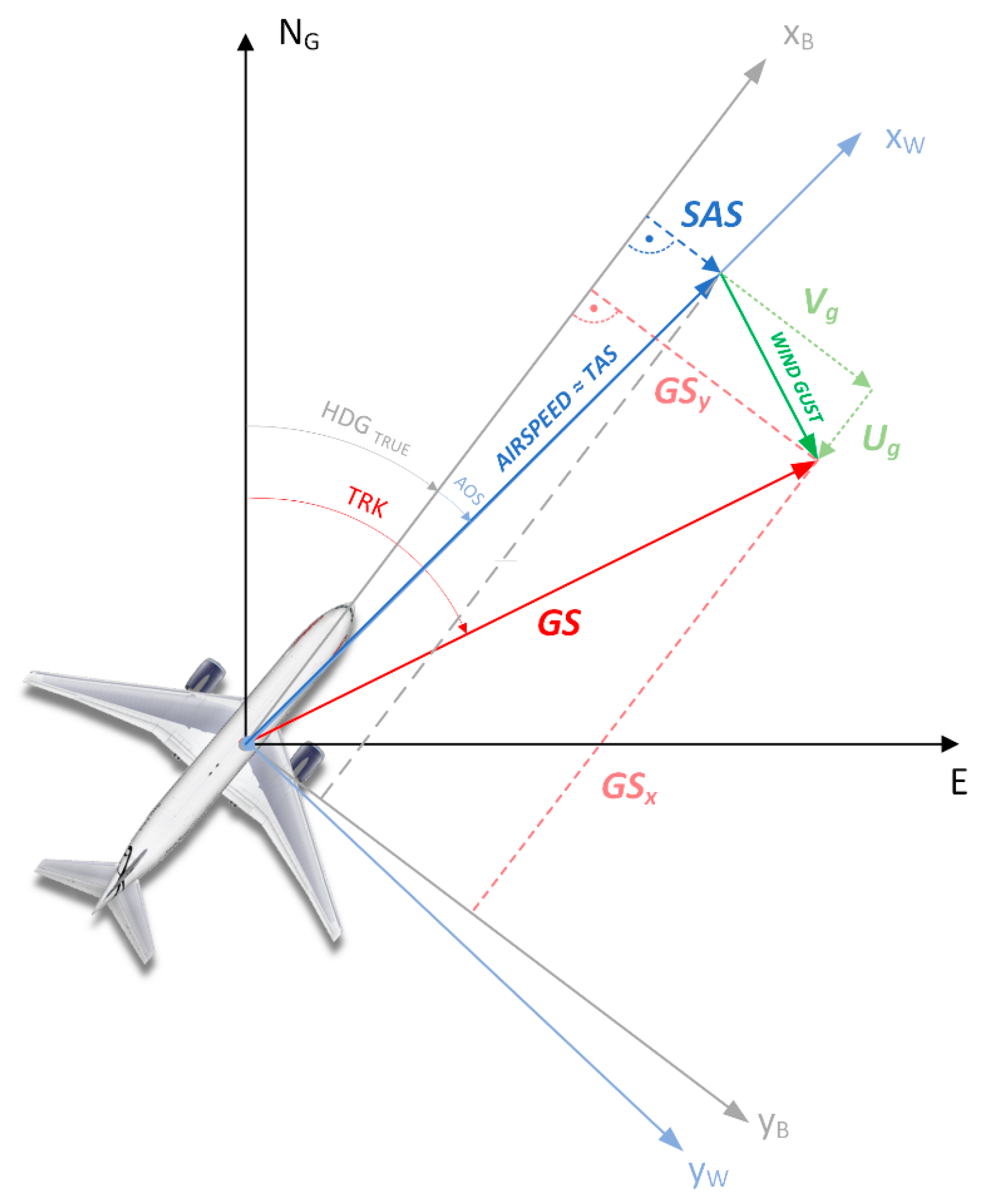
2.1. Analysis of the Possibilities of Wind Gusts Estimation (3D Problem)

The airplane’s mathematical model may take the form of equations describing its longitudinal and lateral motion [29,30]. Typically, these are two sets of linearized ordinary differential Equations (1) and (2).
d d t X l o n = A l o n · X l o n + B l o n · U l o n + C l o n · Z l o n
d d t X l a t = A l a t · X l a t + B l a t · U l a t + C l a t · Z l a t
The state variables are specified as follows for longitudinal and lateral motion, respectively:
X lon   =   ( u ,   w ,   q ,   ϑ ) T               X lat   =   ( v ,   p ,   r ,   φ ) T
The control (U) and disturbance vectors (Z) are defined as:
U lon   =   ( δ H ,   δ T ) T           Z lon   =   ( w g ,   u g ) T         U lat   =   ( δ a ,   δ f ) T           Z lat   =   ( V g ) T
The mathematical model of the aircraft presented here is built upon the principles of flight mechanics. The coefficient matrices (5)–(7) in the longitudinal motion, described by Equation (1), and lateral motion, described by Equation (2), include the respective aerodynamic derivatives.
A l o n = X u X w 0 g · cos θ 0 Z u Z w U 0 g · sin θ 0 M u M w M q 0 0 0 1 0   A l a t = Y v Y p Y r U 0 g · cos θ 0 L v L p L r 0 N v N p N r 0 0 1 tan θ 0 0
B l o n = X δ H X δ T Z δ H Z δ T M δ H M δ T 0 0             B l a t = Y δ A X δ R L δ A L δ R N δ A N δ R 0 0
C l o n = X w X u Z w Z u M w M u 0 0                 C l a t = Y v L v N v 0
The variation in gust values along the airplane’s longitudinal axis (ug) and vertical axis (wg) is reflected in the longitudinal motion, as shown in Equation (1), while changes in gust values along the lateral axis (vg) appear in the lateral motion in Equation (2). The gust parameters (ug, wg, vg) are included in the disturbance vectors Zlon and Zlat (4), respectively.
By substituting the matrices Alon, Blon, and Clon and the vectors Xlon, Ulon, and Zlon into Equation (1), we obtain four equations. The first, second, and third of these can be directly expressed as dependences (8)–(10). State variable ϑ, represented by the fourth of the equations, is the integral of the pitch angular velocity q. As a result, the described process is shifted in phase by 90 degrees, and consequently, there is an additional delay. For this reason, this equation will not be very useful for gust estimation tasks.
u ˙ = X u · u u g + X w · w w g g · ϑ · cos θ + X δ H · δ H + X δ T · δ T
w ˙ = Z u · u u g + Z w · w w g + U 0 · q g · ϑ · sin θ + Z δ H · δ H + Z δ T · δ T
q ˙ = M u ¯ · u u g + M w ¯ · w w g + M q ¯ · q + M δ H ¯ · δ H + M δ T ¯ · δ T
It is important to note that q, u, ug, w, wg, ϑ , δH, and δT represent changes in values, not absolute values. This is due to the fact that Equations (1) and (2) describe an incremental model. This characteristic was considered during the modelling of the estimation system. By assuming constant thrust (δT = 0), we reduce dependencies (8)–(10) to the forms (11)–(13):
u ˙ = X u · u u g + X w · w w g g · ϑ · cos θ + X δ H · δ H
w ˙ = Z u · u u g + Z w · w w g + U 0 · q g · ϑ · sin θ + Z δ H · δ H
q ˙ = M u ¯ · u u g M w ¯ · w w g + M q ¯ · q + M δ H · δ H
By transforming the dependencies (11) and (12) with respect to ug and wg, we obtain Equations (14) and (15):
u g = u 1 X u · u ˙ g X u · ϑ · cos θ + X δ H X u · δ H + X w X u · w w g
w g = w 1 Z w · w ˙ g Z w · ϑ · sin θ + Z δ H Z w · δ H + Z u Z w · u u g
The first two expressions on the right-hand side of Equations (14) and (15) indicate that the gust can be determined by knowing the changes in velocities u and w, as well as their first derivatives. Considering the effect of the change in the aircraft’s pitch angle and the deflection of the elevator is necessary to account for transient processes (larger time constants characterize the effect of gusts on the aircraft’s pitch angle change and the interaction of the pilot or autopilot in the longitudinal channel). The last terms in the sum of Equations (14) and (15) are related to the mutual (cross) interaction of head-on and vertical gusts in the longitudinal motion model of the aircraft.
Equation (13) holds great potential for developing an algorithm for estimating head-on and vertical gusts, as it relates their values to the pitch angular velocity q. This parameter is characterized by relatively small time constants in response to the occurring gusts. Equation (13) also includes the first derivative of q with respect to time, which is additionally characterized by a phase shift of −90 degrees. The only slow-varying parameter in this equation is the relationship linking the gust estimate with the aircraft’s response to the elevator deflection. After transformation with respect to ug and wg, Equation (13) takes the form of Equations (16) and (17). The results obtained in this work [28] suggest that Equation (16) can be used for estimating the fast-varying component of the head-on gust.
u g = u 1 M u ¯ · q ˙ + M q ¯ M u ¯ · q + M δ H M u ¯ · δ H + M w ¯ M u ¯ · w w g
w g = w 1 M w ¯ · q ˙ + M q ¯ M w ¯ · q + M δ H M w ¯ · δ H + M u ¯ M w ¯ · u u g
In this approach to the problem, the vertical and headwind gust estimation algorithms are mutually dependent. When attempting to determine gust values along only one of these axes, it can be simplified by assuming a one-dimensional gust. For example, in work [28], a dominant headwind gust was assumed. In this case, we can assume wg = 0 (no vertical gust) and W = const (the model is incremental; so, we can also assume w = 0). By introducing gain factors, Equation (16) transforms into Equation (18).
u g = u + k 1 u · q ˙ + k 2 u · q + k 3 u · δ H
Similarly, assuming the absence of headwind gusts, the value of the fast-varying components of the vertical gust can be estimated using Equation (19).
w g = w + k 1 w · q ˙ + k 2 w · q + k 3 w · δ H
Estimations of ug and wg will correspond to the high-frequency estimation of headwind (ug-hi) and vertical gust (wg-hi). This has been extensively discussed in the authors’ previous work [28].
Using the state Equation (2) for lateral motion, relationships (20)–(22) can be derived, linking the lateral gust vg to the linear velocity v and the angular velocities p and r in the aircraft’s body-fixed coordinate system. In these linearized state equations, the rudder deflection δR and aileron deflection δA are also variables.
v ˙ = Y v · v v g + Y p · p + Y r · r + Y δ A · δ A + Y δ R · δ R + g · cos θ 0
p ˙ = L v · v v g + L p · p + L r · r + L δ A · δ A + L δ R · δ R
r ˙ = N v · v v g + N p · p + N r · r + N δ A · δ A + N δ R · δ R
Equation (21) describes the aperiodic rolling motion, where the influence of the lateral gust is significantly smaller compared to its effect on the yaw rate r and the linear velocity v. For this reason, the analysis of Equation (21) was omitted, focusing instead on relationships (20) and (22). By transforming Equations (20) and (22) with respect to the lateral gust vg, we obtain Equations (23) and (24), respectively.
v g = v v ˙ Y v + Y p Y v · p + Y r Y v · r + Y δ A Y v · δ A + Y δ R Y v · δ R + g Y v · cos θ 0
v g = v r ˙ N v + N p N v · p + N r N v · r + N δ A N v · δ A + N δ R N v · δ R
By introducing gain coefficients in place of constant expressions in Equations (23) and (24), we obtain Equations (25) and (26). Preliminary research has shown that relationship (25) is particularly useful for estimating the fast-varying component of lateral gusts (vg-hi).
v g = v + k 1 v · v ˙ + k 2 v · p + k 3 v · r + k 4 v · δ A + k 5 v · δ R + k 6 v
v g = v + k 1 v · r ˙ + k 2 v · p + k 3 v · r + k 4 v · δ A + k 5 v · δ R
An advantage of estimating wind gust velocities using state equations is the ability to directly utilize measurement results obtained in the aircraft’s body-fixed coordinate system (FB). However, a drawback of this approach is the difficulty in estimating gust values in a three-dimensional framework (due to interdependencies in the algorithms) and its limitation to selected, identified flight states of the specific aircraft. These algorithms are also highly sensitive to the dynamic characteristics and errors of individual sensors [31,32], and the high-frequency signals ug-hi, vg-hi, and wg-hi, provided as high-pass input to the complementary filter, require corrections that are challenging to determine analytically [28]. For these reasons, estimating wind gusts in a 3D framework is very difficult and problematic to achieve using only state equations.
This paper proposes a complementary approach to the problem of gust estimation. It is assumed that analyzing measurements performed in three reference frames and correlating them can yield significantly better results, particularly for slow-varying signals. The chosen reference frames are the Earth-fixed frame (Fv), the airflow-fixed frame (Fw), and the aircraft-fixed frame (FB). Integrated measurement and navigation systems installed on commercial aircraft enable direct data acquisition in these reference frames (of course not globally, but specific variables only in selected reference systems). For example, the ADIRS system allows the determination of the aircraft’s velocity relative to both the Earth and the air mass. Additionally, using data from ADIRS accelerometers enables the measurement of accelerations and, subsequently, the calculation of velocity values (or changes) in the aircraft-fixed frame.
The complementary approach to the problem of three-dimensional gust estimation proposed in this paper does not require detailed modelling of the dynamic properties of the aircraft or as many simplifying assumptions as when using only state equations. However, state equations allow for a relatively accurate determination of the fast-varying gust components. The airflow movement along each axis was analyzed individually, enabling the development of methods for estimating both the slow-varying component (steady wind) and the fast-varying component (gusts). The specific methods are detailed in Section 2.2, Section 2.3 and Section 2.4.

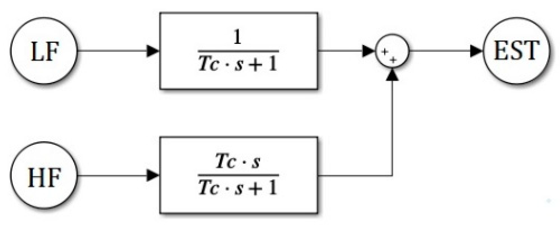
2.2. Proposed Methods for Estimating Head-On Gusts

The wind gust velocity component along the airplane’s longitudinal axis (Ug) can be determined by calculating the vector difference between the measured TAS and the ground speed component GSx along the airplane’s x-axis (27). A positive value of Ug indicates a headwind, where the wind is blowing directly toward the nose of the aircraft (Figure 2).
U g = G S x T A S
Using the dependencies presented in Figure 2 and knowing the true heading (HGDtrue) and track (TRK) angles, it is also possible to estimate not only the Ug component but also the direction and total speed of the wind, as well as lateral component of wind gust. This estimation is effective for gradual changes in wind speed and direction. Equation (27) can be easily derived from the general form presented in references [33,34,35,36]. TAS is measured on board the transport aircraft using systems such as the ADC (Air Data Computer) or ADIRU/ADIRS (Air Data Inertial Reference System). To determine the component GSx, it is necessary to measure the GS and true track (TRK), as well as the aircraft’s true heading (HDGtrue). These data can be obtained through the satellite navigation system (GNSS) and/or the ADIRU/ADIRS system. TAS and GSx measurements exhibit significant inertia and time constants, which can last several seconds, depending on the system structure, sensors, and algorithms. Consequently, the estimation of Ug can be associated with the low-frequency component of headwind estimation (Ug-lo), as indicated by identity (28).
U g l o U g
Dangerous wind gusts are typically marked by rapid changes, and to estimate them, it is essential to consider the fast-changing state variables. The research hypothesis of this study posits that the proposed method for estimating the headwind component, as described by Equation (27), along with the transient changes in its value (gusts) outlined in Equation (18), can be effectively used in a complementary manner. Equation (27) serves to determine the overall value of the wind speed in the form of the headwind component.
The measurement characteristics of GS and TAS, particularly their significant delays, impose strict limitations on the rapid and precise detection of gusts. While Equation (18) can estimate short-term variations in the headwind component, it cannot provide its absolute value. A practical solution to address this challenge is the implementation of a complementary filtering system. The complementary filter (CF) is a cost-effective and efficient data fusion technique that integrates a low-pass filter with a high-pass filter [37]. The general structure of the CF (Figure 3) incorporates low- and high-frequency inputs from the composite signal.
The transfer function of the complementary filter is expressed by Equation (29). Across the entire frequency spectrum, the linear CF maintains a unity amplitude (0 dB magnitude). Additionally, the phase shift remains linear and is equal to 0 degrees (Figure 4).
E S T = 1 T c · s + 1 · L F + T c · s T c · s + 1 · H F
  • LF—low-frequency signal,
  • HF—high-frequency signal,
  • EST—output of CF.
On the basis of dependencies (18) and (27), the complete law of headwind estimation (including temporary gusts), can be formulated as (30) and, finally, as Equation (31).
U g e s t _ C F = 1 T c u · s + 1 · U g l o + T c u · s T c u · s + 1 · u g h i
U g e s t C F = 1 T c u · s + 1 · G S x T A S + + T c u · s T c u · s + 1 · ( u + k 1 u · q ˙ + k 2 u · q + k 3 u · δ H )
After assuming u = 1 s · a x and neglecting the model parameters that depend on the flight state, this can be expressed by approximation (32). Omitting several quantities related to the aircraft’s response to a gust may seem radical and unjustified; however, as established in [28] based on a quantitative analysis of the obtained results, a complementary filter time constant of approximately 1 s yields the best results for this estimation. The fastest response to a gust is achieved through the direct measurement of longitudinal acceleration ax (a primary-type response). The other omitted quantities, such as q ˙ , q , and δ H , exhibit a secondary nature.
U g e s t _ C F   1 T c u · s + 1 · G S x T A S + T c u · a x T c u · s + 1
The methodology for selecting complementary filter parameters and evaluating the obtained results was described in detail in our previous work [28], which concerned the estimation of gusts in the longitudinal axis only.

2.3. Proposed Methods for Estimating Side Gusts

Assuming a coordinated flight without sideslip, the crosswind component along the aircraft’s lateral axis can be estimated based on the ground speed component measured along the yB-axis of the aircraft’s body-fixed coordinate system (GSy, Figure 2). A positive Vg value indicates wind blowing from the left side of the aircraft (opposite to the direction of the yB-axis).
V g l o   = G S y   = G S · sin ( T R K H D G T R U E )
In the case of analyzing the lateral gust component, the sideslip angle can play a significant role. Figure 5 illustrates the relationships between the TAS vector measured in the aircraft-fixed coordinate system (FB), the AIRSPEED vector representing the actual velocity of the aircraft in the air-mass-fixed coordinate system (reference frame Fw) [38] and the GS velocity relative to the ground (reference frame Fv). By considering the angle of sideslip (AOS), the sideslip airspeed (SAS) can be determined:
S A S = T A S · sin ( A O S )
By incorporating relationships (33) and (34), the value of the gust Vg can be calculated using the following equation:
V g l o   = G S y S A S = G S · sin T R K H D G T R U E T A S · sin ( A O S )
Determining the GSy component requires measuring GS, track angle (TRK), and the aircraft’s heading (PSI), as in the case of longitudinal gust estimation. To calculate the lateral velocity in a sideslip, it is necessary to measure the angle of sideslip (AOS) and true airspeed (TAS). Similar to the previously discussed estimation methods, to enhance the accuracy of estimations during sudden and turbulent gusts, the use of a high-frequency signal was also adopted. For this purpose, the lateral acceleration component provided by accelerometers integrated into the ADIRU systems, which are part of the aircraft’s onboard systems, was utilized. While this signal is not suitable for estimating the total value of the crosswind, integrating the lateral acceleration enables relatively precise determination of the component for sudden and short-lived lateral gusts.
In the continuation of work on developing a three-dimensional gust estimation algorithm, including lateral gusts, it was decided to retain the use of complementary filtering, which yielded the most favorable results during the studies on headwind gust estimation [28]. Based on dependencies (25) and (35), the complete law of sidewind estimation (including temporary gusts) can be formulated as Equations (36) and (37).
V g e s t _ C F = 1 T c v · s + 1 · V g l o + T c v · s T c v · s + 1 · v g h i
V g e s t C F = 1 T c v · s + 1 · G S · sin T R K H D G T R U E T A S · sin ( A O S ) + + T c v · s T c v · s + 1 · ( v + k 1 v · v ˙ + k 2 v · p + k 3 v · r + k 4 v · δ A + k 5 v · δ R + k 6 v )
After assuming v = 1 s · a y , neglecting constant values on the input of hi-pass filter, as well as the model parameters that depend on the flight state, this can be expressed by approximation (38).
V g e s t C F 1 T c v · s + 1 · G S · sin T R K H D G T R U E T A S · sin A O S + + T c v · a y T c v · s + 1

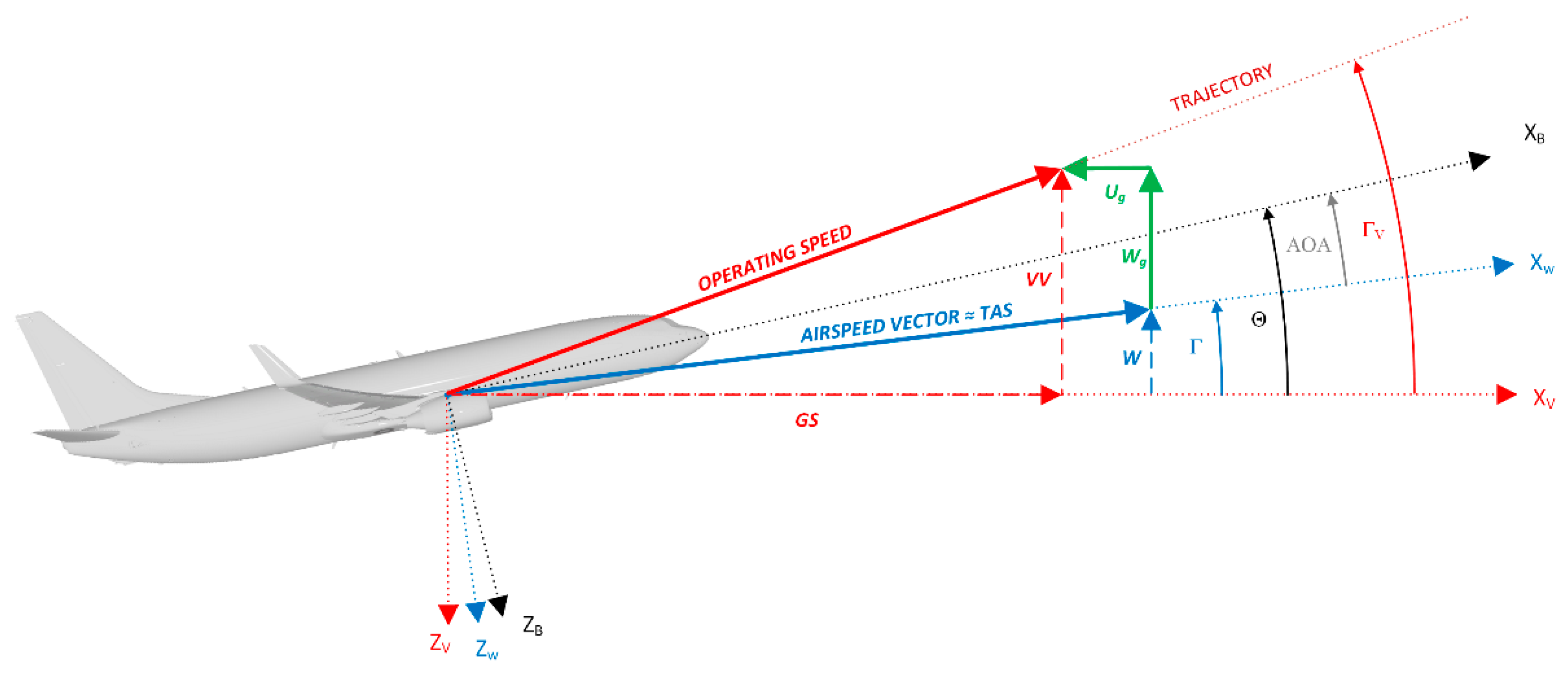
2.4. Proposed Methods for Estimating Vertical Gusts

The vertical wind gust component along the aircraft’s vertical axis can be estimated based on the difference between the aircraft’s vertical velocity W, resulting from its flight path angle relative to the vertical motion of the air mass, and the vertical velocity VV (ground relative velocity measured by the variometer along the zV-axis; Figure 6). A positive Wg value indicates upward wind (opposite to the direction of the zV). Equation (39) defines the slowly varying (quasi-steady state) component of the vertical gust, assuming the simultaneous occurrence of a headwind gust.
W g l o   = VV W = VV TAS · sin Γ = V V T A S · s i n Θ A O A
In commercial aircraft, the measurement of the flight path angle is performed using indirect methods. For the purpose of vertical gust estimation, an ideal measurement of the flight path angle from a simulation environment was used as input data in this study. In practice, the flight path angle can be determined in various ways, as presented in numerous studies [39,40].
On the basis of dependencies (19) and (39), the complete law of vertical wind estimation (including temporary gusts), can be formulated as (40) and (41).
W g e s t _ C F = 1 T c w · s + 1 · W g l o + T c w · s T c w · s + 1 · w g h i
W g e s t C F = 1 T c w · s + 1 · V V T A S · sin Θ A O A + + T c w · s T c w · s + 1 · ( w + k 1 w · q ˙ + k 2 w · q + k 3 w · δ H )
After assuming w = 1 s · a z and neglecting the model parameters that depend on the flight state, this can be expressed by approximation (42).
W g e s t C F 1 T c w · s + 1 · V V T A S · s i n Θ A O A + T c w · a z T c w · s + 1

3. Research Environment and Plan of Experiment

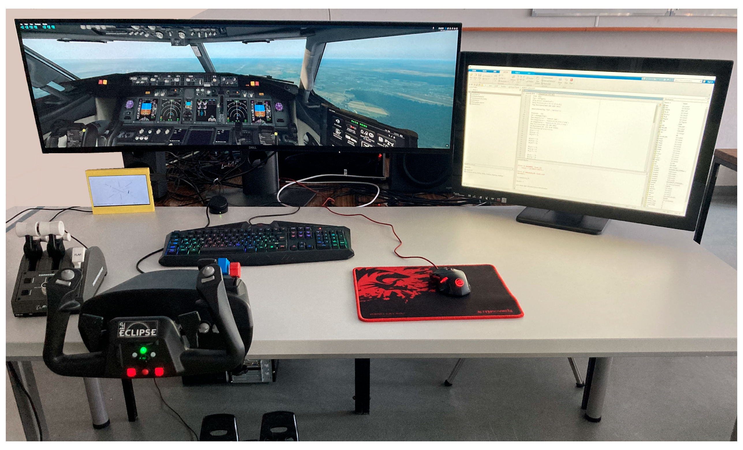
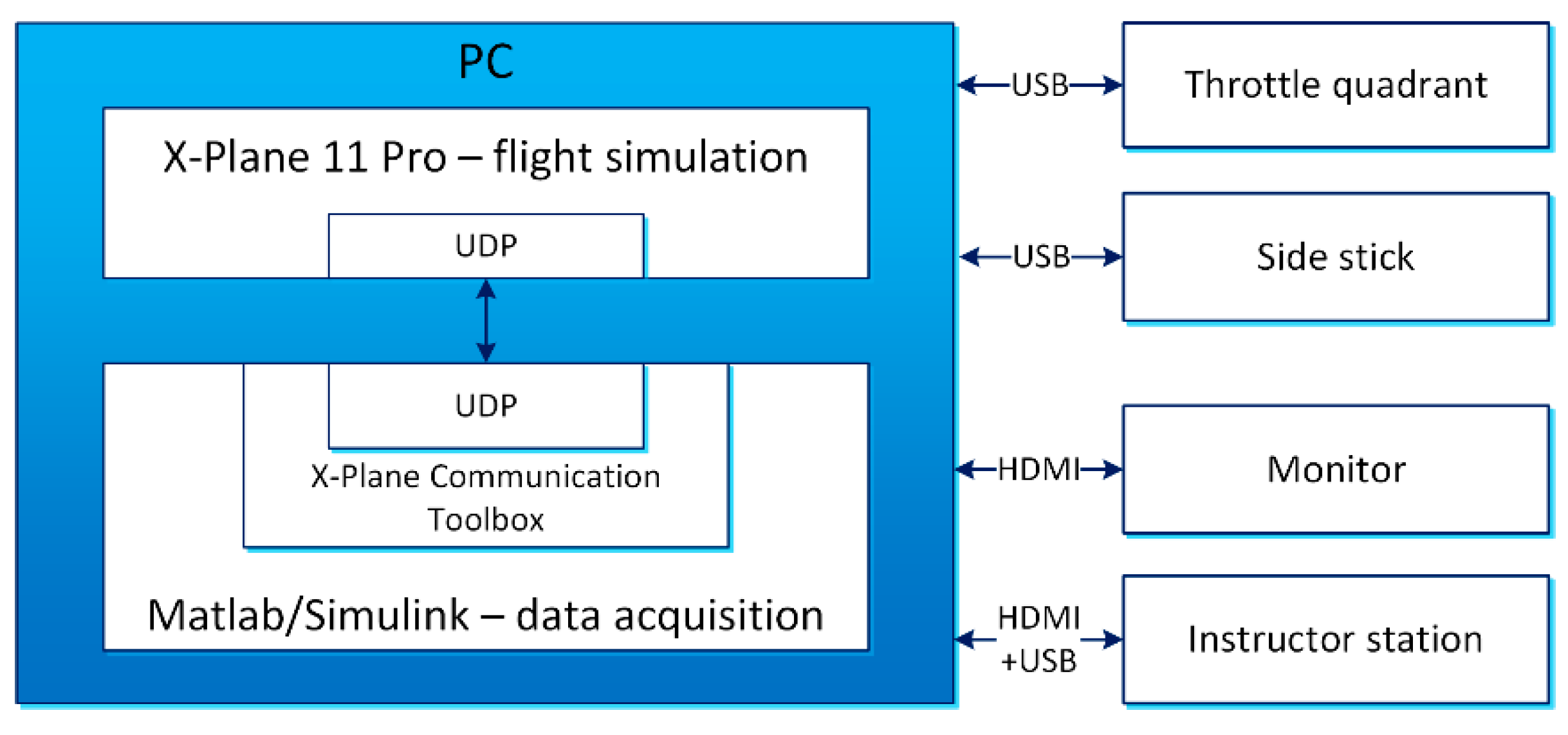
3.1. Flight Simulation Environment and Data Acquisition

A simulator station (Figure 7) was used to evaluate the potential of estimating gust values using the algorithms described in Section 2. The external components of the simulator and their connection are presented on the block diagram (Figure 8). A professional and certified version of the X-Plane 11 Pro software was utilized, enabling enhanced use of the environment’s features for research purposes. The weather configuration tool within X-Plane allowed for the generation of wind layers from selected directions. It was possible to define both a constant wind speed and the intensity of gusts generated by the simulator environment. Experimental simulator flights were conducted using a realistic model of the widely used medium-range narrow-body aircraft the B737-800 (Figure 9). This advanced model accurately reflects the aircraft’s dynamic characteristics and operational behavior. A major advantage of the selected software is its ability to record all flight parameters required by the estimation methods under consideration. Table 1 presents a comprehensive overview of the recorded flight parameters, encompassing all potentially accessible physical data sources.
The developed estimation algorithms required the recording of both weather parameters and data from various on-board aircraft’s systems, including the: ADIRU, GPS, FCC (Flight Control Computer). More advanced data were not accessible via X-Plane’s built-in user interface and instead required referencing X-Plane internal data structures (Datarefs). To accomplish this, the X-Plane Communication Toolbox (XPC) [41] was used to record all flight parameters. XPC was initialized and configured in the Matlab/Simulink environment. This setup enabled the recording and retrieval of internal variables using the UDP protocol (Figure 8).
The X-Plane 11 Pro software employs a sophisticated nonlinear model to simulate aircraft dynamics [42]. This model utilizes blade element theory, which divide the aircraft into numerous small elements and calculates the aerodynamic forces acting on each element at frequencies ranging from several to dozens of hertz [43,44]. It accounts for complex environmental factors, including various wind phenomena, such as gusts. Wind parameters (direction, speed, and gust intensity) can be configured independently for each atmospheric layer via the instructor’s station module (shown on the right in Figure 8). During data recording, the wind output parameters are stored in the OpenGL coordinate system, which is Earth referenced (illustrated by the red arrows in Figure 10). For the purposes of this study, these parameters were converted into the aircraft’s body-fixed coordinate system. As a result, the Ug, Wg, and Vg wind components were determined (represented by blue arrows in Figure 10).
In the conducted research, the X-Plane 11 Pro simulator provided three categories of data to the Matlab/Simulink environment:
Indications from flight instruments (cockpit indicators),
  • Data from simulated avionics systems (flight model controls and flight model position),
  • Real-time gust parameters generated by predefined wind layers (simulation weather).

3.2. Simulation Assumptions

The simulations were conducted under the following assumptions:
  • Aircraft weight: 65,000 kg,
  • Automatic flight with a layer of atmospheric gusts
  • Three flight phases: descent, level flight and climb
  • Simulation performed by a pilot holding a current type rating for the B737.
Automatic simulated flights were carried out using the following autopilot and autothrottle modes:
  • LVL CHG (Level Change). This mode coordinates pitch and thrust commands to perform automatic climbs and descents to preselected altitudes at specified airspeeds. During descent, the autothrottle mode annunciates RETARD, followed by ARM, and then maintains the idle thrust. During the climb, the autothrottle mode annunciates N1 for climb and holds limit thrust for CLB from FMC. In both cases, the Autopilot Flight Director System (AFDS) holds the selected airspeed [45]. The rate of climb is a resulting parameter. This mode allows for the assumption of approximately constant thrust during simulation (the VS—Vertical Speed mode maintains a constant vertical speed, adjusting thrust and pitch to hold the selected IAS and vertical speed VVI).
  • ALT HLD (Altitude Hold). In this mode, the autopilot commands pitch to hold the uncorrected barometric altitude at which the switch was pressed or MCP (Mode Control Panel) selected altitude after climb or descent. The autothrottle system holds the selected speed indicated in the IAS/MACH display on the MCP by adjusting the throttle control and thrust accordingly.
  • HDG SEL (Heading Select). This mode commands roll to turn to and maintain the heading set on the MCP HEADING display. The maximum bank angle limit is limited by the bank angle selector [45].
The amplitudes of simulated gusts used in the tests were determined (taking into account the limitations of the simulation environment) based on empirical data and documented reports [46,47]. Peak values of headwind changes or downdrafts may slightly exceed the design gust envelopes defined in CS-25 and FAR 25 [48,49], but they remain valid for simulating extreme transient events. The gust amplitudes used in the simulations are considered physically plausible and appropriate for modeling extreme yet credible scenarios—particularly those associated with terrain-induced gusts, thunderstorms, or microburst conditions.

3.3. Flight Plan and Its Realisation for Estimating Head-on Gusts

During the simulation, the aircraft descended from an altitude (ALT) of 14,000 ft (4267.2 m) to 6000 ft (1828.2 m). The flight was fully automated with the pilot operating the autopilot and autothrottle systems in LVL CHG and HDG SEL modes. A constant IAS 250 kt (128.6 m/s) was set on the MCP. Basic flight parameters are presented in Figure 11. Significant IAS fluctuations occurred between 50 s and 340 s of the recording (Figure 12B), caused by variable atmospheric gusts. These gusts also had a substantial impact on the aircraft’s vertical speed (VVI), which varied from a stabilized 6 m/s at the start of descent to values ranging between 3 and 12 m/s.
The wind conditions were calm above 14,000 ft (4267.2 m) and below 6000 ft (1828.2 m). As the airplane descended below 4000 m, the headwind speed Ug began to increase, as shown in Figure 12A,B. When wind speeds exceeding 3 m/s, sudden gusts with peak velocities up to 22 m/s were observed. These occurred between the 50th and 320th seconds of the simulation. From 320 to 350 s, both headwind and gust intensity gradually decreased, eventually returning to calm conditions below 1828.2 m.
A subsequently simulated level flight was conducted within a wind layer containing head-on gusts at a constant altitude of 10,000 ft (Figure 13 and Figure 14). Due to limited simulator environment capabilities there were no possibilities to set the wind layer at a specific location in the horizontal plane. As a result, the recording does not include calm wind conditions at the beginning or the end of the flight segment. The level flight was executed automatically using the autopilot ALT HLD mode with MCP selected speed of 250 kt (128.6 m/s). Due to the presence of strong head-on gusts ranging from 5 to 22 m/s, significant variations in IAS were observed. Despite this, the altitude stabilized within 20 m, while the vertical speed fluctuated between −2 and 2 m/s.
The next simulation was conducted for an aircraft climbing through a layer of head-on gusts, from 6000 ft (609.6 m) to 14,000 ft (4267.2 m) (Figure 15 and Figure 16). Wind conditions were calm below 6000 ft (1828.2 m) and above 14,000 ft (4267.2 m). During the climb the speed of head-on wind increased with maximum gusts up to 19 m/s. After passing 3750 m, the wind speed decreased until reaching windless conditions and the end of climb.
The climb was performed using the autopilot LVL CHG mode with a constant IAS 250 kt (128.6 m/s) set on MCP. At the start of the climb, the vertical speed stabilized at about 25 m/s, then it started to fluctuate due to atmospheric gusts. The total simulation time was approximately 50% shorter compared to the descent scenario, owing to the significantly higher vertical speed enabled by the high thrust setting.

3.4. Flight Plan and Its Realisation for Estimating Side Gusts

To continue the development of the lateral gust estimation algorithm, a similar simulation methodology was employed. The aircraft was flown through a programmatically generated layer of gusts with a constant direction set at 90 degrees to the flight path. This configuration allowed for the simulation of ideal side gusts (with minimal frontal components and no vertical components). The minimally increasing frontal components resulted from the autopilot maintaining a given constant heading in the HDG SEL mode. As the drift angle was formed due to the increasing crosswind and increasingly stronger atmospheric gusts, small head-on gust components appeared.
During the simulation, the aircraft descended from an altitude (ALT) of 12,000 ft (3660 m) to 6000 ft (1829 m) (6000 ft). The flight was fully automated using the autopilot in LVL CHG mode. Basic flight parameters are shown in Figure 17. IAS fluctuations at the beginning and at the end of simulation in relation to the set speed of 250 kt (128.6 m/s) were caused by changes in flight phases: during the first 30 s of simulation—the transition from level flight to descent and from 280 s to 300 s—the transition from descent to level flight. The vertical speed during descent was the result of the MCP setting and logic of LVL CHG mode and was approximately 1380 ft/min (7 m/s). Minor fluctuations in the vertical speed were also caused by variable atmospheric side gusts and by changes in flight phases.
At an altitude of 3660 m (12,000 ft), wind conditions were calm. After the descent commenced from this altitude, the crosswind (Vg) began to increase. Between the 75th and 240th seconds of the recording, once the crosswind exceeded the speed of 4 m/s, sudden lateral gusts occurred reaching peak velocities of up to 23.5 m/s (Figure 18A,B). After passing 2600 m, side gusts started to decrease. From 2200 m to 1828.2 m (6000 ft), the crosswind gradually diminished until wind conditions became calm again.
Subsequently, the test pilot performed simulated level flight through a crosswind layer containing lateral gusts. The autopilot and autothrottle systems were engaged in ALT HLD and HDG SEL modes with a constant altitude of 10,000 ft (3048 m) selected on the MCP. During simulation, only small fluctuations in the altitude, IAS, and vertical speed were recorded (Figure 19). On this basis, it can be concluded that side gusts had no significant impact on these three basic flight parameters.
As shown in Figure 20, side gusts generated by the simulator environment were highly dynamic, with gusts velocities increasing sharply from 6 m/s to 21 m/s over a short time interval. Similar to the level flight simulations involving head-on gusts, this flight was performed in crosswind layer without initial or final calm wind conditions. Minor frontal headwind components (below 2 m/s) occurred because of maintaining a constant heading in autopilot HDG SEL lateral mode. No vertical gusts components Wg were observed during the simulation.
The next simulation was conducted to evaluate the proposed method for estimating side gusts during the climb phase (Figure 21 and Figure 22). The Boeing 737–800 was climbing from 6000 ft (1828.2 m) to 14,000 ft (4267.2 m). At these specified altitudes, the wind was calm. Above an altitude of 2250 m, the crosswind exceeded 3 m/s, and side gusts with a maximum speed up to 21 m/s started to appear (Figure 22A,B). After passing 4000 m, the gusts ceased, and the crosswind speed gradually decreased until windless conditions were reached at the end of the climb. No vertical gusts Wg were observed throughout the climb. Minor frontal headwind components (below 2 m/s) occurred because of maintaining a constant heading in autopilot HDG SEL lateral mode. Figure 20 presents the selected flight parameters during the climb phase. The initial increase in IAS speed after 20 s of recording was caused by the autothrottle system transitioning from MCP SPD mode to N1 mode during the start of climb in LVL CHG mode. Analyses in Figure 21 reveal that side gusts had only a minor influence on IAS and vertical speed. The vertical speed during the climb was approximately constant (about 20 m/s) compared to the significant changes that could be observed while passing through the head-on gust layer.

3.5. Flight Plan and Its Realization for Estimating Vertical Gusts

The simulator environment lacked the capability for the selection of vertical gust parameters. This highlights the constraints of flight simulator assumptions in this context and emphasizes the necessity for more in-depth research into this phenomenon. However, a vertical gust component was present in the microburst simulation model, which included both frontal and lateral wind components. Microbursts could be introduced during any flight phase selected via the instructor station module.
The simulations were conducted under the following additional assumptions:
  • Constant thrust was maintained during level flight prior to the occurrence of a microburst,
  • Variable thrust as the autothrottle control system responds to a microburst,
  • Simultaneous occurrence of side and frontal wind components in the available microburst model.
The first microburst simulation was conducted during descent, which was also performed using LVL CHG mode (Figure 23 and Figure 24). During the descent from an altitude of 12,000 ft (3658 m) to an altitude of 8000 ft (2439 m), 104 s after the start of the simulation, at an altitude of 10,000 ft (3048 m), a microburst was generated. Figure 24 shows the microburst parameters in the aircraft-related coordinate system and the vertical gust profile as a function of altitude. Analyzing both the flight parameters and the values of the microburst components, it can be noticed that the strongest frontal gusts of all the recordings (reaching 30 m/s) did not cause such a large decrease in the IAS speed as in the later microburst simulation during the descent (IAS speed decrease by 27 m/s for Ug max = 28.9 m/s vs. IAS speed decrease by 42 m/s for Ug max = 25 m/s). The crosswind components in the presented microburst model were minor, with a maximum speed of 2.4 m/s. The peak vertical gust reached 5.35 m/s. Under windless conditions, the vertical speed was 6.6 m/s, increasing to 10.8 m/s during the microburst.
This may indicate the reduced inertia of the aircraft during descent, making it easier for the automatic control systems to counteract the loss of speed. However, it is associated with a risk resulting from a visible increase in descent (120 s of simulation). In such circumstances, the risk of accident increases as the altitude above the terrain decreases. A sudden increase in vertical speed combined with a drop in IAS speed leads to a greater descent gradient and, consequently, a steeper angle of descent. This can trigger EGPWS warnings, necessitate a terrain escape maneuver, or even result in a catastrophic outcome.
During the next simulation (Figure 25 and Figure 26), the aircraft was flying at a constant altitude of 10,000 ft (3048 m). The flight was performed fully automatically using the autopilot mode—ALT HLD with a selected constant IAS speed of 250 kt (128.6 m/s).
During the first stage of the flight, at an altitude of 10,000 ft, there was no wind. Fifty seconds into the simulation, after the flight parameters were stabilized, a sudden microburst was triggered from the instructor station. Wind began increasing simultaneously in three axes (Figure 26). The headwind speed (Ug) increased, peaking at 22 m/s, then it started to decrease, shifting to a tailwind at the 55th second of the simulation. The tailwind at the extreme also reached a speed of 22 m/s, decreasing to zero 20 s after the microburst occurred. At the same time, a much weaker lateral gust was observed, with a peak value of only 1.8 m/s and changing direction throughout the event. A highly hazardous downdraft developed, with the vertical gust speed increasing to 9.6 m/s (1890 ft/min), then decreasing to zero by the 70th second of the simulation. The speed of vertical gust increased until it reached 9.6 m/s—(1890 ft/min) and then decreased to zero in the 70th second of the simulation. The microburst phenomenon poses a significant threat to flight safety due to the combination of a downdraft and the shift from a headwind to a tailwind. The occurrence of such sudden and varied atmospheric gusts caused significant changes in flight parameters (Figure 25). Returning to the pre-microburst condition required a significant amount of time. The automatic control systems restored the flight parameters to the values set before the microburst occurred, 30 s after the gusts had ceased.
The third microsquall simulation with flight parameter recording, was conducted during a climb in LVL CHG autopilot mode. After initiating a climb from an altitude of 8000 ft (2439 m) and stabilizing flight parameters, a microburst was generated from the instructor station at an altitude of 10,000 ft (3048 m), 68 s after the simulation began (Figure 27). In this case, the downdraft reached a maximum of 6.1 m/s (1200 ft/min), while the frontal and then rear gusts reached 25 m/s. The observed lateral gust was minor, with a maximum value of 2 m/s, and shifted direction during its occurrence (Figure 28). The microsquall occurred between 68 and 96 s of the simulation; during this time, the aircraft was climbing from 3048 m to 3400 m. Once the wind subsided, the aircraft completed its climb to an altitude of 3658 m (12,000 ft) and stabilized in level flight.
Given the steady increase in altitude and climb rate, it may seem that a microsquall does not pose a significant threat during this phase of flight. However, it is important to highlight the substantial decrease in IAS speed—drop of 42 m/s from 128.6 m/s to 86.6 m/s. By comparison, in level flight, the IAS decreased by nearly 20 m/s to 108.7 m/s, despite the slightly weaker frontal gust (Ug = 22 m/s versus 25 m/s during climb). This sharp drop in IAS during climb, especially when occurring shortly after takeoff at lower airspeeds, can be critical. A loss of this magnitude may lead to an aerodynamic stall, posing a serious risk to flight safety.

4. Results and Discussion

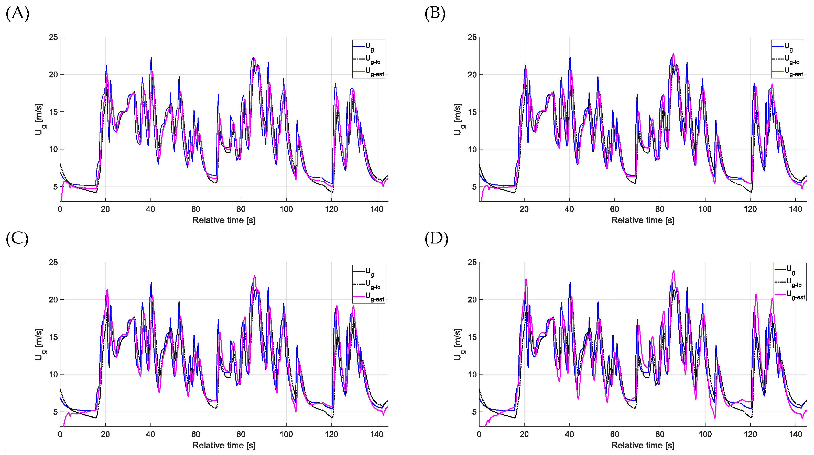
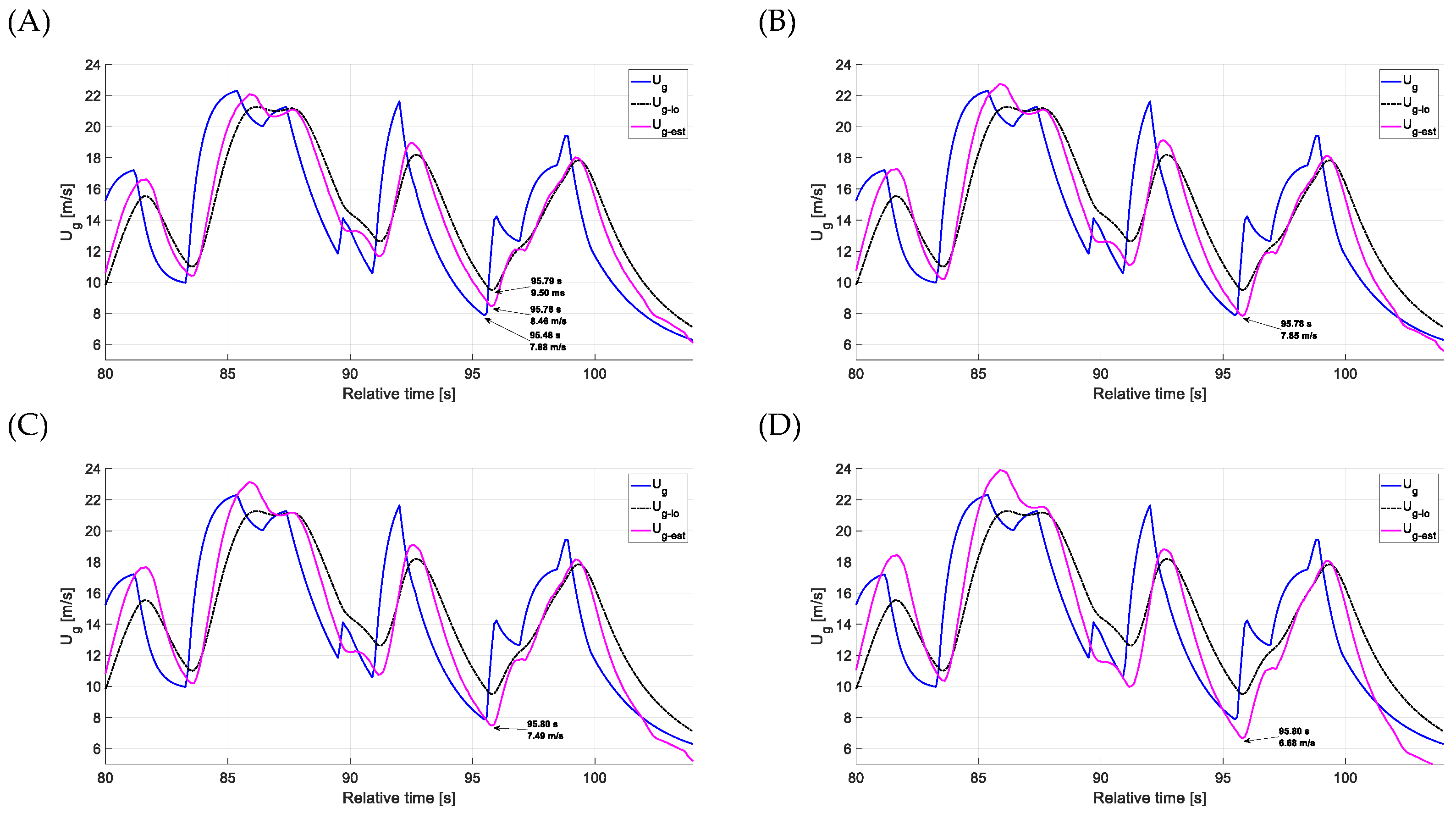
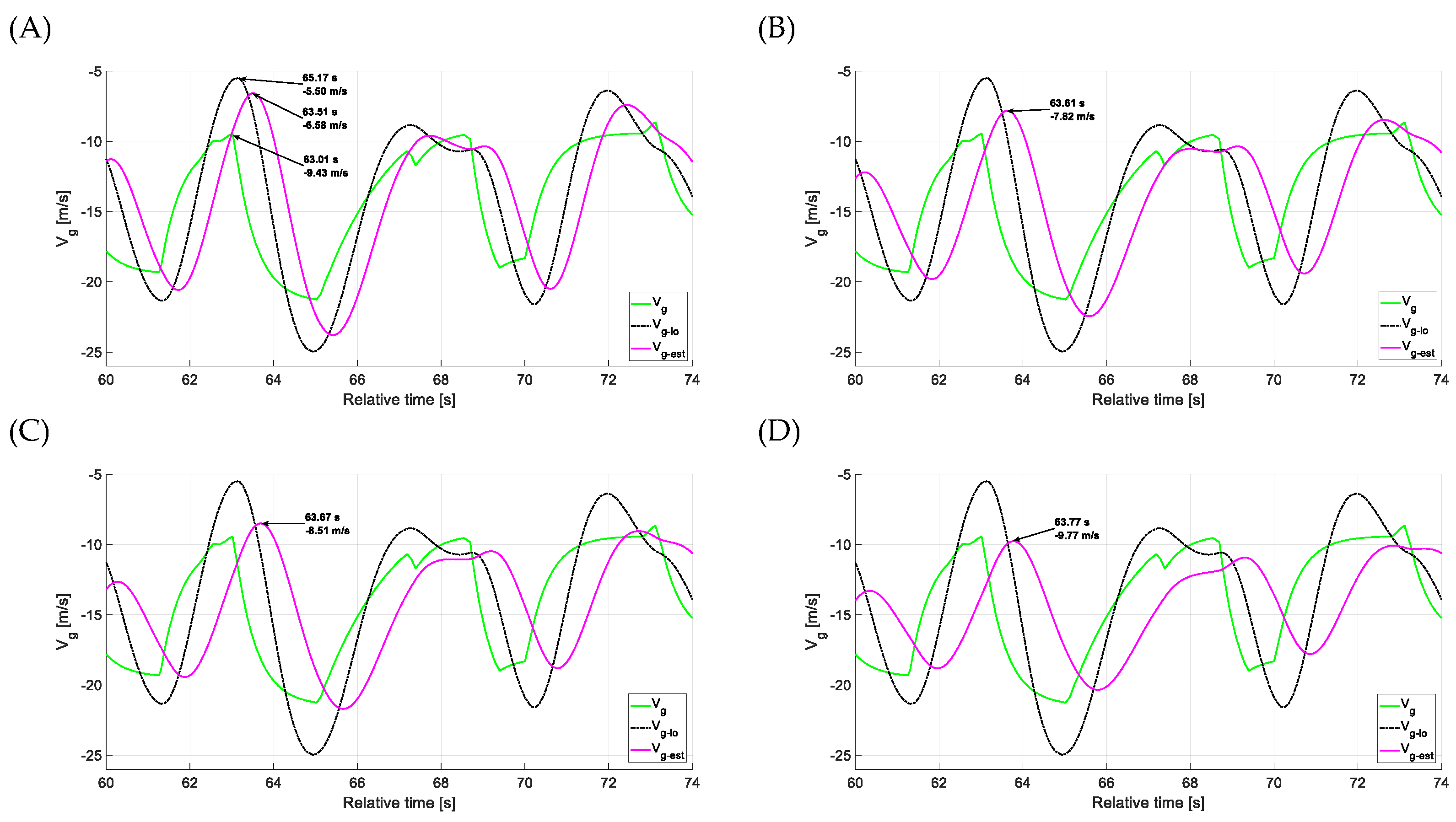
4.1. Estimation Accuracy—Head-on Gusts

The graphs in this section compare the ideal measurement scenario with the obtained low-frequency signal (Ug-lo) and the complete estimation (Ug-est). The latter combines low-frequency and high-frequency signals using a complementary filter (CF) across three analyzed flight phases.
The first flight phase examined was descent. Three data ranges were selected for graphical analysis: the entire simulation (0–330 s), a series of selected gusts (200–255 s), and a single gust event (220–238 s). The CF results illustrate the effect of varying the time constant Tcu on the estimation outcome. For comparison with the recorded gusts, four selected values of time constant—{0.5 s, 0.8 s, 1 s, 1.5 s}—were taken into account.
Based on Figure 29, Figure 30 and Figure 31, it can be concluded that the most accurate estimation results compared to the reference measurement, were obtained with time constants of 0.8 s and 1.0 s. Increasing the time constant from 0.5 s to 0.8 s improved the alignment between the estimation and the ideal headwind gust measurements. Taking a closer look on the arrows annotated with numerical data for the selected increasing gust in Figure 30, a computational comparison could be made. For the time constant of 0.5 s, the peak gust value is 0.64 m/s lower than the reference measurement for complete estimation (for low-frequency estimation this diffrence is more significant and amounts to 2.03 m/s). The delay of the full estimation in relation to the reference measurement is relatively small and is equal to 0.39 s, which is a better value in relation to the delay of the low-frequency estimation, which equaled 0.5 s. Increasing the time constant to 0.8 s allowed for an almost perfect match (0.02 m/s diffrence between the reference measurement) of the peak gust value considered while maintaining the full estimation delay of 0.39 s. Analysis of the numerical annotations of the arrows in Figure 31 allows for an accurate comparison of the minimum numerical values for the selected weakening gust case. Starting from a time constant of 0.5 s, the differences in the minimum value are 0.37 m/s for the full estimation and 0.84 m/s for the low-frequency estimation. The delays with respect to the reference measurement are 0.95 s for the full estimation and 1.39 s for the low-frequency estimation. When comparing the changes in the full estimated values for this selected case, the closest value to the reference measurement was achieved for a time constant of 0.8 s (only 0.04 m/s difference), while maintaining the delay at the level of 0.95 s. A time constant of 1.0 s already underestimates the minimum value by 0.2 m/s, while a time constant of 1.5 s underestimates it by 0.34 m/s, also increasing the estimation delay to 1.05 s.
For the considered cases of a gust with increasing velocity and a gust with decreasing velocity, the best results were obtained for a time constant of 0.8 s. However, the overall fit should also be taken into account for the final evaluation and conclusions. In this respect, the results for a time constant of 1.0 s are also satisfactory. On the other hand, an increase in the time constant to 1.5 s led to an overestimation of the peak gust values both in assessment and computational comparison of charts.
Subsequently, the estimation results for the simulation performed during level flight were analyzed. Three data ranges were selected for graphical representation: the entire simulation (0–143 s), a series of selected gusts (65–115 s), and a single gust (80–105 s). As in the previous case, the complementary filter (CF) results reflect the influence of varying the time constant Ts on the estimation performance. The same four time constants—{0.5 s, 0.8 s, 1 s, and 1.5 s}—were used for comparative analysis.
The evaluation of charts presented in Figure 32, Figure 33 and Figure 34 leads to the conclusion that the best representation of the estimation results compared to the reference measurement was obtained for the time constant of 0.8 s. By examining the arrows annotated with numerical values for the selected rising gust speed in Figure 33, a computational comparison can be made. When using a time constant of 0.5 s, the peak gust value is 0.2 m/s lower than the reference measurement in the full estimation, with a more pronounced difference of 1.04 m/s in the low-frequency estimation. The full estimation shows a relatively small delay of 0.5 s compared to the reference, which is an improvement over the 0.7-s delay observed in the low-frequency estimation. Increasing the time constant to 0.8 s leads to a peak value that exceeds the reference by 0.46 m/s, while still maintaining the 0.5-s delay in the full estimation. However, further increases in the time constant to 1.0 and 1.5 s resulted in progressively worse numerical performance. Reviewing the numerical labels on the arrows in Figure 34 enables a precise comparison of the minimum values for the selected decaying gust scenario. With a time constant of 0.5 s, the minimum value deviates by 0.58 m/s in the full estimation and by 1.62 m/s in the low-frequency estimation. The corresponding delays relative to the reference measurement are 0.3 s and 0.31 s, respectively. Among the full estimation results, the closest match to the reference is observed at a time constant of 0.8 s, differing by just 0.03 m/s and keeping the delay at 0.3 s. Increasing the time constant to 1.0 s results in an underestimation of 0.39 m/s, while a time constant of 1.5 s leads to a larger underestimation of 1.2 m/s and a slight delay increase to 0.32 s.
For both the increasing and decreasing gust scenarios, the most accurate results were achieved with a time constant of 0.8 s. Nonetheless, the overall match between the estimated and reference data should also be considered in drawing final conclusions. Conversely, raising the time constant to 1.5 s resulted in an overestimation of peak gust values, as seen in charts as well as in numerical analysis.
The third case analyzed for evaluating the headwind estimation algorithm using complementary filtering was climbing through a layer of head-on gusts. Three data ranges were chosen for graphical presentation: the entire simulation (0–190 s), a series of selected gusts (55–120 s), and a single gust (55–80 s).
Figure 35, Figure 36 and Figure 37 indicate that time constants of 0.8 s and 1.0 s provided the most accurate estimation results relative to the reference measurement. Analyzing the arrows labeled with numerical values for the selected rising gust speed in Figure 37 enables a computational comparison. With a time constant of 0.5 s, the peak gust value in the full estimation falls 3.94 m/s below the reference, while the low-frequency estimation shows an even larger discrepancy of 5.69 m/s. Both estimation methods exhibit a delay of 0.71 s relative to the reference. Increasing the time constant to 0.8 s decreases the peak value difference to 3.02 m/s, without affecting the delay in the full estimation. A further increase to 1.0 s reduces the discrepancy to 2.47 m/s, again with the same delay. Although a time constant of 1.5 s yields the smallest difference in the peak value, it also significantly inflates the minimum values, which is discussed below. Examining the numerical annotations on the arrows in Figure 36 allows for an accurate comparison of the minimum values in the selected weakening gust scenario. At a time constant of 0.5 s, the full estimation shows a minimal deviation of 0.05 m/s, while the low-frequency estimation differs by 0.41 m/s. The respective delays compared to the reference measurement are 0.25 s and 0.41 s. Increasing the time constant to 0.8 s results in a greater underestimation of 0.46 m/s, with a nearly unchanged delay of 0.26 s. Further increases to 1.0 and 1.5 s lead to increasingly larger underestimations.
In contrast to the previously analyzed flight states for the case of climb, there are differences in the most favorable results for the gust with increasing velocity (Tcu = 1.5 s) and the gust with decreasing velocity (Tcu = 0.5 s). It would be necessary to develop criteria and a methodology for accurately identifying the optimal time constant for this flight phase.
The headwind estimation results were evaluated by comparing them to the low-frequency signal derived from the recorded ideal gusts measurements. Analyzing the above graphs, it can be concluded that the applied estimation method allows for a more accurate representation of the gusts shape, and therefore their velocity, particularly in their extreme values, which pose the greatest threat to the aircraft. The estimation enables a more precise and faster representation of violent gusts (where considerable gusts speed increase and decrease in a short period of time). Both the low-frequency signal and the estimation are delayed relative to the recorded headwind gusts, but the complete estimation responses slightly precede the information derived from the low-frequency signal. Table 2 summarizes the computational comparisons of the selected cases discussed above (the most favorable results are in bold). Negative values in the difference columns mean underestimation, and positive values mean overestimation.

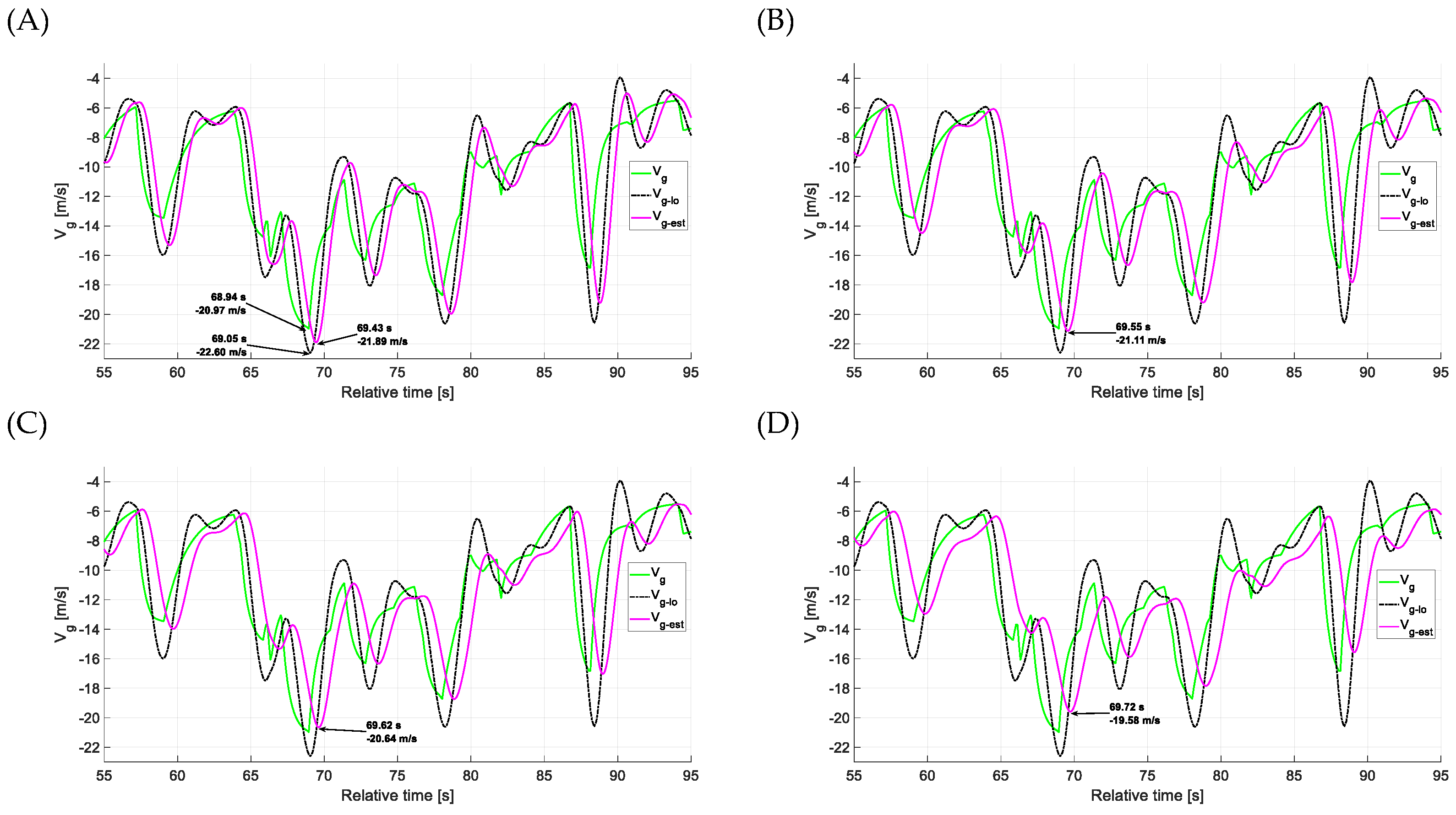
4.2. Estimation Accuracy—Side Gusts

The graphs in this section depict ideal side gusts measurement (obtained from the simulator’s weather section module) with the low-frequency signal Vg-lo (derived from speed and drift angle measurements) and the complete estimation Vg-est (a fusion of low-frequency signal Vg-lo and high frequency signal vg-hi—based on side acceleration measurement, using a CF). These comparisons were made for three considered phases of flight.
The first analyzed flight phase was descent (Figure 38, Figure 39 and Figure 40). Three data ranges were chosen for graphical presentation: the entire descent part of simulation (50–320 s), a series of selected gusts (120–195 s), and a single gust (146–168 s). The graphs illustrate the influence of varying the complementary filter time constant Tcv on the estimation results. Four selected time constant values {0.5 s, 0.8 s, 1 s, 1.5 s} were used for graphical comparison of the estimation against the recorded gusts.
Based on the charts, it can be concluded that the estimation results best matched the reference measurements for time constants of 0.5 s and 0.8 s. The assessment also confirmed that increasing the time constant from 0.8 s to 1.0 and 1.5 s led to an underestimation of the maximum gust values—mostly opposite to the trend observed in the head-on gusts estimation.
A detailed examination of the arrows marked with numerical values for the selected increasing gust in Figure 39 allows for a computational comparison. With a time constant of 0.5 s, the peak gust value in the full estimation is 1.01 m/s lower than the reference, while the low-frequency estimation shows a larger deviation of 1.83 m/s. The delay in the full estimation is 0.79 s, which is a deterioration over the 0.35-s delay observed in the low-frequency estimation. Increasing the time constant to 0.8 s allowed for an almost perfect match (0.11 m/s diffrence between the reference measurement) of the peak gust value considered while the full estimation delay increased to 0.93 s. Computational evaluation confirmed that increasing the time constant to 1.0 and 1.5 s resulted in an underestimation of the maximum gust values and increase in the delay to 1.1 s for Tcv = 1.5. Examining the numerical labels on the arrows in Figure 40 enables a precise comparison of the minimum values for the selected weakening gust scenario. With a time constant of 0.5 s, the minimum value differs by 0.68 m/s in the full estimation and by 1 m/s in the low-frequency estimation. The delay with respect to the reference measurement is only 0.03 s for the full estimation, and the low-frequency estimation is ahead of the baseline measurement by 0.35 s. When comparing the changes in the full estimated values for this selected case, the closest value of underestimation was achieved for a time constant of 1.0 s (0.2 m/s difference), with a relative small delay at the level of 0.33 s. A time constant of 1.5 s already overestimates the minimum value by 0.12 m/s, also increasing the estimation delay to 0.43 s.
For the considered cases, the best results were obtained for a time constant of 0.8 s for a gust with increasing velocity and for a time constant of 1.0 s for a gust with decreasing velocity. However, every increase in time constant in this algorithm for the level flight phase is associated with an increase in the delay of complete estimation, which is presented in detail in Table 3.
Afterward, the estimation results for the simulation conducted in level flight were presented. Three data ranges were selected for graphical analysis: the entire simulation (0–180 s), a series of selected gusts (50–85 s), and a single gust (60–74 s). The CF results reflect the impact of variations in the time constant Ts on the estimation result. For analysis, the same time constants were selected for comparison.
The evaluation based on charts presented in Figure 41, Figure 42 and Figure 43 leads to the conclusion that the best representation of the estimation results compared to the reference measurement was obtained for the time constant of 1.0 s. By examining the arrows annotated with numerical values for the selected rising gust speed in Figure 42, a computational comparison can be made. When using a time constant of 0.5 s, the differences between peak gust values are 2.54 m/s for complete estimation and 3.65 m/s for the low-frequency estimation with reference wind measurements. The full estimation shows a relatively small delay of 0.38 s compared to the reference, but no delay is observed in the low-frequency estimation. Raising the time constant to 0.8 s reduces the peak value of the overall estimation; however, the maximum value still surpasses the reference by 1.20 m/s. The delay also increases, going from 0.38 s to 0.56 s. When the time constant is further increased to 1.0 s, the estimation aligns most closely with the baseline in terms of the gust peak value, though the delay grows to 0.64 s. A final increase to a time constant of 1.5 s results in poorer numerical accuracy, leading to an underestimation. Reviewing the numerical labels on the arrows in Figure 43 enables a precise comparison of the minimum values for the selected decaying gust scenario. With a time constant of 0.5 s, the minimum value deviates by 2.85 m/s in the full estimation and by 3.93 m/s in the low-frequency estimation. The corresponding delays relative to the reference measurement are 0.5 s and 0.16 s, respectively. In this scenario, increasing the time constant results in progressively more accurate adjustments to the minimum value. The closest match to the reference measurement is observed at a time constant of 1.5 s, with a deviation of only 0.34 m/s. However, when considering the remaining gusts, their values are underestimated, indicating a general trend of underestimation. Thus, for both rising and falling gust conditions, the time constant of 1.0 s offers the most accurate velocity values. Nonetheless, this comes with an expected increase in delay, reaching approximately 0.65 s compared to shorter time constants.
The third case analyzed to evaluate the side gust estimation algorithm using complementary filtering involved climbing through a layer of head-on gusts. Three data ranges were selected for graphical presentation: the entire simulation (0–180 s), a series of selected gusts (55–95 s), and a single gust (65–80 s).
Data analysis (Figure 44, Figure 45 and Figure 46) shows that a time constant of 1.0 s provides the most accurate estimation results compared to the reference measurement. A numerical comparison, based on the arrows annotated with values for selected gusts in Figure 45 and Figure 46, supports this observation. Similar to the two earlier flight conditions, the optimal estimation for lateral gusts is achieved with a time constant of 1.0 s during rising gusts and 0.8 s during falling gusts. Increasing the time constant to 1.5 s leads to underestimation. Detailed computational results are provided in Table 3.
The side gust estimation results were evaluated by comparing them to the low-frequency signal in reference to the recorded ideal gusts measurements. Analysis of the graphs in the subection 4.2 indicates, that the applied estimation method allows for a more accurate representation of the gusts’ shape, and therefore their velocity, particularly in their extreme values, which pose the greatest threat to the aircraft. The estimation provides a more precise depiction of violent gusts where significant increases and decreases in gust speed occur over a short period of time, whereas the low-frequency signal tends to overestimate their magnitude. The undoubted advantage of the algorithm is its consistent performance across all evaluated flight conditions. Both the low-frequency signal and the estimation are delayed relative to the recorded side gusts. The best estimation is delayed by an average of 0.65 s. This delay is approximately 0.1 s longer than that observed in the estimation of head-on gusts. The low-frequency signal, although less accurate, reacted faster to the side gust—the delay in relation to the reference gusts was within 0.4–0.5 s. This is a faster response of the low-frequency signal compared to the estimation of head-on gusts. Furthermore, a higher value of the complementary filter time constant leads to a larger increase in the estimation delay in contrast to the head-on gust estimation algorithm. It would be necessary to define criteria for situations in which a shorter algorithm response time is preferable, even at the cost of underestimated peak values.
Table 3 summarizes the computational comparisons of the selected cases discussed above (the most favorable results are in bold). Negative values in the difference columns mean underestimation, and positive values mean overestimation.

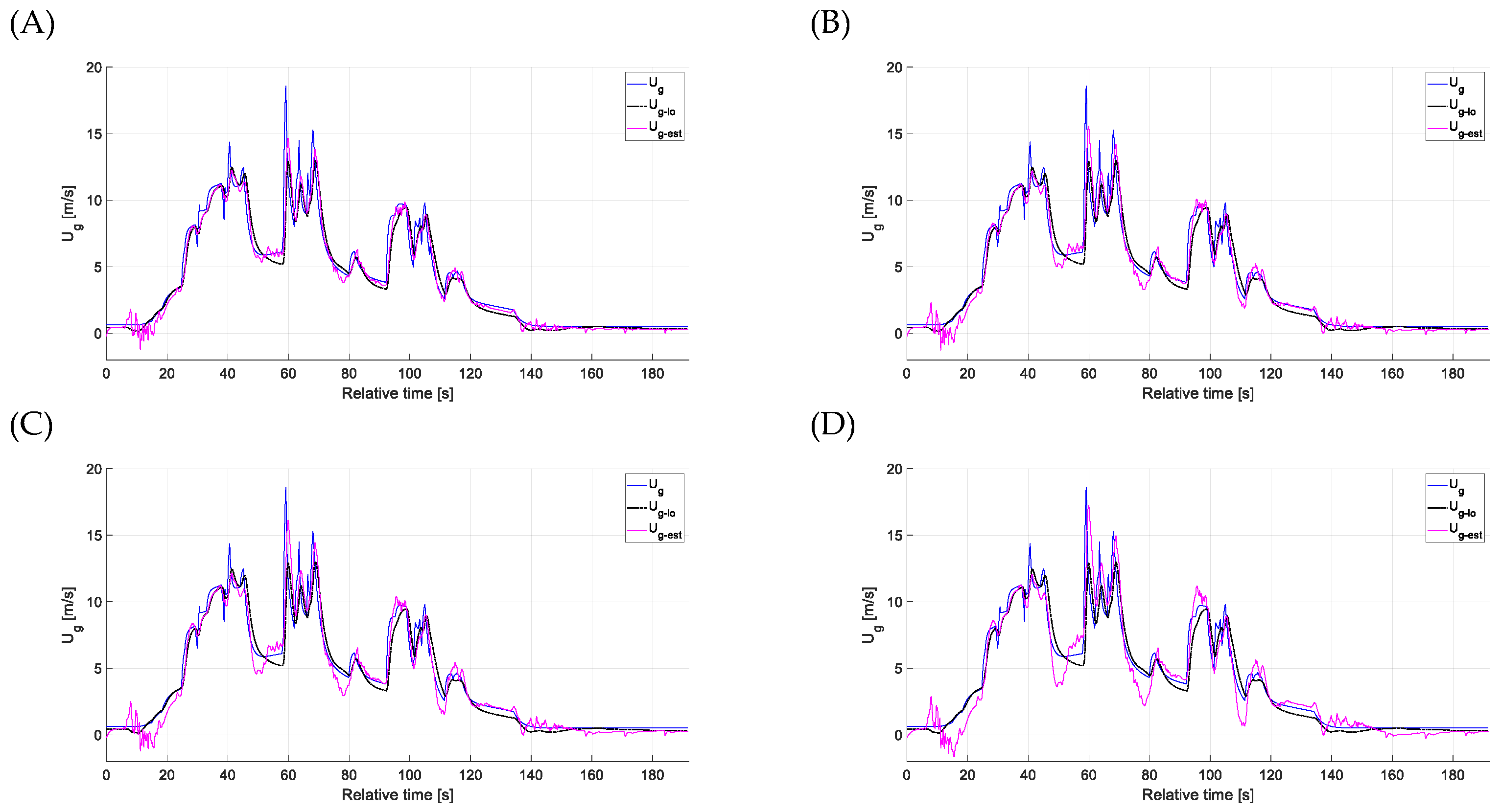
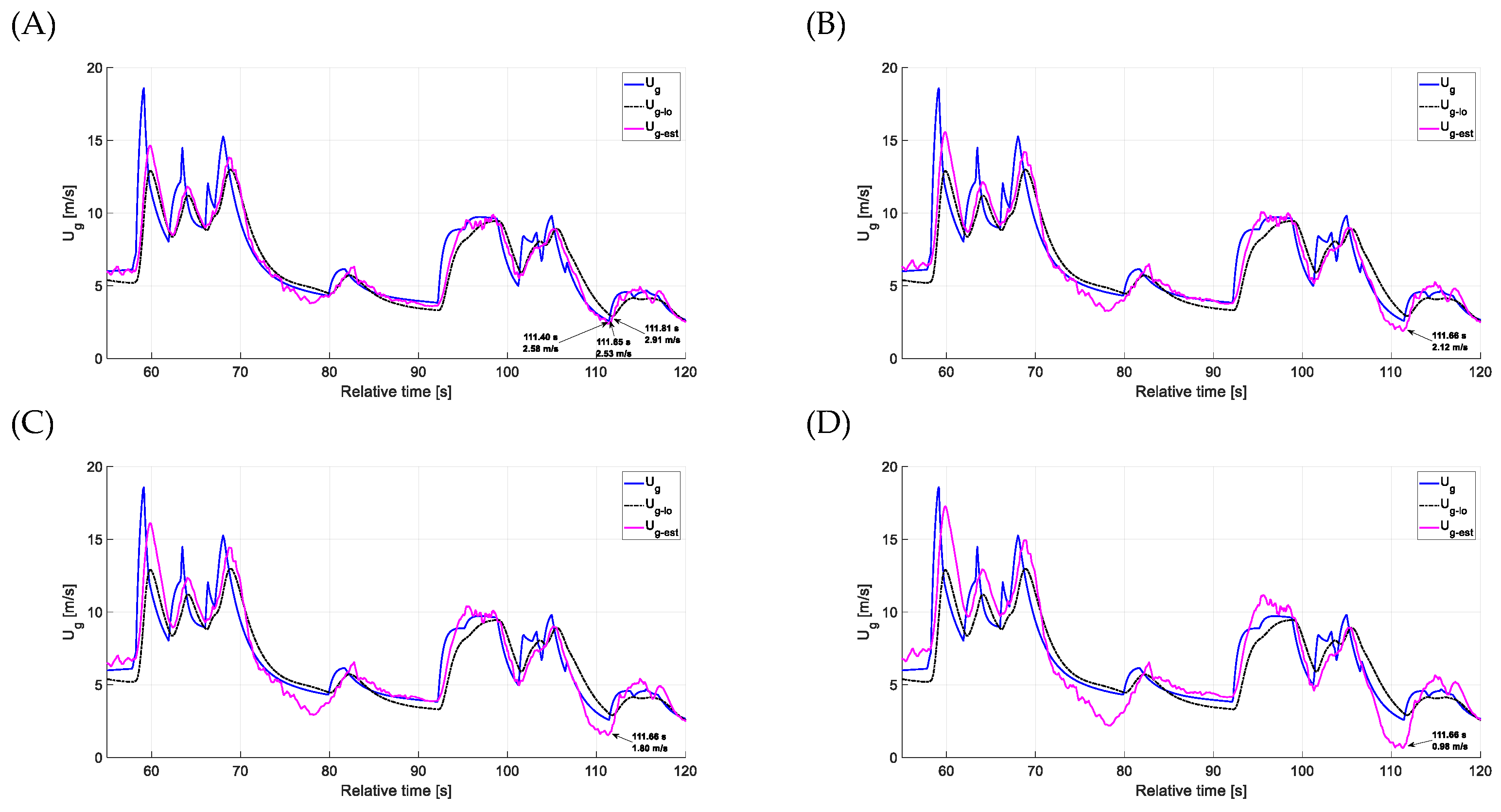
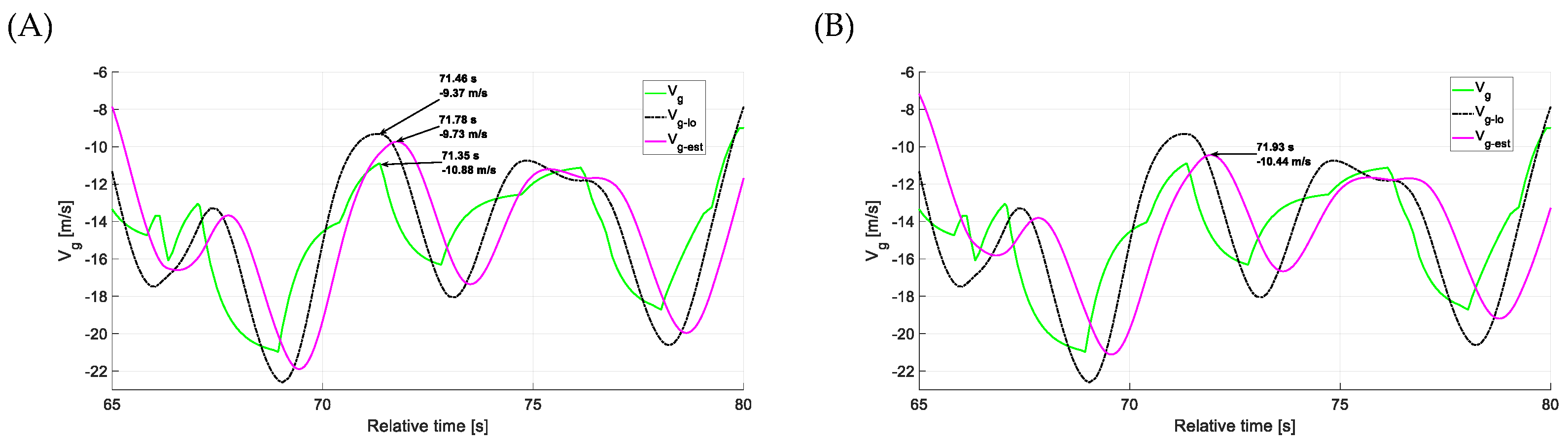
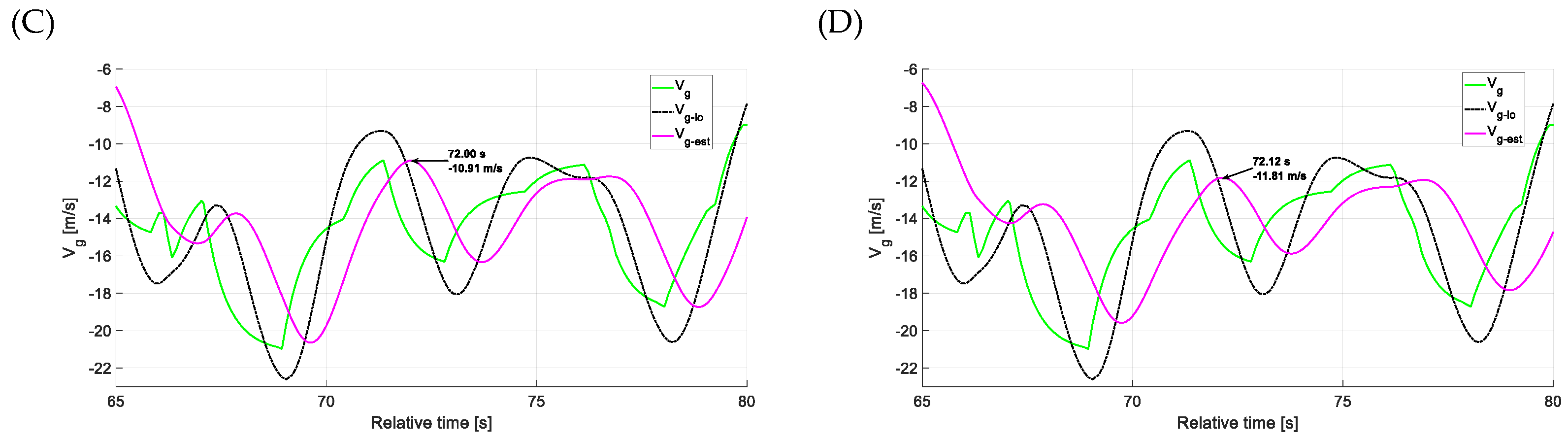
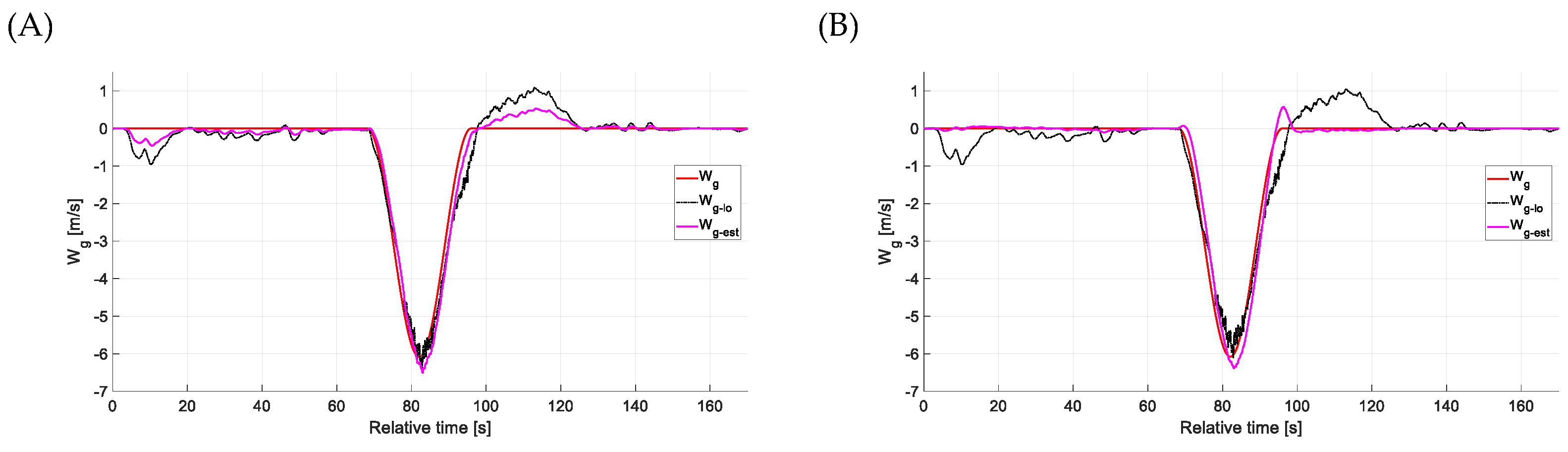
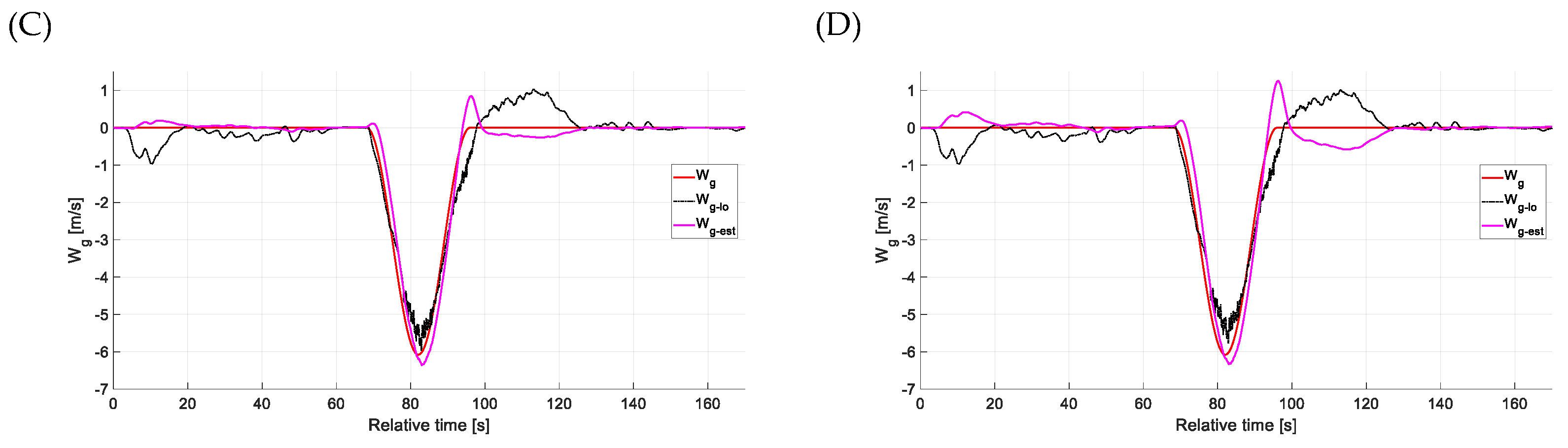
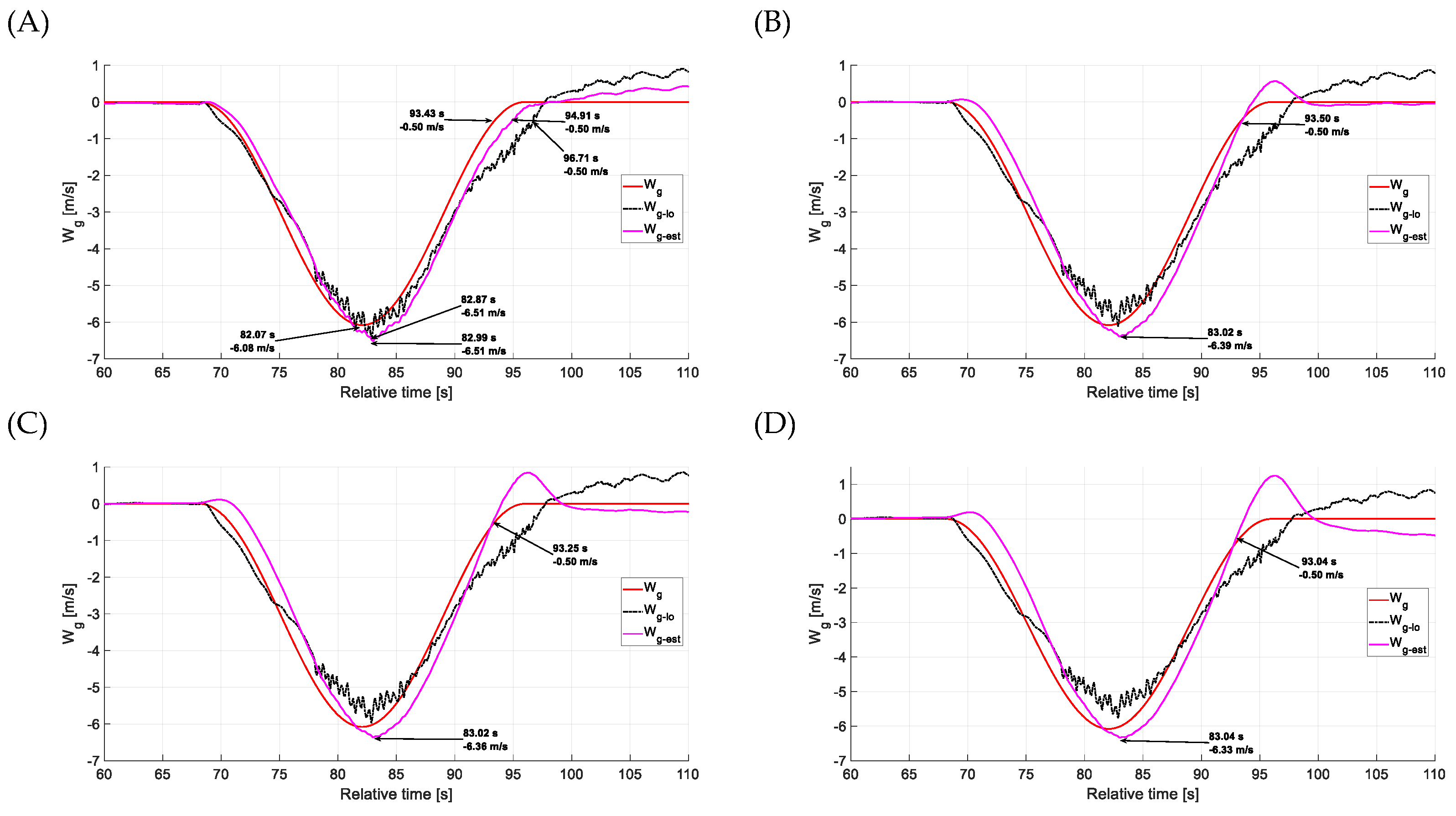
4.3. Estimation Accuracy—Vertical Gusts

The graphs in this section compare the ideal vertical gust measurements to the obtained low-frequency signal (Wg-lo) and the complete estimation (Wg-est), which combines the low-frequency signal (Wg-lo) and the high-frequency (wg-hi) signals using a CF across the three phases of flight. Based on the literature review, no direct method for determining vertical gusts using onboard systems in commercial aircraft has been identified. The developed low-frequency signals do not accurately represent the vertical gust value. Values comparable to the reference measurement can only be obtained after the fusion of the signals through additional filtering.
For the first analyzed flight phase—descent, two data ranges were selected for graphical presentation: the entire simulation (0–230 s) and a narrowed range during vertical gust occurrence (simulation time 100–140 s). The CF results illustrate the influence of varying the time constant Tcw on the estimation accuracy. Four time constant values {0.5 s, 1.0 s, 1.2 s, 1.5 s} were selected to account for the comparison of the estimation against the recorded gust.
Based on Figure 47 and Figure 48, it can be concluded that the estimation results most closely matched to the reference measurements for time constant of 1.2 s. In Figure 47, it is clearly shown that combining low- and high-frequency signals through complementary filtering greatly enhances the shape of the gust, specifically its velocity profile over time.
A closer examination of the arrows annotated with numerical data for the selected increasing gust in Figure 48 allows for a computational comparison. With a time constant of 0.5 s, there is a noticeable underestimation of the peak vertical gust velocity. Interestingly, the low-frequency and complete estimation signals initially lead the response, accurately capturing both the initial rise in gust velocity and the peak value. However, the accuracy deteriorates as the gust velocity returns to zero. To quantify the delay in reverting to pre-gust conditions, a reference point at a velocity of −0.5 m/s was chosen for each signal analyzed. Despite initially leading the reference measurement, the signals exhibit a substantial lag—exceeding 3 s—at this point. The increase in time constants to 1.0 s and 1.2 s brings the peak value of the estimated vertical gust closer to the reference value at the cost of increasing the delay. However, there is an improvement due to the decrease in delay for decreasing the gust speed. Detailed comparative data are presented in Table 4. Data analysis allows a less precise return of the full estimate to zero after the gust has subsided. This issue becomes more pronounced with a time constant of 1.5 s, where the peak is also overestimated. Overall, it is important to note that the average delay is greater compared to the other two algorithms, reaching around 1.5 s during the descent phase of flight.
Subsequently, the estimation results for the simulation conducted in level flight were presented. Two data ranges were selected for graphical analysis: the entire simulation (0–100 s) and the narrowed range during vertical gust occurrence (simulation time 45–75 s). The CF results reflect the influence of varying the time constant Tcw on the estimation performance. For analysis, the same time constants were selected for comparison.
Data analysis based on Figure 49 and Figure 50 indicates that time constants of 0.5 s and 1.0 s provided the closest match between the estimated results and the reference measurement.
A detailed look at the arrows annotated with numerical data for the selected increasing gust in Figure 50 enables a computational comparison. With a time constant of 0.5 s, the estimated peak vertical gust differs from the reference by only 0.05 m/s, with a delay of 0.56 s. However, this time constant also results in a delay of 1.74 s for reaching a velocity of 0.5 m/s during the gust’s decline. Figure 50 indicates a notably accurate return to zero after the vertical gust ends when using a time constant of 1.0 s, with an average overall delay of 0.975 s. In comparison, the other time constants analyzed perform less favorably in this aspect. According to Table 4, increasing the time constant further to 1.2 s and 1.5 s does not significantly affect the total delay, which remains approximately 0.5 s shorter than in the previously examined descent flight phase.
The third scenario analyzed to evaluate the vertical gust estimation algorithm using complementary filtering involved flying through a microburst during climb. Two data ranges were selected for graphical presentation: the entire simulation (0–170 s) and the narrowed range of vertical gust occurrence (simulation time 60–110 s).
Figure 51 and Figure 52 demonstrate that a time constant of 1.0 s yields the most accurate estimation results relative to the reference measurement. Significant differences are observed in the return to zero values following the vertical gust, with the most favorable outcome occurring at a time constant of 1.0 s.
In contrast to the two previously analyzed flight conditions, the peak values of the vertical gust are overestimated during the climb phase. Increasing the time constant reduces the discrepancy between the estimated and reference values, although, as indicated in Table 4, these differences remain relatively minor. For the weakening phase of the gust—specifically at the −0.5 m/s velocity point—raising the time constant from 0.5 s to 1.0 s significantly reduced the estimation delay from 1.48 s to just 0.07 s. For this criterion, further increasing the time constants causes the estimation to be too far ahead of the reference measurement. However, further increases in the time constant lead to the estimation anticipating the reference measurement, while at the same time causing problems with stabilizing the zero values after the vertical gust has subsided.
The vertical gust estimation results were evaluated by comparing them to the low-frequency signal and the recorded ideal gusts measurements. Analysis of the graphs from Section 4.3, indicates that the applied estimation method provides a more accurate representation of the gusts’ shape, and therefore their velocity, than the low-frequency signal alone. The estimation more accurately captured the decrease in gust velocity, whereas the low-frequency signal exceeded the reference signal during this phase. The whole simulation graphs showed that, in the case of estimation, there was a quicker return to zero after the gust subsided, compared to the low-frequency signal, especially for a time constant equal to 1.0 s. The vertical gust estimation algorithm is less predictable compared to the developed head-on and side gusts estimation algorithms. Interestingly, the low-frequency signal slightly preceded the reference gust during its initial phase. The estimation is delayed by an average of 1.0 s for the level flight and climb phases and by an average of 1.5 s for the descent phase, relative to the recorded reference gust for the most accurate results in terms of value. Furthermore, a higher value of the complementary filter time constant leads to difficulties in maintaining stable zero values after the vertical gust has diminished. In the analyzed vertical gust scenario, the potential impact of a simultaneously occurring strong headwind gust and a minor crosswind component on the estimation results was considered. In the contrast, for the previously analyzed separated head-on and side gusts scenarios (Section 4.1 and Section 4.2), the influence of other wind components was eliminated by carefully selecting the simulation conditions.
Table 4 summarizes the computational comparisons of the selected cases discussed above (the most favorable results are in bold). Negative values in the difference columns mean underestimation, and positive values mean overestimation. When interpreting the average deceleration values from Table 4, the negative values of the last two time constants for the climb case must be taken into account, which lower these average results.

5. Conclusions

For CS-25 EASA category aircraft, most of which are characterized by a relatively high mass, resistance to small gusts is generally high. However, in the presence of more significant disturbances, such as those caused by wind shear, recovery—particularly during the terminal phases of flight—can be challenging. In such scenarios, early gust detection systems are crucial, as they support rapid decision-making and accurate identification of the phenomena, thereby reducing susceptibility to human error.
When deriving the dependencies enabling gust estimation, dynamics models, including control system interactions, were employed. However, the final results, expressed in formulas (32), (38), and (42), are independent of specific flight states, and thus remain unaffected by the particularities of the aircraft dynamics model. In our previous study [30], we partially applied flight-state-sensitive estimation. In the present manuscript, we demonstrate that this issue can be circumvented without any significant impact on the practical results. We consider this to be one of the key advantages of the proposed solution.
The developed estimation algorithms enable relatively fast and accurate determination of atmospheric gust parameters. The results obtained confirm their reliable performance under various flight conditions. In summary, the average estimation delay ranged from 0.4 to 0.67 s for the head-on gust estimation algorithm, from 0.50 to 0.67 s for the side gust estimation algorithm, and from 0.91 to 1.6 s for the vertical gust estimation algorithm, depending on the selected time constant. The selection of time constants for evaluating the accuracy of different gust types was guided by the following criteria: first, alignment of the estimation results with reference measurements in terms of gust waveform shape and peak values; second, achieving the lowest possible estimation delay relative to the reference data; and third, improvement in the representation of low-frequency signal components. In further work on the developed algorithms, it is essential to establish clear criteria and a structured methodology for accurately determining the optimal time constant for each algorithm and, ultimately, for each flight phase. Additionally, guidelines should be defined for situations where a faster algorithm response is prioritized, even at the cost of underestimating peak values.
It is important to note that the simulation environment may affect the accuracy of the results when compared to real flight tests. The dynamic behavior of the aircraft in the simulator may differ from that of the actual aircraft. However, the simulation environment enables comparisons of algorithms with a reference measurements, which is challenging to accomplish during real flight tests. It would be beneficial to validate the developed algorithms using data from a certified Class D FFS simulator, although recording such data remains difficult due to manufacturer restrictions.
A practical application of the discussed estimation algorithms could involve their integration into a cockpit indication system for flight crews. Enhanced three-dimensional gust data could be presented either via a dedicated visual display (e.g., an axonometric projection), incorporated into the Primary Flight Display (PFD) or Multi-Function Display (MFD). In addition to visual cues, the system could also incorporate audible alerts. Another potential application is the transmission of complete or selected critical measurement data between aircraft conducting similar operations in close succession, or to air traffic control services—using systems such as the Aircraft Communications Addressing and Reporting System (ACARS) or Controller Pilot Data Link Communications (CPDLC).

Author Contributions

Conceptualization, P.S. and P.R.; methodology, P.S., P.R. and P.G.; software, P.S., P.R., P.G. and K.W.; validation, P.S., P.R. and P.G.; formal analysis, P.S., P.R. and P.G.; investigation, P.S., P.R., P.G. and K.W.; resources, P.S. and P.R.; data curation, P.S. and P.R.; writing—original draft preparation, P.S., P.R., P.G. and K.W.; writing—review and editing, P.S., P.R., P.G. and K.W.; visualization, P.S., P.R. and P.G.; supervision, P.R. and P.G.; project administration, P.S., P.R. and P.G.; funding acquisition, P.R. All authors have read and agreed to the published version of the manuscript.

Funding

This research received no external funding.

Informed Consent Statement

Not applicable.

Data Availability Statement

The data presented in this study are available on request from the corresponding author.

Conflicts of Interest

The authors declare no conflicts of interest.

References

  1. ICAO. Manual on Low-Level Wind Shear; Doc 9817 AN/449; International Civil Aviation Organization: Montréal, QC, Canada, 2005; ISBN 92-9194-609-5. [Google Scholar]
  2. FAA. Windshear Weather. In Wind Shear Training Aid; Federal Aviation Authority: Washington, DC, USA, 1990; Volume 2, pp. 4.2-1–4.2-133. [Google Scholar]
  3. Krusiec, G. On-Board Wind Shear Warning System; Rzeszów University of Technology: Rzeszów, Poland, 2010. [Google Scholar]
  4. O’Connor, A. Demonstration of a Novel 3-D Wind Sensor for Improved Wind Shear Detection for Aviation Operations. Master’s Thesis, Technological University Dublin, Dublin, Ireland, 2018. [Google Scholar] [CrossRef]
  5. O’Connor, A. Using a Wind Urchin for Airport Wind Measurements, Retrieved from Irish Meteorological Society. Master’s Thesis, Technological University Dublin, Dublin, Ireland, 2018. [Google Scholar]
  6. Brandl, A.; Battipede, M. Maneuver-Based Cross-Validation Approach for Angle-of-Attack Estimation. In Proceedings of the 14th WCCM-ECCOMAS Congress, Virtual, 11–15 January 2020; Volume 1700. [Google Scholar]
  7. The Aviation Herald. Incidents and News in Aviation. Available online: www.avherald.com (accessed on 8 May 2025).
  8. Kelley, N.D.; Jonkman, B.J.; Scott, G.N. Comparing Pulsed Doppler LIDAR with SODAR and Direct Measurements for Wind Assessment. In Proceedings of the American Wind Energy Association WindPower 2007 Conference and Exhibition, Los Angeles, CA, USA, 3–7 June 2007; National Renewable Energy Laboratory: Golden, CO, USA, 2007. [Google Scholar]
  9. Fezans, N.; Joos, H.-D.; Deiler, C. Gust load alleviation for a long-range aircraft with and without anticipation. CEAS Aeronaut. J. 2019, 10, 1033–1057. [Google Scholar] [CrossRef]
  10. Prudden, S.; Fisher, A.; Marino, M.; Mohamed, A.; Watkins, S.; Wild, G. Measuring wind with small unmanned aircraft systems. J. Wind. Eng. Ind. Aerodyn. 2018, 176, 197–210. [Google Scholar] [CrossRef]
  11. Ellrod, G.P.; Knapp, D.I. An objective clear-air turbulence forecasting technique: Verification and operational use. Weather. Forecast 1992, 7, 150–165. [Google Scholar] [CrossRef]
  12. Di Vito, V.; Zollo, A.L.; Cerasuolo, G.; Montesarchio, M.; Bucchignani, E. Clear Air Turbulence and Aviation Operations: A Literature Review. Sustainability 2025, 17, 4065. [Google Scholar] [CrossRef]
  13. Prosser, M.C.; Williams, P.D.; Marlton, G.J.; Harrison, R.G. Giles Harrison. Evidence for Large Increases in Clear-Air Turbulence Over the Past Four Decades. Geophys. Res. Lett. 2023, 50, e2023GL103814. [Google Scholar] [CrossRef]
  14. Forester, J. What You Need to Know about Clear Air Turbulence. Forbes, Innovation Science. Available online: https://www.forbes.com/sites/jimfoerster/2024/05/24/what-you-need-to-know-about-clear-air-turbulence/ (accessed on 28 May 2024).
  15. Arranz, A.; Kawoosa, V.M.; Kiyada, S.; Huang, H.; Zafra, M.; Scarr, S. The Mechanics of Turbulence. Thomson Reuters Group Limited. Available online: https://www.reuters.com/graphics/SINGAPOREAIRLINES-THAILAND/movaqnmeava/ (accessed on 22 May 2024).
  16. Wong, C. Singapore Airlines turbulence: Why climate change is making flights rougher. Nature 2024. [Google Scholar] [CrossRef]
  17. IATA. Findings and Conclusions. In Proceedings of the Go-around Safety Forum, Brussels, Belgium, 18 June 2013; International Air Transport Association: Singapore, 2013. [Google Scholar]
  18. Tomczyk, A. Zastosowanie Analitycznej Redundancji Pomiarów w Układzie Sterowania i Nawigacji Statku Powietrznego (Application of Analytical Redundancy of Measurements in Aircraft Control and Navigation System). In Proceedings of the Scientific Aspects Concerning Operation of Manned and Unmanned Aerial Vehicles, Dęblin, Poland, 15–17 May 2015. [Google Scholar]
  19. Hamke, E.E.; Enns, D.F.; Loe, G.R.; Wacker, R.A.; Schubert, O. Wind Estimation for an Unmanned Aerial Vehicle. U.S. Patent US8219267B2, 10 July 2012. [Google Scholar]
  20. Hall, A.P.; Marton, T.F.; Muren, P. Passive Local Wind Estimator. U.S. Patent US20140129057A1, 8 May 2014. [Google Scholar]
  21. Hall, A.P.; Marton, T.F.; Muren, P. Passive Local Wind Estimator. U.S. Patent US9031719B2, 12 May 2015. [Google Scholar]
  22. Kumon, M.; Mizumoto, I.; Iwai, Z.; Nagata, M. Wind estimation by unmanned air vehicle with delta wing. In Proceedings of the 2005 IEEE International Conference on Robotics and Automation, Barcelona, Spain, 18–22 April 2005; IEEE: Piscataway, NJ, USA, 2005; pp. 1896–1901. [Google Scholar]
  23. Meier, K.; Hann, R.; Skaloud, J.; Garreau, A. Wind Estimation with Multirotor UAVs. Atmosphere 2022, 13, 551. [Google Scholar] [CrossRef]
  24. Frant, M.; Kachel, S.; Maślanka, W. Gust Modeling with State-of-the-Art Computational Fluid Dynamics (CFD) Software and Its Influence on the Aerodynamic Characteristics of an Unmanned Aerial Vehicle. Energies 2023, 16, 6847. [Google Scholar] [CrossRef]
  25. Reuder, J.; Jonassen, M.O.; Ólafsson, H. The Small Unmanned Meteorological Observer SUMO: Recent developments and applications of a micro-UAS for atmospheric boundary layer research. Acta Geophys. 2012, 60, 1454–1473. [Google Scholar] [CrossRef]
  26. Brezoescu, A.; Castillo, P.; Lozano, R. Wind estimation for accurate airplane path following applications. J. Intell. Robot. Syst. 2014, 73, 823–831. [Google Scholar] [CrossRef]
  27. Wingrove, R.C.; Bach, R.E., Jr. Severe turbulence and maneuvering from airline flight records. J. Aircr. 1994, 31, 753–760. [Google Scholar] [CrossRef]
  28. Szwed, P.; Rzucidło, P.; Rogalski, T. Estimation of Atmospheric Gusts Using Integrated On-Board Systems of a Jet Transport Airplane—Flight Simulations. Appl. Sci. 2022, 12, 6349. [Google Scholar] [CrossRef]
  29. Bociek, S.; Gruszecki, J. Automatic Aircraft Control Systems; Oficyna wydawnicza Politechniki Rzeszowskiej: Rzeszów, Poland, 1999. (In Polish) [Google Scholar]
  30. Cook, M.V. Flight Dynamic Principal; Elsevier: Burlington, MA, USA, 2007; pp. 1–401. [Google Scholar]
  31. Grzybowski, P.; Klimczuk, M.; Rzucidlo, P. Distributed Measurement System Based on CAN Data Bus. Aircr. Eng. Aerosp. Technol. 2018, 90, 1249–1258. [Google Scholar] [CrossRef]
  32. Welcer, M.; Szczepański, C.; Krawczyk, M. The Impact of Sensor Errors on Flight Stability. Aerospace 2022, 9, 169. [Google Scholar] [CrossRef]
  33. Dołęga, B.; Kopecki, G.; Tomczyk, A. Analytical redundancy in control systems for unmanned aircraft and optionally piloted vehicles. Trans. Aerosp. Res. 2017, 2017, 31–44. [Google Scholar] [CrossRef]
  34. Kopecki, G.; Tomczyk, A.; Rzucidło, P. Algorithms of measurement system for a micro UAV. Solid State Phenom. 2013, 198, 165–170. [Google Scholar] [CrossRef]
  35. Dąbrowski, W.; Popowski, S. Estimation of wind parameters on flying objects. Pomiary Autom. Robot. 2013, 17, 552–557. [Google Scholar]
  36. Rautenberg, A.; Graf, M.S.; Wildmann, N.; Platis, A.; Bange, J. Reviewing Wind Measurement Approaches for Fixed-Wing Unmanned Aircraft. Atmosphere 2018, 9, 422. [Google Scholar] [CrossRef]
  37. Narkhede, P.; Poddar, S.; Walambe, R.; Ghinea, G.; Kotecha, K. Cascaded Complementary Filter Architecture for Sensor Fusion in Attitude Estimation. Sensors 2021, 21, 1937. [Google Scholar] [CrossRef]
  38. Lerro, A.; Brandl, A.; Gili, P. Model-free scheme for angle-of-attack and angle-of-sideslip estimation. J. Guid. Control. Dyn. 2021, 44, 595–600. [Google Scholar] [CrossRef]
  39. Baldwin, W.A. Method for Determining Airplane Flight-Path Angle with the Use of Airspeed and the Global Positioning System (GPS). U.S. Patent No 10,823,752, 3 November 2020. [Google Scholar]
  40. Mulder, J.A.; Chu, Q.P.; Sridhar, J.K.; Breeman, J.H.; Laban, M. Non-linear aircraft flight path reconstruction review and new advances. Prog. Aerosp. Sci. 1999, 35, 673–726. [Google Scholar] [CrossRef]
  41. X-Plane Communication Toolbox (XPC). Available online: https://software.nasa.gov/software/ARC-17185-1 (accessed on 24 February 2024).
  42. Welcer, M.; Sahbon, N.; Zajdel, A. Comparison of Flight Parameters in SIL Simulation Using Commercial Autopilots and X-Plane Simulator for Multi-Rotor Models. Aerospace 2024, 11, 205. [Google Scholar] [CrossRef]
  43. Yu, L.; He, G.; Zhao, S.; Wang, X.; Shen, L. Design and Implementation of a Hardware-in-the-Loop Simulation System for a Tilt Trirotor UAV. J. Adv. Transp. 2020, 2020, 4305742. [Google Scholar] [CrossRef]
  44. Bittar, A.; Figuereido, H.V.; Guimaraes, P.A.; Mendes, A.C. Guidance software-in-the-loop simulation using x-plane and simulink for UAVs. In Proceedings of the 2014 International Conference on Unmanned Aircraft Systems (ICUAS), Orlando, FL, USA, 27–30 May 2014; IEEE: Piscataway, NJ, USA; pp. 993–1002. [Google Scholar]
  45. Brady, C. The Boeing 737 Technical Guide; Lightning Source: Milton Keynes, UK, 2018. [Google Scholar]
  46. Goff, R.C. The Low-Level Wind Shear Alert System Report; Final Report for U.S. Department of Transportation; National Aviation Facilities Experimental Center: Washington, DC, USA, 1980. [Google Scholar]
  47. Obserwator. Dangerous Atmospheric Phenomena in Aviation: Wind and Turbulence. Available online: https://obserwator.imgw.pl/2020/07/30/dangerous-atmospheric-phenomena-in-aviation-wind-and-turbulence/ (accessed on 8 May 2025).
  48. Klug, L.; Ullah, J.; Lutz, T.; Streit, T.; Heinrich, R.; Radespiel, R. Gust alleviation by spanwise load control applied on a forward and backward swept wing. CEAS Aeronaut. J. 2023, 14, 435–454. [Google Scholar] [CrossRef]
  49. Ullah, J.; Kamoun, S.; Müller, J.; Lutz, T. Active gust load alleviation by means of steady and dynamic trailing and leading edge flap deflections at transonic speeds. In Proceedings of the AIAA SCITECH 2022 Forum, San Diego, CA, USA, 3–7 January 2022; p. 1334. [Google Scholar]
Figure 1. Illustration of a flight through the microburst phenomenon. (A)—increase in headwind speed; indicated air speed increases, rate of descent decreases, tendency to go above the assumed glide path. (B)—decrease in headwind speed; downdraft increases, indicated airspeed decreases, rate of descent increases, tendency to descend below the assumed glide path. (C)—increase in tailwind speed; the indicated air speed is constantly decreasing, the approach is interrupted at decision height, success depends on altitude, current speed and power reserve.
Applsci 15 05687 g001
Figure 2. Illustration of relations from Equation (27).
Applsci 15 05687 g002
Figure 3. Diagram of complementary filter.
Applsci 15 05687 g003
Figure 4. Bode diagram (amplitude and phase) for linear CF.
Applsci 15 05687 g004
Figure 5. Illustration of relations from Equation (27).
Applsci 15 05687 g005
Figure 6. Illustration of relations from Equation (39).
Applsci 15 05687 g006
Figure 7. Stationary simulator stand with cockpit view of a jet airliner—Boeing 737-800.
Applsci 15 05687 g007
Figure 8. Block diagram of the simulator station and data acquisition.
Applsci 15 05687 g008
Figure 9. External view of a Boeing 737-800 during simulation (X-Plane v11 Pro, B737-800 ZIBO model).
Applsci 15 05687 g009
Figure 10. Coordinate systems: OpenGL—related to the Earth (red), fixed to the center of gravity of the aircraft (green), related to the plane (blue).
Applsci 15 05687 g010
Figure 11. (A) Altitude, (B) IAS, and (C) VVI recorded during simulated flight—descent phase.
Applsci 15 05687 g011
Figure 12. Registered ideal gust measurements from simulation weather section—descent phase; (A)—wind speed as a function of time, (B)—wind speed as a function of altitude.
Applsci 15 05687 g012
Figure 13. (A) Altitude, (B) IAS, and (C) VVI recorded during simulated level flight.
Applsci 15 05687 g013
Figure 14. Registered ideal gust measurements from simulation weather section—level flight; wind speed as a function of time.
Applsci 15 05687 g014
Figure 15. (A) Altitude, (B) IAS, and (C) VVI recorded during simulated flight—climb phase.
Applsci 15 05687 g015
Figure 16. Registered ideal gusts measurements from the simulation weather section—climb phase; (A)—wind speed as a function of time, (B)—wind speed as a function of altitude.
Applsci 15 05687 g016
Figure 17. (A) Altitude, (B) IAS, and (C) VVI recorded during simulated flight—descent phase.
Applsci 15 05687 g017
Figure 18. Registered ideal gusts measurements from the simulation weather section—descent phase; (A)—wind speed as a function of time, (B)—wind speed as a function of altitude.
Applsci 15 05687 g018
Figure 19. (A) Altitude, (B) IAS, and (C) VVI recorded during simulated level flight.
Applsci 15 05687 g019
Figure 20. Registered ideal gusts measurements from the simulation weather section—level flight; wind speed as a function of time.
Applsci 15 05687 g020
Figure 21. (A) Altitude, (B) IAS, and (C) VVI recorded during simulated flight—climb phase.
Applsci 15 05687 g021
Figure 22. Registered ideal gusts measurements from the simulation weather section—climb phase; (A)—wind speed as a function of time, (B)—wind speed as a function of altitude.
Applsci 15 05687 g022
Figure 23. (A) Altitude, (B) IAS, and (C) VVI recorded during simulated flight—descent phase.
Applsci 15 05687 g023
Figure 24. Registered ideal gusts measurements from the simulation weather section—descent phase; (A)—wind speed as a function of time, (B)—wind speed as a function of altitude.
Applsci 15 05687 g024
Figure 25. (A) Altitude, (B) IAS, and (C) VVI recorded during simulated level flight.
Applsci 15 05687 g025
Figure 26. Registered ideal gusts measurements from the simulation weather section—level flight; wind speed as a function of time.
Applsci 15 05687 g026
Figure 27. (A) Altitude, (B) IAS, and (C) VVI recorded during simulated flight—climb phase.
Applsci 15 05687 g027
Figure 28. Registered ideal gusts measurements from the simulation weather section—climb phase; (A)—wind speed as a function of time, (B)—wind speed as a function of altitude.
Applsci 15 05687 g028
Figure 29. Comparison of the gust value with the estimation results—descent crossing a gust area; entire simulation (complementary filter, (A) Tcu = 0.5 s, (B) Tcu = 0.8 s, (C) Tcu = 1.0 s, (D) Tcu = 1.5 s).
Applsci 15 05687 g029
Figure 30. Comparison of the gust value with the estimation results—descent crossing a gust area; series of selected gusts (complementary filter, (A) Tcu = 0.5 s, (B) Tcu = 0.8 s, (C) Tcu = 1.0 s, (D) Tcu = 1.5 s).
Applsci 15 05687 g030
Figure 31. Comparison of the gust value with the estimation results—descent crossing a gust area; single selected gust (complementary filter, (A) Tcu = 0.5 s, (B) Tcu = 0.8 s, (C) Tcu = 1.0 s, (D) Tcu = 1.5 s).
Applsci 15 05687 g031
Figure 32. Comparison of the gust value with the estimation results—level flight through a gust area; entire simulation (complementary filter, (A) Tcu = 0.5 s, (B) Tcu = 0.8 s, (C) Tcu = 1.0 s, (D) Tcu = 1.5 s).
Applsci 15 05687 g032
Figure 33. Comparison of the gust value with the estimation results—level flight through a gust area; series of selected gusts (complementary filter, (A) Tcu = 0.5 s, (B) Tcu = 0.8 s, (C) Tcu = 1.0 s, (D) Tcu = 1.5 s).
Applsci 15 05687 g033
Figure 34. Comparison of the gust value with the estimation results—level flight through a gust area; single selected gust (complementary filter, (A) Tcu = 0.5 s, (B) Tcu = 0.8 s, (C) Tcu = 1.0 s, (D) Tcu = 1.5 s).
Applsci 15 05687 g034
Figure 35. Comparison of the gust value with the estimation results—climb crossing a gust area; entire simulation (complementary filter, (A) Tcu = 0.5 s, (B) Tcu = 0.8 s, (C) Tcu = 1.0 s, (D) Tcu = 1.5 s).
Applsci 15 05687 g035
Figure 36. Comparison of the gust value with the estimation results—climb crossing a gust area; series of selected gusts (complementary filter, (A) Tcu = 0.5 s, (B) Tcu = 0.8 s, (C) Tcu = 1.0 s, (D) Tcu = 1.5 s).
Applsci 15 05687 g036
Figure 37. Comparison of the gust value with the estimation results—climb crossing a gust area; single selected gust (complementary filter, (A) Tcu = 0.5 s, (B) Tcu = 0.8 s, (C) Tcu = 1.0 s, (D) Tcu = 1.5 s).
Applsci 15 05687 g037
Figure 38. Comparison of the gust value with the estimation results—descent crossing a gust area; entire descent part of simulation (complementary filter, (A) Tcv = 0.5 s, (B) Tcv = 0.8 s, (C) Tcv = 1.0 s, (D) Tcv = 1.5 s).
Applsci 15 05687 g038
Figure 39. Comparison of the gust value with the estimation results—descent crossing a gust area; series of selected gusts (complementary filter, (A) Tcv = 0.5 s, (B) Tcv = 0.8 s, (C) Tcv = 1.0 s, (D) Tcv = 1.5 s).
Applsci 15 05687 g039
Figure 40. Comparison of the gust value with the estimation results—descent crossing a gust area; single selected gust (complementary filter, (A) Tcv = 0.5 s, (B) Tcv = 0.8 s, (C) Tcv = 1.0 s, (D) Tcv = 1.5 s).
Applsci 15 05687 g040
Figure 41. Comparison of the gust value with the estimation results—level flight through a gust area; entire simulation (complementary filter, (A) Tcv = 0.5 s, (B) Tcv = 0.8 s, (C) Tcv = 1.0 s, (D) Tcv = 1.5 s).
Applsci 15 05687 g041
Figure 42. Comparison of the gust value with the estimation results—level flight through a gust area; series of selected gusts (complementary filter, (A) Tcv = 0.5 s, (B) Tcv = 0.8 s, (C) Tcv = 1.0 s, (D) Tcv = 1.5 s).
Applsci 15 05687 g042
Figure 43. Comparison of the gust value with the estimation results—level flight through a gust area; single selected gust (complementary filter, (A) Tcv = 0.5 s, (B) Tcv = 0.8 s, (C) Tcv = 1.0 s, (D) Tcv = 1.5 s).
Applsci 15 05687 g043
Figure 44. Comparison of the gust value with the estimation results—climb crossing a gust area; entire simulation (complementary filter, (A) Tcv = 0.5 s, (B) Tcv = 0.8 s, (C) Tcv = 1.0 s, (D) Tcv = 1.5 s).
Applsci 15 05687 g044
Figure 45. Comparison of the gust value with the estimation results—climb crossing a gust area; series of selected gusts (complementary filter, (A) Tcv = 0.5 s, (B) Tcv = 0.8 s, (C) Tcv = 1.0 s, (D) Tcv = 1.5 s).
Applsci 15 05687 g045
Figure 46. Comparison of the gust value with the estimation results—climb crossing a gust area; single selected gust (complementary filter, (A) Tcv = 0.5 s, (B) Tcv = 0.8 s, (C) Tcv = 1.0 s, (D) Tcv = 1.5 s).
Applsci 15 05687 g046aApplsci 15 05687 g046b
Figure 47. Comparison of the gust value with the estimation results—descent crossing a microburst; entire simulation (complementary filter, (A) Tcw = 0.5 s, (B) Tcw = 1.0 s, (C) Tcw = 1.2 s, (D) Tcw = 1.5 s).
Applsci 15 05687 g047
Figure 48. Comparison of the gust value with the estimation results—descent crossing a microburst; single vertical gust (complementary filter, (A) Tcw = 0.5 s, (B) Tcw = 1.0 s, (C) Tcw = 1.2 s, (D) Tcw = 1.5 s).
Applsci 15 05687 g048aApplsci 15 05687 g048b
Figure 49. Comparison of the gust value with the estimation results—microburst during a level flight; entire simulation (complementary filter, (A) Tcw = 0.5 s, (B) Tcw = 1.0 s, (C) Tcw = 1.2 s, (D) Tcw = 1.5 s).
Applsci 15 05687 g049
Figure 50. Comparison of the gust value with the estimation results—microburst during a level flight; single vertical gust (complementary filter, (A) Tcw = 0.5 s, (B) Tcw = 1.0 s, (C) Tcw = 1.2 s, (D) Tcw = 1.5 s).
Applsci 15 05687 g050
Figure 51. Comparison of the gust value with the estimation results—climb crossing a microburst; entire simulation (complementary filter, (A) Tcw = 0.5 s, (B) Tcw = 1.0 s, (C) Tcw = 1.2 s, (D) Tcw = 1.5 s).
Applsci 15 05687 g051aApplsci 15 05687 g051b
Figure 52. Comparison of the gust value with the estimation results—climb crossing a microburst; single vertical gust (complementary filter, (A) Tcw = 0.5 s, (B) Tcw = 1.0 s, (C) Tcw = 1.2 s, (D) Tcw = 1.5 s).
Applsci 15 05687 g052
Table 1. Parameters recorded in the X-Plane environment for the purposes of testing gust estimation algorithms.
ParameterSourceSymbol—UnitSampling Frequency
TimeSimulation timet [s]12.5 Hz
AltitudeCockpit indicatorALT [m]12.5 Hz
Indicated Air SpeedCockpit indicatorIAS [m/s12.5 Hz
True Air SpeedCockpit indicatorTAS [m/s]12.5 Hz
Ground SpeedFlight model positionGS_x [m/s]12.5 Hz
Vertical SpeedCockpit indicatorVVI [m/s]12.5 Hz
Wind speed x (OGL)Simulation weatherWind_x [m/s]12.5 Hz
Wind speed y (OGL)Simulation weatherWind_y [m/s]12.5 Hz
Wind speed z (OGL)Simulation weatherWind_z [m/s]12.5 Hz
Pitch rateFlight model positionQ [deg/s]12.5 Hz
Pitch angular accelerationFlight model positionQ_dot [deg/s2]12.5 Hz
Horizontal Stabilizer
elevator deflection
Flight model controlsHS_elev [deg]12.5 Hz
Side accelerationFlight model positionG_side [m/s2]12.5 Hz
Magnetic HeadingFlight model positionHDG [deg]12.5 Hz
Magnetic TrackFlight model positionTRK [deg]12.5 Hz
Theta angleFlight model positionTheta [deg]12.5 Hz
Angle of attackFlight model positionAlpha [deg]12.5 Hz
Flight path angleFlight model positionFlightpath [deg]12.5 Hz
Table 2. Computational comparison of the selected peak gusts values for complete headwind estimation with reference measurements for different time constants and flight phases (D—descent, L—level flight, C—climb).
F. PhaseRising Gust SpeedWeakening Gust SpeedAverage Values
TcuDifferenceDelayDifferenceDelayDifferenceDelay
D/Tcu = 0.5 s−0.64 m/s0.39 s0.37 m/s0.95 s−0.135 m/s0.67 s
D/Tcu = 0.8 s0.02 m/s0.39 s−0.04 m/s0.95 s−0.01 m/s0.67 s
D/Tcu = 1.0 s0.34 m/s0.39 s−0.20 m/s0.95 s0.07 m/s0.67 s
D/Tcu = 1.5 s0.79 m/s0.39 s−0.34 m/s1.05 s0.225 m/s0.72 s
L/Tcu = 0.5 s−0.20 m/s0.50 s0.58 m/s0.30 s0.19 m/s0.40 s
L/Tcu = 0.8 s0.46 m/s0.50 s−0.03 m/s0.30 s0.215 m/s0.40 s
L/Tcu = 1.0 s0.84 m/s0.50 s−0.39 m/s0.32 s0.225 m/s0.41 s
L/Tcu = 1.5 s1.61 m/s0.50 s−1.20 m/s0.32 s0.205 m/s0.42 s
C/Tcu = 0.5 s−3.94 m/s0.71 s−0.05 m/s0.25 s−1.995 m/s0.48 s
C/Tcu = 0.8 s−3.02 m/s0.71 s−0.46 m/s0.26 s−1.74 m/s0.485 s
C/Tcu = 1.0 s−2.47 m/s0.71 s−0.78 m/s0.26 s−1.625 m/s0.485 s
C/Tcu = 1.5 s−1.33 m/s0.71 s−1.60 m/s0.26 s−1.465 m/s0.485 s
Table 3. Computational comparison of the selected peak gusts values for complete sidewind estimation with reference measurements for different time constants and flight phases (D—descent, L—level flight, C—climb).
F. PhaseRising Gust SpeedWeakening Gust SpeedAverage Values
TcuDifferenceDelayDifferenceDelayDifferenceDelay
D/Tcu = 0.5 s1.01 m/s0.79 s−0.68 m/s0.03 s0.165 m/s0.41 s
D/Tcu = 0.8 s0.11 m/s0.93 s−0.37 m/s0.20 s−0.13 m/s0.565 s
D/Tcu = 1.0 s−0.41 m/s0.99 s−0.20 m/s0.33 s−0.305 m/s0.66 s
D/Tcu = 1.5 s−1.42 m/s1.10 s0.12 m/s0.43 s−0.65 m/s0.765 s
L/Tcu = 0.5 s2.54 m/s0.38 s−2.85 m/s0.50 s−0.155 m/s0.44 s
L/Tcu = 0.8 s1.20 m/s0.56 s−1.61 m/s0.60 s−0.205 m/s0.58 s
L/Tcu = 1.0 s0.45 m/s0.64 s−0.92 m/s0.66 s0.235 m/s0.65 s
L/Tcu = 1.5 s−0.91 m/s0.64 s0.34 m/s0.76 s−0.285 m/s0.70 s
C/Tcu = 0.5 s−1.15 m/s0.43 s0.92 m/s0.49 s−0.115 m/s0.46 s
C/Tcu = 0.8 s−0.44 m/s0.58 s0.14 m/s0.61 s−0.15 m/s0.595 s
C/Tcu = 1.0 s0.03 m/s0.65 s−0.33 m/s0.68 s−0.15 m/s0.665 s
C/Tcu = 1.5 s0.93 m/s0.77 s−1.39 m/s0.78 s−0.23 m/s0.775 s
Table 4. Computational comparison of the selected peak gusts values for complete vertical wind estimation with reference measurements for different time constants and flight phases (D—descent, L—level flight, C—climb).
F. PhaseRising Gust SpeedWeakening Gust SpeedAverage Values
TcuDifferenceDelayDifferenceDelayDifferenceDelay
D/Tcu = 0.5 s−0.90 m/s−0.50 s03.07 s−0.45 m/s1.285 s
D/Tcu = 1.0 s−0.35 m/s1.09 s01.91 s−0.175 m/s1.5 s
D/Tcu = 1.2 s−0.11 m/s1.52 s01.67 s−0.055 m/s1.595 s
D/Tcu = 1.5 s0.19 m/s1.59 s01.56 s0.095 m/s1.575 s
L/Tcu = 0.5 s−0.05 m/s0.56 s01.74 s−0.025 m/s1.15 s
L/Tcu = 1.0 s0.13 m/s0.90 s01.05 s0.065 m/s0.975 s
L/Tcu = 1.2 s0.17 m/s0.91 s00.91 s0.085 m/s0.91 s
L/Tcu = 1.5 s0.12 m/s0.90 s01.05 s0.06 m/s0.975 s
C/Tcu = 0.5 s0.43 m/s0.92 s01,48 s0.215 m/s1.2 s
C/Tcu = 1.0 s0.31 m/s0.95 s00.07 s0.155 m/s0.51 s
C/Tcu = 1.2 s0.28 m/s0.95 s0−0.18 s0.14 m/s0.385 s
C/Tcu = 1.5 s0.25 m/s0.97 s0−0.39 s0.125 m/s0.29 s
Disclaimer/Publisher’s Note: The statements, opinions and data contained in all publications are solely those of the individual author(s) and contributor(s) and not of MDPI and/or the editor(s). MDPI and/or the editor(s) disclaim responsibility for any injury to people or property resulting from any ideas, methods, instructions or products referred to in the content.

