Research on Multi-Step Prediction of Pipeline Corrosion Rate Based on Adaptive MTGNN Spatio-Temporal Correlation Analysis

Abstract

In order to comprehensively investigate the spatio-temporal dynamics of corrosion evolution under complex pipeline environments and improve the corrosion rate prediction accuracy, a novel framework for corrosion rate prediction based on adaptive multivariate time series graph neural network (MTGNN) multi-feature spatio-temporal correlation analysis is proposed. First, pipeline monitoring points are modeled as graph nodes to construct the pipeline corrosion spatio-temporal information graph, with corrosion rate and auxiliary features (selected through feature correlation analysis) forming node attributes. Then, a dynamic adjacency matrix is adaptively learned to capture hidden spatial dependencies, while temporal convolution modules extract multi-scale temporal patterns, and the node sequences with integrated corrosion features are input into the adaptive MTGNN for prediction. To reduce the accumulation of errors in multi-step prediction, a “chunked progressive” training strategy is adopted, incrementally expanding prediction horizons. Finally, experiments based on real urban drainage pipeline data show that in six-step predictions, the model reduces MAE, RMSE, and MAPE by 6.59–32.16%, 4.38–27.95%, and 5.01–22.22%, respectively, compared to traditional time series methods such as Long Short-Term Memory (LSTM), Gated Recurrent Unit (GRU), and non-adaptive MTGNN. The results indicate that the adaptive MTGNN, which integrates multi-source node features, has higher prediction accuracy across the three evaluation metrics, highlighting its capability to leverage spatio-temporal synergies for accurate short-term corrosion rate prediction.

1. Introduction

In recent years, corrosion in pipelines, as an important factor leading to pipeline failure, has been prevalent in the oil and gas, chemical, and urban rainwater and sewage treatment industries, seriously threatening the stable operation of pipeline networks. The frequent occurrence of accidents has caused huge economic losses, resource wastage, and even ecological pollution to the pipeline transportation industry [1,2]. Typical cases of pipeline corrosion-induced failure are illustrated in Figure 1, which visually demonstrates the severity and impact of such incidents. In the urban drainage pipeline system, all kinds of accidents caused by corrosion increase significantly with the growth of pipeline service time. Therefore, the accurate prediction and scientific assessment of pipeline corrosion rate to guide the preventive maintenance and optimization of pipeline management strategy is of far-reaching theoretical significance and an urgent practical need in order to enhance system efficiency, investigate pipeline safety hazards, and ensure stable operation of pipelines [3,4,5].

Literature searches have found that current pipeline corrosion prediction studies are mainly categorized into model-driven methods and data-driven methods. The core of the model-driven approach is to analyze the physicochemical changes in the corrosion reaction process, and such methods obtain the key parameters of the pipeline through field inspection, laboratory simulation, and theoretical derivation, and construct a quantitative relationship model between the corrosion behavior and these parameters. Zhu et al. [6] discussed the corrosion mechanism of submarine pipelines under a CO₂ environment, systematically summarized the multiple factors affecting the corrosion rate, and introduced in detail the control steps and boundary conditions of the principal modeling and empirical modeling methods in corrosion assessment and prediction. Gao et al. [7] studied the internal corrosion law of a concrete drainage pipe, compared the prediction effect of multiple models, and evaluated the corrosion depth of the pipe through numerical simulation. Although the model-driven methods show good generality and interpretability by virtue of the solid physicochemical theoretical foundation, the strict condition assumptions are often difficult to meet in the face of the actual scenarios of complex pipeline corrosion causes, and it is difficult to determine the periodicity, resulting in the limited application of the model [8,9].

With the development of monitoring technology and data accumulation, data-driven methods have gradually become a new direction in the field of pipeline corrosion prediction. These methods establish predictive models by mining the intrinsic relationships and development patterns of large amounts of actual monitoring data, providing new ideas to overcome the limitations of traditional methods. The data-driven methods can be summarized into three main categories: mathematical statistics methods, machine learning, and deep learning. In terms of mathematical statistics methods, Wang et al. [10] established two models, GM (0, 6) and GM (1, 6), based on gray system theory to predict and analyze the corrosion rate data of submarine pipelines. Luo et al. [11] took a certain sea area seabed pipeline as an example, preprocessed the data using principal component analysis (PCA), extracted the main factors affecting pipeline corrosion, applied project pursuit regression (PPR) to establish a mathematical model for corrosion prediction, and optimized the model using beetle antennae search (BAS). MATLAB simulation and comparison with actual values showed that the model has higher prediction accuracy. Against the backdrop of continuous advancements in technology, machine learning, as a key branch of the artificial intelligence system, has gained significant attention in both academic and applied fields [12]. This technology mainly relies on algorithmic frameworks and mathematical models, enabling computers to possess intelligent analytical capabilities to complete complex tasks, thereby achieving accurate trend prediction and decision support.

In the civil engineering industry, machine learning has become an important tool for all kinds of prediction work by virtue of its superior data mining and intelligent analysis advantages and has shown significant application value from the study of the durability evolution of building materials to the long-term performance monitoring and evaluation of large structures [13,14]. Specifically, Sun et al. [15] collected 420 sets of data to construct GA-BP and PSO-BP models to predict the compressive strength of coral aggregate concrete (CAC-CS) and analyzed influencing factors through SHAP and univariate fluctuation analysis. The results show that the GA-BP model outperforms other tested models in five evaluation indicators, providing effective guidance for the practical application of CAC. Hu et al. [16] proposed using a multilayer perceptron (MLP) model to predict pile bearing capacity (PBC) and optimized it by combining the African Vulture Optimization algorithm (AVO) and the Reptile Search Algorithm (RSA). Experiments were conducted using a dataset containing various soil and pile characteristic parameters, and the results showed that the optimized model significantly improved prediction accuracy. The determination coefficients (R²) of the MLPS2 (MLP + RSA in the second layer of MLP) and MLAV2 (MLP + AVO in the second layer of MLP) models reached 0.995 and 0.988, respectively.

In the field of pipeline corrosion prediction, Qu et al. [17] used the random forest algorithm to rank the importance of each corrosion factor and established a prediction model for the corrosion product category and corrosion rate of ferrosulfur corrosion. Li et al. [18] developed a new data-driven model by combining the kernel principal component analysis (KPCA) and Bayesian regularized artificial neural network (BRANN), which can eliminate the redundant information in the original monitoring data and improve the model’s robustness through regularization constraints. In recent years, deep learning techniques have demonstrated remarkable potential in time series forecasting applications, particularly in addressing complex corrosion prediction challenges. Compared with traditional machine learning approaches, deep learning architectures exhibit superior capabilities in processing high-dimensional datasets, automatically extracting hierarchical features, and capturing long-term temporal dependencies through recurrent or attention-based mechanisms [19,20,21,22,23]. These advantages effectively overcome the limitations of conventional prediction methods that rely on linear assumptions and struggle with nonlinear temporal correlations in corrosion evolution processes.

The above studies are mainly oriented to the modeling of a single monitoring point, and the pipeline corrosion prediction is regarded as a time series prediction problem, without fully considering the mutual influence of the corrosion state changes at different locations. However, many scholars have found the presence of spatio-temporal correlation effects during the corrosion evolution process through experiments. Chen et al. [24] found the existence of time and space dependence of competitive antagonism in combined chloride-sulfate erosion and proposed a model considering the spatial and temporal correlation of the coupled erosion to study its diffusion reaction process, which solved the problem that the previous static model could not capture the spatial and temporal changes of ions and the evolution of microstructures. Hassan Baji [25] proposed a stochastic procedure based on a gamma process and covariance for predicting the cracking time of concrete cover due to inhomogeneous corrosion, considering the temporal and spatial variations of the corrosion process. Additionally, the literature found that the internal corrosive medium diffusion process and post-erosion structural performance degradation of concrete sewage pipes have spatio-temporal effects [26,27,28]. These studies demonstrate the significance of integrating spatio-temporal correlation features in pipeline corrosion prediction and also emphasize the necessity of quantitative research on the spatio-temporal changes in the pipeline corrosion process, which is currently under-researched.

To address the above problems, this paper proposes a corrosion rate prediction framework based on depth-adaptive MTGNN [29], from the perspective of pipeline corrosion spatio-temporal correlation. First, the corrosion monitoring points at different locations inside the pipeline are regarded as nodes in the non-Euclidean spatial structure graph, and the auxiliary features are screened with correlation analysis to construct the node input sequence. Then, the graph convolution module and the temporal convolution module are used to extract the spatial and temporal features of the nodes respectively, and the training strategy of “chunked progressive” is adopted in the multi-step prediction, so as to realize the short-term prediction of the node corrosion rate by integrating the multi-dimensional corrosion information. Finally, the internal corrosion monitoring data of concrete pipes from two different cities are taken as an example to verify the superiority of the prediction method proposed in this paper. The results show that compared with the traditional time series prediction model, the adaptive MTGNN considering spatio-temporal correlation shows a greater improvement in prediction accuracy and stability.

The main contributions of this study can be summarized as follows:

(1)

Dynamic spatio-temporal graph modeling framework: A multi-feature spatio-temporal correlation analysis framework based on adaptive MTGNN is proposed, which innovatively introduces the dynamic graph learning mechanism into the field of pipeline corrosion prediction. The spatial heterogeneity of pipeline monitoring points is modeled by the adaptive adjacency matrix, and multi-scale temporal dynamic features are captured by combining with time domain convolution, which breaks through the limitation of the traditional temporal model that ignores the spatial correlation.

(2)

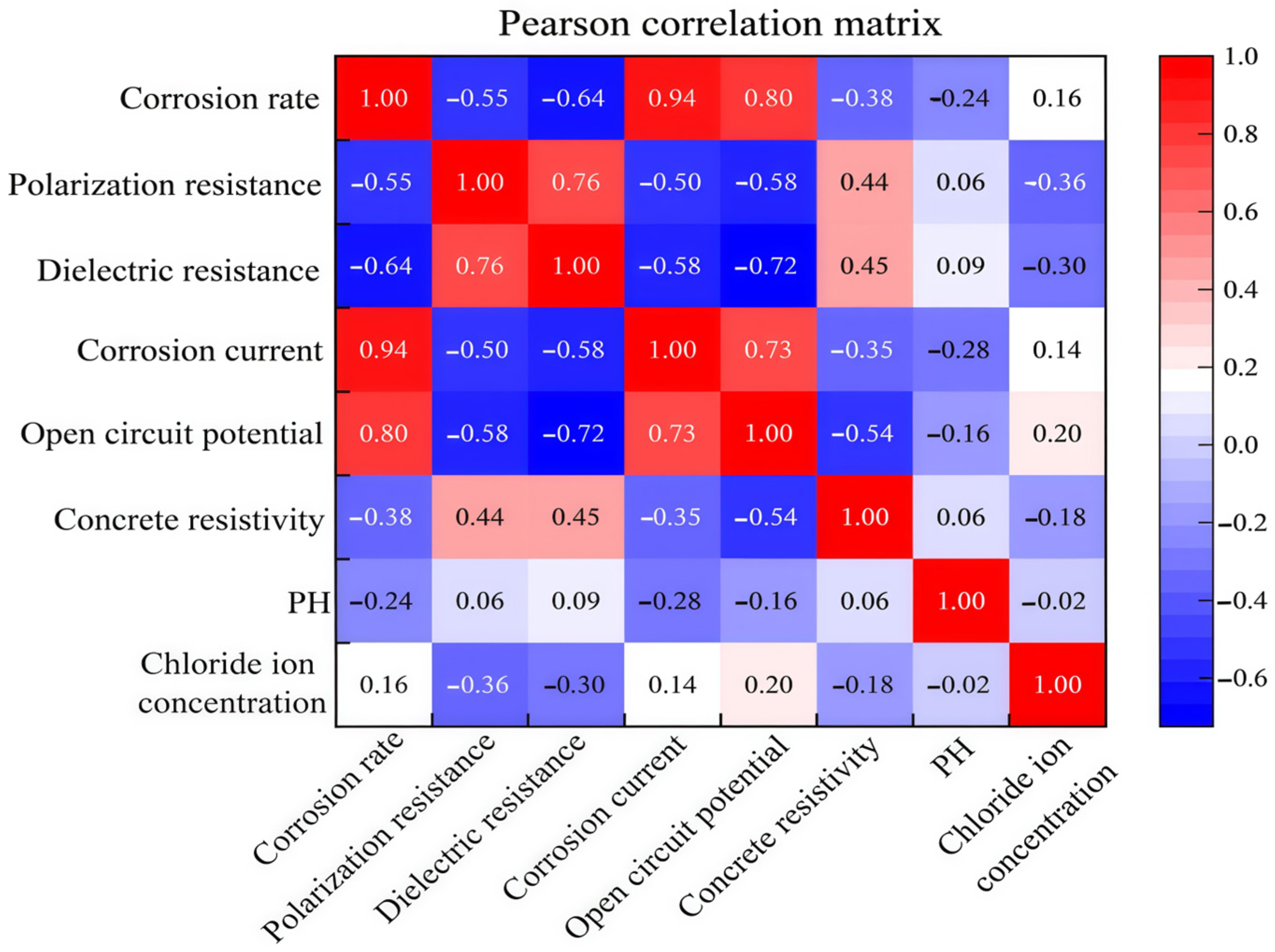
Multi-physical feature fusion: In this study, strong correlation auxiliary features such as corrosion current and concrete resistivity are integrated by carrying out correlation coefficient analysis, which significantly improves the model’s ability to characterize the coupling effects of complex environments compared with a single feature.

(3)

Progressive training strategy: A “chunked progressive” training strategy is proposed to expand the prediction horizons in phases, which effectively alleviates the error accumulation problem in multi-step prediction.

(4)

Verification of cross-engineering generalization capability: In view of the shortcomings of existing studies that rely on single-system data, cross-engineering tests on prestressed steel-cylinder concrete pipelines in coastal areas are added. Experiments show that the prediction framework proposed in this paper has good adaptability to similar projects.

2. Research Methods and Principles

2.1. Graph-Based Modeling of Multivariate Time Series

Compared with univariate forecasting, the core assumption of the multivariate time series forecasting task lies in the existence of complex interactive dependencies between variables, and the model forecasting not only focuses on the historical data evolution law of a single variable, but also emphasizes the analysis of the dynamic coupling effect between different variables. From the graph perspective, the variables can be abstracted as nodes in the graph structure, from which potential associations between time series can be mined according to the characteristics of graph neural network arrangement invariance, local connectivity, and combinability. However, there are two problems when applying graph neural networks to time series prediction scenarios: first, in most cases, multivariate time series data lack a displayed graph structure; second, predefined graph structures usually need to be optimized in parallel with model training.

MTGNN can be targeted to solve the above multivariate time series prediction problem by dynamically and adaptively learning the temporal dependencies between nodes while optimizing the joint modeling of graphs and time series. MTGNN is mainly composed of three parts: graph learning layer, temporal convolution module, and graph convolution module, and its specific network structure is shown in Figure 2. The 1 × 1 convolution kernel first compresses the channel dimensions and maps the input features to the latent space. Then, the temporal convolution module and graph convolution module are stacked alternately to capture temporal and spatial correlations, respectively. The graph learning layer adaptively learns the hidden adjacency matrix between nodes. Residual connections and skip connections are introduced into the model to mitigate the gradient vanishing problem. The output module generates predictions by projecting the fused features to the target dimension.

2.2. Graph Learning Layer & Graph Convolution Module

The core mechanism of the graph learning layer is the dynamic generation of adjacency matrices, which is designed to enhance the model’s ability to represent complex spatio-temporal features by effectively capturing potential patterns of association between variables through adaptive graph structure learning. A non-assignment graph can be represented by the adjacency matrix $A={(a_{ij})}_{N\times N}$. The calculation of the graph learning layer is represented as Equation (1).

$$\left\{\begin{array}{l}{M}_1=\tanh (\alpha E_1{\theta }_1)\\ \begin{array}{l}{M}_2=\tanh (\alpha E_2{\theta }_2)\hfill \\ A=\mathrm{ReLU}(\tanh (\alpha (M_1{M}_2^T-M_2{M}_1^T)))\hfill \\ \begin{array}{ll}for & i=1,2,\cdots ,N\\ & idx=argtopk(A[i,:])\\ & A[i,-idx]=0\end{array}\hfill \end{array}\end{array}\right.$$

(1)

where $E_1$ and $E_2$ are the initialized node embeddings; ${\theta }_1$ and ${\theta }_2$ are learnable model parameters; $\alpha$ is the saturation rate that controls the activation function; $argtopk$ denotes the number of nearest nodes of the selected node to be predicted.

The graph convolution module is used to integrate the information from nodes and neighboring nodes, and a two-branch mix-hop propagation layer is used to process the input and output information from each node. The mix-hop propagation layer is calculated as shown in Equation (2).

$$\left\{\begin{array}{l}{H}^{(k)}=\beta H_{in}+(1-\beta )\tilde{A}H\hfill \\ H_{out}={\displaystyle \sum _{i=0}^K{H}^{(k)}}{W}^{(k)}\hfill \end{array}\right.$$

(2)

where $\beta$ is a hyperparameter to keep the proportion of original node information; $k$ denotes the depth of the propagation layer; $H_{in}$ denotes the inputs of the current layer (outputs of the previous layer); $H_{out}$ denotes the outputs of the current layer; and $\tilde{A}={\tilde{D}}^{-1}(A+I)$ where $\tilde{D}$ is a diagonal matrix and ${\tilde{D}}_{ii}=1+{\displaystyle \sum _j{A}_{ij}}$; $W^{(k)}$ denotes the parameter matrix of the $k$th layer.

The structure of the graph convolution module is shown in Figure 3.

2.3. Temporal Convolution Module

The temporal convolution module adopts a two-branch dilated inception layer structure, where each dilated inception layer contains multiple sets of one-dimensional dilated convolution kernels with different expansion rates to capture multi-scale temporal dynamic features. The two dilated inception layers are then nonlinearly transformed by accessing the tanh( ) activation function and the sigmoid( ) activation function, respectively. The dilated inception layer performs multi-scale feature extraction on the temporal data using multiple sets of 1D convolution kernels with different receptive fields and then integrates the feature maps generated by each convolution kernel, which is calculated as in Equation (3).

$$\left\{\begin{array}{l}z\ast f_{1\times k}(t)={\displaystyle \sum _{s=0}^{k-1}{f}_{1\times k}}(s)z(t-d\times s)\hfill \\ z=concat(z\ast f_{1\times k_1},\cdots ,z\ast f_{1\times k_l})\hfill \end{array}\right.$$

(3)

where $z$ represents the input sequence; $f_{1\times k}$ represents the $1\times k$ convolution kernel; $\ast$ is the symbol of the temporal convolution operation; $z\ast f_{1\times k}$ is the output of the temporal convolution; $t$ corresponds to the position of the element in the sequence; $d$ is the dilation factor; $concat( )$ performs the tensor splicing function.

The structure of the temporal convolution module is shown in Figure 4.

2.4. Skip Connection Layer & Output Module

The skip connection layer is in the form of a $1\times L_i$ standard convolution, where $L_i$ represents the length of the input sequence of the $i$th skip connection layer, which normalizes the information transmitted to the output module to ensure uniform input sequence length. The output module consists of two 1 × 1 standardized convolution layers, which are used to convert the input channel dimension into the target output dimension.

3. Multi-Step Prediction Framework for Multivariate Corrosion Information Based on Adaptive MTGNN

3.1. Brief Description of the Corrosion Rate Prediction Problem

The spatial inhomogeneity of the internal environment of the pipeline and the corrosion propagation mechanism lead to the spatial dependence of the corrosion rate at different locations of the pipe wall. The MTGNN-based corrosion rate prediction model proposed in this paper utilizes the graph learning module of MTGNN to adaptively find the latent spatial correlation between the corrosion states of each node to improve the prediction accuracy while capturing the time-dimensional information.

Let $Z_t=\left[z_{1,t},z_{2,t},\cdots ,z_{N,t}\right]\in R^{N\times D}$ denote the historical feature values of the $N$ corrosion monitoring nodes in the pipeline at time $t$, where $z_{i,t}=\left[z_{i,t,1},z_{i,t,2},\cdots ,z_{i,t,D}\right]$ denotes the $D$ feature values of the $i$th corrosion monitoring node at time $t$. Considering the existence of multiple sources of heterogeneous information in the actual node, the corrosion rate indicator can be combined with other auxiliary features. The first column of $Z_t$ is used as the corrosion rate (primary feature), and the rest of the columns are used as auxiliary features. Therefore, the corrosion information dataset of $T$ time steps for $N$ monitoring nodes can be represented as $X=\left[Z_1,Z_2,\cdots ,Z_T\right]\in R^{T\times N\times D}$. In order to realize the embedding of corrosion information in the graph, the spatio-temporal information graph of corrosion rate, constructed by treating the corrosion sensor at each location as a corrosion rate monitoring node, is shown in Figure 5. The graph of the corrosion rate is represented as $G=(V,E)$, where $V$ is the set of corrosion rate nodes, and $E$ is the set of edges between corrosion rate nodes. Given historical observations of the multivariate variable $X=\left[Z_1,Z_2,\cdots ,Z_T\right]$, the goal of the model is to predict the sequence of future values $Y=\left[Z_{T+1},Z_{T+2},\cdots ,Z_{T+Q}\right]$.

In this paper, we set $T_{in}$ = 15,$T_{out}$ = 6, i.e., the historical data of the last 15 time nodes are used to predict the corrosion rate of the next 6 time nodes. In order to avoid the limitations of manually defining the graph structure and highlight the adaptability of the dynamic graph structure to the spatial heterogeneity of pipeline corrosion, this paper adopts the adaptive MTGNN as the core framework, and the specific steps of the pipeline corrosion spatio-temporal correlation model constructed in this paper are as follows:

(1)

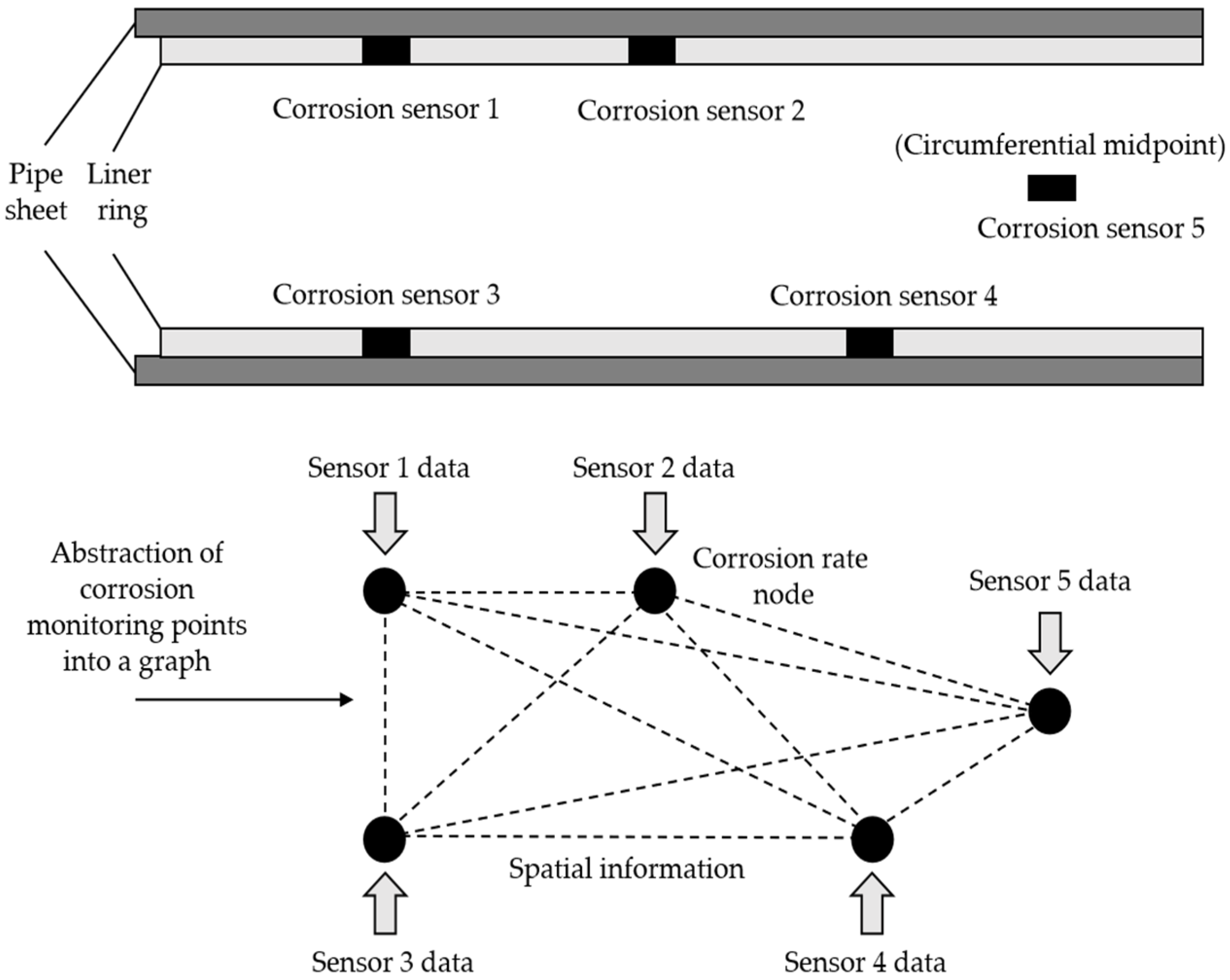
Generate initial node embedding vectors based on the physical location coordinates of the monitoring points and multi-feature data as input to the graph learning layer.

(2)

Calculate the similarity between nodes through a two-branch structure and use the graph learning layer to generate a dynamic adjacency matrix that captures the implicit spatial dependencies between nodes.

(3)

A top-k strategy is used to select the critical neighbors of each node, and non-critical connections are set to zero to optimize the matrix sparsity and reduce the computational complexity.

(4)

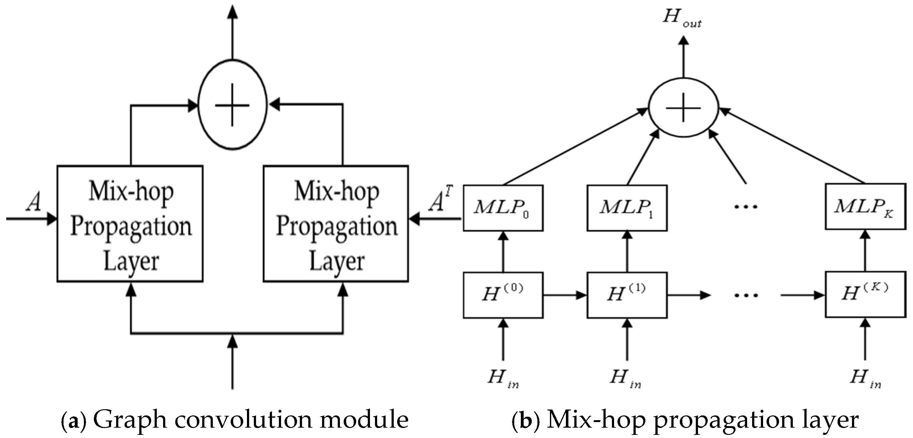
Input the dynamic adjacency matrix into the graph convolution module and integrate the multi-feature information of the node itself and its neighbors through the mix-hop propagation layer to generate the spatial feature representation.

(5)

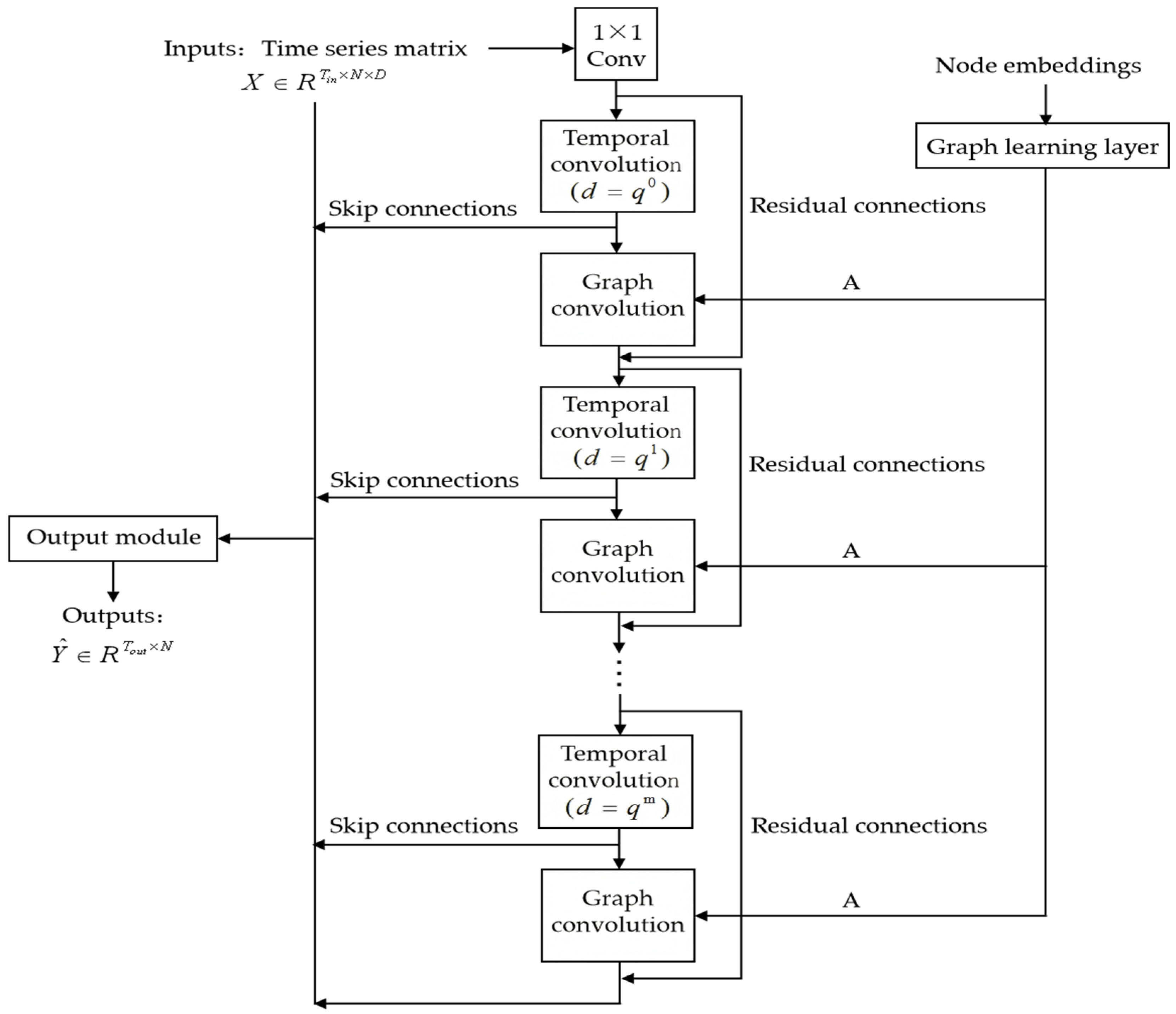
Alternately stack the graph convolution module and the temporal convolution module to extract spatial and temporal features, respectively, retain the original information through residual connections, skip connections to transfer features across layers, and finally output the predicted corrosion rate that integrates spatial and temporal information.

To address the problem of error accumulation in multi-step prediction, this paper proposes a “chunked progressive” training strategy based on the idea of “curriculum learning” [30]. The method gradually expands the prediction horizon of the model by decomposing the multi-step prediction task into multiple sub-blocks. At the beginning of training, the model only focuses on the prediction of local consecutive time steps, and as the training progresses, the neighboring sub-blocks are merged into a larger prediction block, which eventually covers the complete prediction range.

The specific implementation is as follows: the 6-step prediction is divided into 3 consecutive sub-blocks (1–2 steps, 3–4 steps, 5–6 steps), and the model is trained for a total of 100 epochs. The first 20 epochs of training focus on reducing the prediction error of step 1–2; the 21st to 40th epochs add the error calculation of step 3–4 on the basis of maintaining the prediction accuracy of step 1–2; the 41st to 60th epochs further introduce the error term of step 5–6; and the last 40 epochs uniformly optimize the full range of prediction errors of 1–6 steps. The design is based on incremental block expansion, which enables the model to gradually establish long-range dependence after local prediction is stabilized.

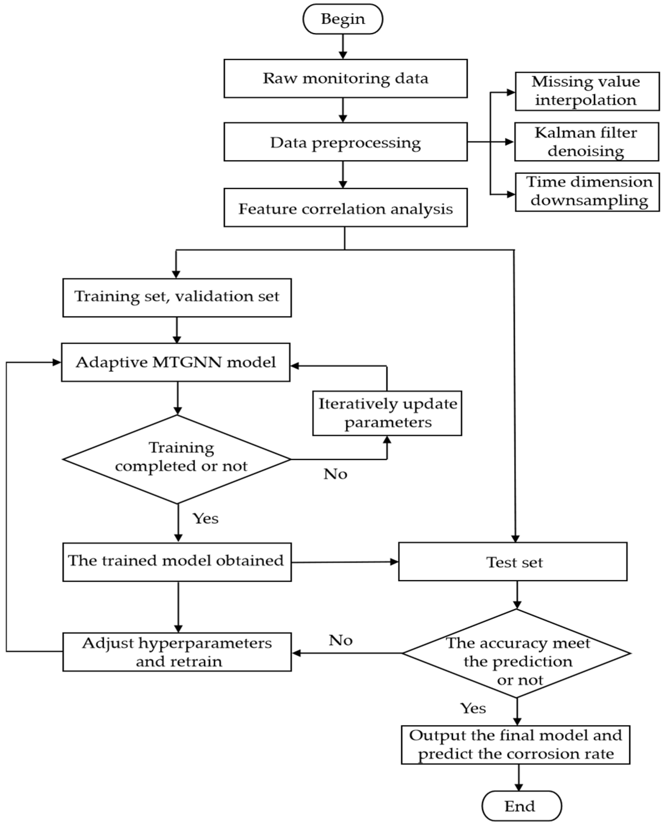
3.2. Prediction Process

The model prediction process is shown in Figure 6.

The corrosion rate prediction process based on the adaptive MTGNN model is as follows: firstly, the historical data of the corrosion monitoring locations are preprocessed; in order to explore the optimal performance of the model under multiple corrosion information, feature correlation analysis is carried out, and different combinations of feature variables are set up according to the correlation level; and then, the data are divided into training set, validation set, and test set. After that, the adaptive MTGNN model is used to train the training set for several epochs, and the hyperparameters are adjusted with the help of the validation set. Finally, the generalization performance of the model is evaluated with the test set, and if it does not meet the requirements, the hyperparameters are further optimized and retrained until the expected results are achieved. The optimal combination of input feature variables can be determined by comparing and analyzing the prediction results of different input features.

3.3. Evaluation Index

In order to evaluate the prediction performance of the model, the evaluation indices selected are the Mean Absolute Error (MAE), Root Mean Square Error (RMSE), and Mean Absolute Percentage Error (MAPE), with their calculation methods defined in Equations (4)–(6).

$$\mathrm{MAE}={\displaystyle \frac{1}{n}}{\displaystyle \sum _{i=1}^n\left|{\widehat{y}}_i-y_i\right|}$$

(4)

$$\mathrm{RMSE}=\sqrt{{\displaystyle \frac{1}{n}}{\displaystyle \sum _{i=1}^n{\left({\widehat{y}}_i-y_i\right)}^2}}$$

(5)

$$\mathrm{MAPE}={\displaystyle \frac{1}{n}}{\displaystyle \sum _{i=1}^n\left|\frac{{\widehat{y}}_i-y_i}{y_i}\right|}\times 100\%$$

(6)

where: $n$ is the number of samples; $y_i$ is the actual value of the $i$th sample; ${\widehat{y}}_i$ is the predicted value of the $i$th sample.

3.4. Comparison Models

In this paper, for corrosion rate prediction, two different forms of MTGNN are compared: adaptive MTGNN and non-adaptive MTGNN. The adaptive MTGNN dynamically generates adjacency matrices by computing node similarities using learnable graph structural parameters, whereas the non-adaptive MTGNN does not use the graph learning layer to capture spatial dependencies but only mines temporal features. In this paper, we set the adjacency matrix of non-adaptive MTGNN as a static unit matrix. In addition, in order to prove the effectiveness of the adaptive MTGNN model in the field of spatio-temporal forecasting, this paper also compares it with Long Short-Term Memory (LSTM) and Gated Recurrent Unit (GRU), which are two widely used forecasting models for time series.

4. Engineering Example

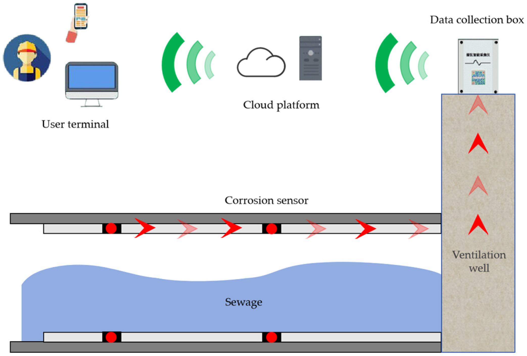
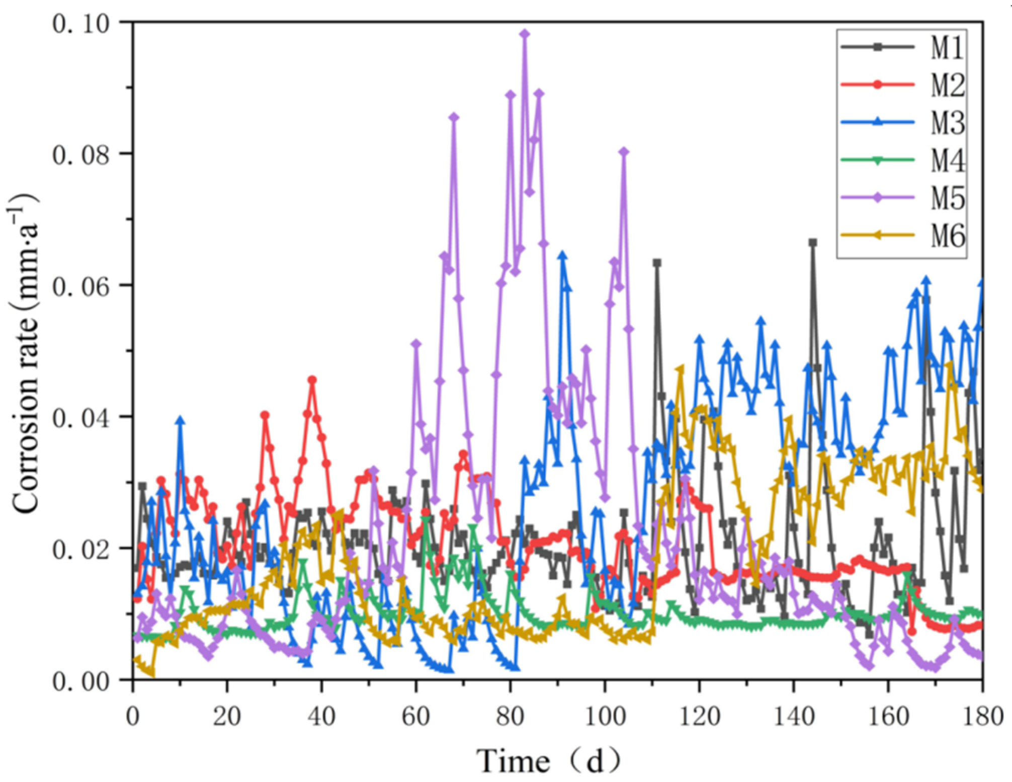
4.1. Overview of the Project

The data utilized in this research were obtained from an automated corrosion monitoring system implemented in a city’s concrete sewer pipelines. The data collection and transmission flowchart is shown in Figure 7. The monitoring equipment adopts a buried multi-probe corrosion sensor, which integrates the collector and multi-functional corrosion monitoring probe into one and can monitor multiple corrosion parameters in real time. The sensor cable is introduced into the special junction box reserved in the pipe section through the pre-embedded pipe and distributed along the longitudinal direction of the pipe section at multiple points. Due to the fluidity of the corrosive medium in the pipe, the closer monitoring points may collect the relevant results. This study selected a section with neighboring local monitoring points M1~M6 as an example of engineering data. The frequency of data collection is once every hour, and the collection period is from 21 July 2021 to 26 July 2024, with a total of 24,796 periods of data obtained.

4.2. Data Preprocessing and Model Settings

The experimental dataset covers 8 core indicators of pipeline corrosion: corrosion rate (CR), polarization resistance (PR), dielectric resistance (DR), corrosion current (CC), open circuit potential (OCP), concrete resistivity (RT), PH, chloride ion concentration (Cl-), which comprehensively reflect the corrosion state of the pipeline. By preprocessing the data, the data quality and the effectiveness of subsequent model training are ensured.

4.2.1. Missing Value Interpolation

Considering the instability of the sensor acquisition device, corrosion monitoring data often have missing values. First of all, the sample data should be processed for missing values. This paper uses linear interpolation along the time dimension to fill in the vacant values, and the relevant calculation method is shown in Equation (7).

$$x_t=x_i+\left({\displaystyle \frac{t-t_i}{t_j-t_i}}\right)·(x_j-x_i)$$

(7)

where $t_i$, $t_j$ is the start and end moments of the missing data interval; $x_i$ and $x_j$ denote the monitoring data values at moments $t_i$ and $t_j$, respectively; $x_t$ is the missing data compensation value of $t$ at any moment between $t_i$ and $t_j$ after interpolation.

4.2.2. Kalman Filter Denoising

In order to reduce the random noise interference of the sensor in the actual working conditions, after sorting according to the time order, the original data are processed for noise reduction using Kalman filtering, which minimizes the expected value of the estimation error and outputs the optimal estimation of the system state and is widely used for data noise reduction. The calculation method is shown in Equations (8) and (9).

$$X_{i+1}=(1-K_{i+1})X_i+K_{i+1}{Z}_{i+1}$$

(8)

$$K_{i+1}=(P_i+Q)/(P_i+Q+R)$$

(9)

where $X$ is the filtered output value, $Z$ is the input data, $K$ is the Kalman gain coefficient determined by the variance of the previous output value $P$, the system noise $Q$, and the measurement noise $R$.

4.2.3. Time Dimension Downsampling

Due to the low amplitude of daily fluctuations in the corrosion rate, for the convenience of prediction study, the method of calculating daily averages was used to downsample the sample data, changing the sampling frequency from 1 h to 1 day, and constructing a dataset using the average corrosion rate for each day, resulting in a total of 1000 sets of daily corrosion rate data, with the same processing applied to other corrosion indicators.

After the above preprocessing, the corrosion rate curves of the 6 corrosion monitoring points inside the pipeline in 6 months (to ensure visual clarity and to highlight the spatial differences between the monitoring points) are shown in Figure 8. As can be seen from Figure 8, the corrosion rates of different monitoring points have large differences, which reflects the influence of spatial location on the corrosion behavior. Therefore, consideration of the spatial characteristics of pipeline corrosion can help better mine the corrosion state information.

4.2.4. Feature Correlation Analysis

The key to achieving optimization of adaptive MTGNN under a multi-feature dataset is to determine the optimal input feature combination for the nodes. In the example, the degree of linear correlation between different features can be quantified by calculating the Pearson correlation matrix. The Pearson correlation coefficient ranges from −1 to 1, where a value of 1 indicates a perfect positive linear correlation between features, −1 indicates a perfect negative linear correlation, and 0 indicates that there is no linear correlation between features. The Pearson correlation coefficient is calculated in Equation (10).

$$r_{xy}={\displaystyle \frac{n(\sum xy)-(\sum x)(\sum y)}{\sqrt{([n\sum x^2-{(\sum x)}^2][n\sum y^2-{(\sum y)}^2])}}}$$

(10)

where $r_{xy}$ is the correlation coefficient between the two variables $x$ and $y$, $n$ is the number of observed samples, $\sum xy$ is the sum of the products of the two variables, and $\sum x$ and $\sum y$ are the respective sums of the variables $x$ and $y$.

From the calculation results in Figure 9, it can be seen that there is an obvious positive correlation between corrosion current (0.94), open circuit potential (0.80), and corrosion rate, i.e., an increase in corrosion current and open circuit potential usually causes an increase in corrosion rate. There is a strong negative correlation between polarization resistance (−0.55), dielectric resistance (−0.64), concrete resistivity (−0.38), and corrosion rate, which suggests that an increase in resistance-based detection indicators contributes to the reduction of corrosion rate. Other indicators, such as PH (−0.24) and chloride concentration (0.16), had a weak correlation with corrosion rate.

In this paper, three combinations of features are established as node inputs to the embedding layer based on the strength of the correlation between the remaining features and the Corrosion Rate (CR), which are grouped as shown in

Table 1. Three combinations of input features.

Number	Input Features	Instructions
1	CR	Single feature
2	CR, PR, DR, CC, OCP, RT	Strongly correlated features
3	CR, PR, DR, CC, OCP, RT, PH, Cl-	All features

. The optimal input features of the nodes can be obtained by comparing the prediction results of each combination, and then the optimal model can be further compared with other baseline models.

4.2.5. Division and Normalization of Dataset

All the data are divided into training set, validation set and test set according to 7:2:1. In order to optimize the model convergence, improve the training speed and prevent the gradient explosion, these 3 datasets are normalized with the mean and standard deviation of the training set, which is calculated as Equation (11).

$$\widehat{x}={\displaystyle \frac{x-mean(X_{\mathrm{train}})}{\mathrm{std}(X_{\mathrm{train}})}}$$

(11)

where $x$ is the original data; $\widehat{x}$ is the normalized data; $mean(X_{\mathrm{train}})$ denotes the mean of the training set $X_{\mathrm{train}}$; $\mathrm{std}(X_{\mathrm{train}})$ denotes the standard deviation of the training set $X_{\mathrm{train}}$.

4.2.6. Model Parameters Setting

The selection of model parameters is crucial to model performance. By referring to research experience in related fields, conducting multiple experiments for comparative analysis, and fully balancing the relationship between model complexity and computational resources, the following model parameter settings are ultimately obtained: the graph convolution module and the temporal convolution module are both set to 3, the graph convolution depth is 2, the dilated inception layer adopts a total of 4 convolution kernels: 1 × 2, 1 × 3, 1 × 4, and 1 × 7, and the potential spatial dimension is set to 40. The L₁ loss function (Mean Absolute Error) is selected as the optimization objective to minimize prediction deviations. The learning rate and weight decay value are both set to 0.001, and overfitting is prevented by using the dropout method, with the dropout rate configured as 0.2, the training batch size as 32, and the epochs as 100. Considering the large amount and the non-stationarity of actual monitoring data, Adam is chosen as the optimizer for the model.

4.3. Results and Analysis

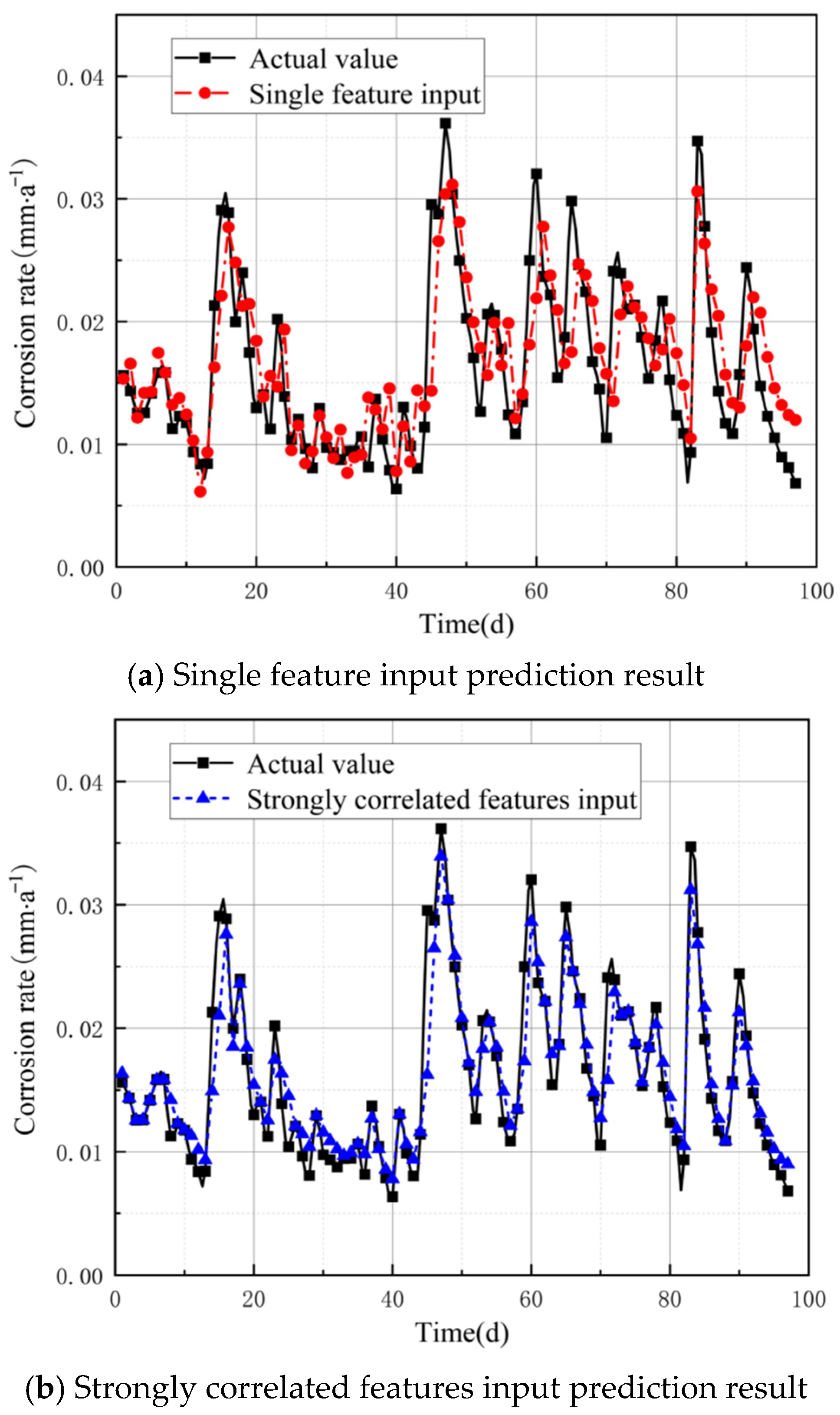
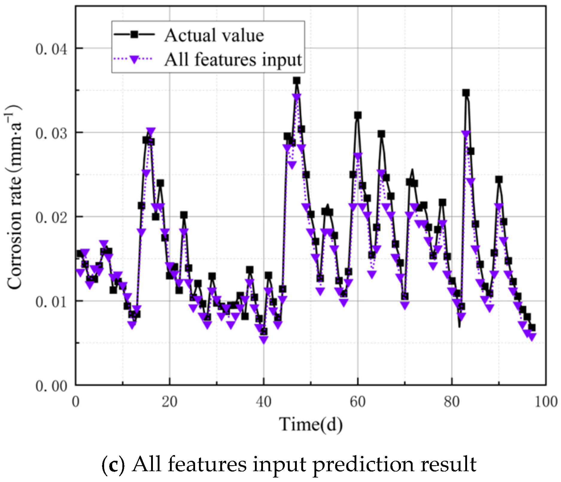
4.3.1. Prediction Results and Analysis Under Different Combinations of Input Features

In order to better illustrate the superiority of adaptive MTGNN in dealing with multi-feature non-smooth time series, this section first conducts a comparative experiment with three combinations of input features to determine the optimal input for the nodes. Taking the corrosion rate prediction results of monitoring point M1 as an example, the predictive performance of adaptive MTGNN under different input features is shown in Figure 10.

As shown in Figure 8, when the corrosion rate is relatively stable, the prediction results of the single feature input and the strongly correlated features input are not much different. When the corrosion rate fluctuates greatly, the strongly correlated features input performs better than the single feature input in capturing the peak of corrosion rate fluctuation, and it is more sensitive to the trend of data change. However, all features input will instead introduce redundant signals, making the information transfer between nodes less efficient and leading to a decrease in model prediction accuracy.

Table 2. Comparison of prediction results under different combinations of input features.

Input Features	MAE (×10−3)	RMSE (×10−3)	MAPE (%)
CR	1.948	2.512	14.225
CR, PR, DR, CC, OCP, RT	1.507	2.051	9.690
CR, PR, DR, CC, OCP, RT, PH, Cl-	1.801	2.169	11.216

further quantitatively analyzes the performance of the model under different combinations of input features. From Table 2, it can be seen that the MAE of the data is reduced by 22.64% and 16.32%, the RMSE is reduced by 18.35% and 5.44%, and the MAPE achieves the minimum value when the prediction is made by using the strongly correlated features, as compared with the single feature input and the all features input, respectively. The experimental results show that the predictions of the model are closest to the actual values when the node inputs are strongly correlated features.

The prediction framework proposed in this paper first screens out strongly correlated features as graph node inputs and then integrates the dynamic patterns among covariates through the graph convolution module and the temporal convolution module, which can extract complementary information for reflecting the volatility of the target variable and overcome the limitations of single-feature modeling.

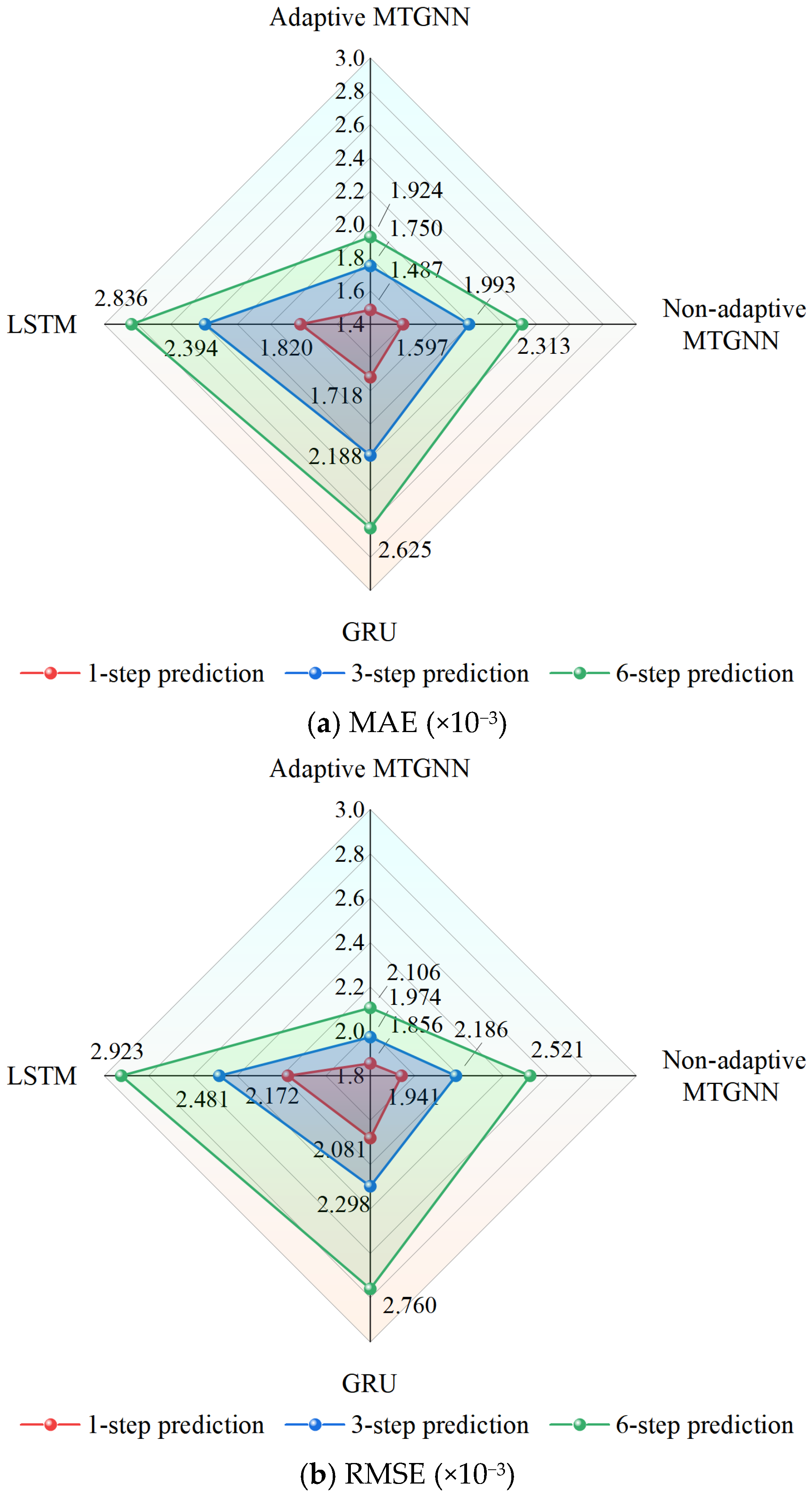
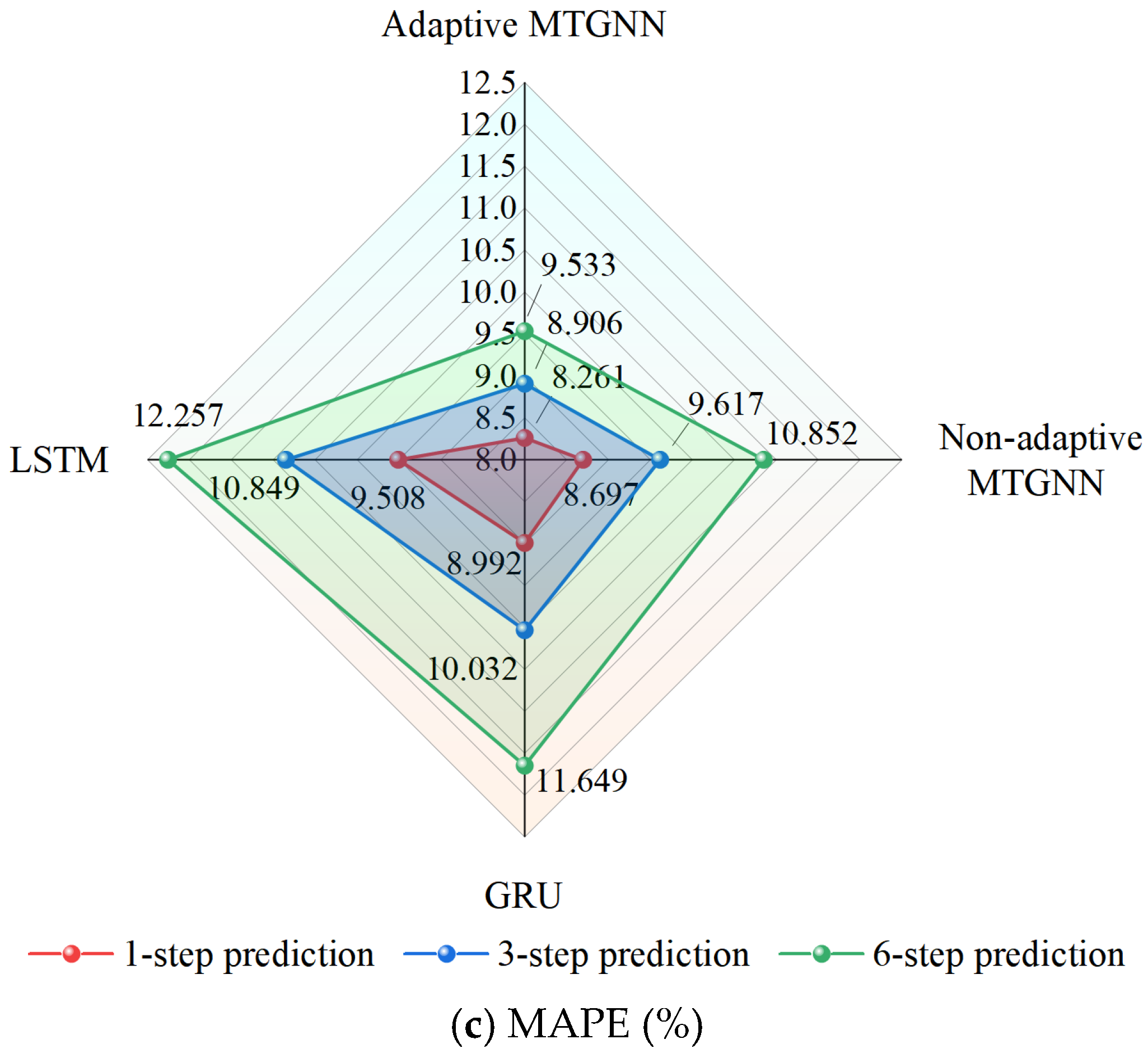
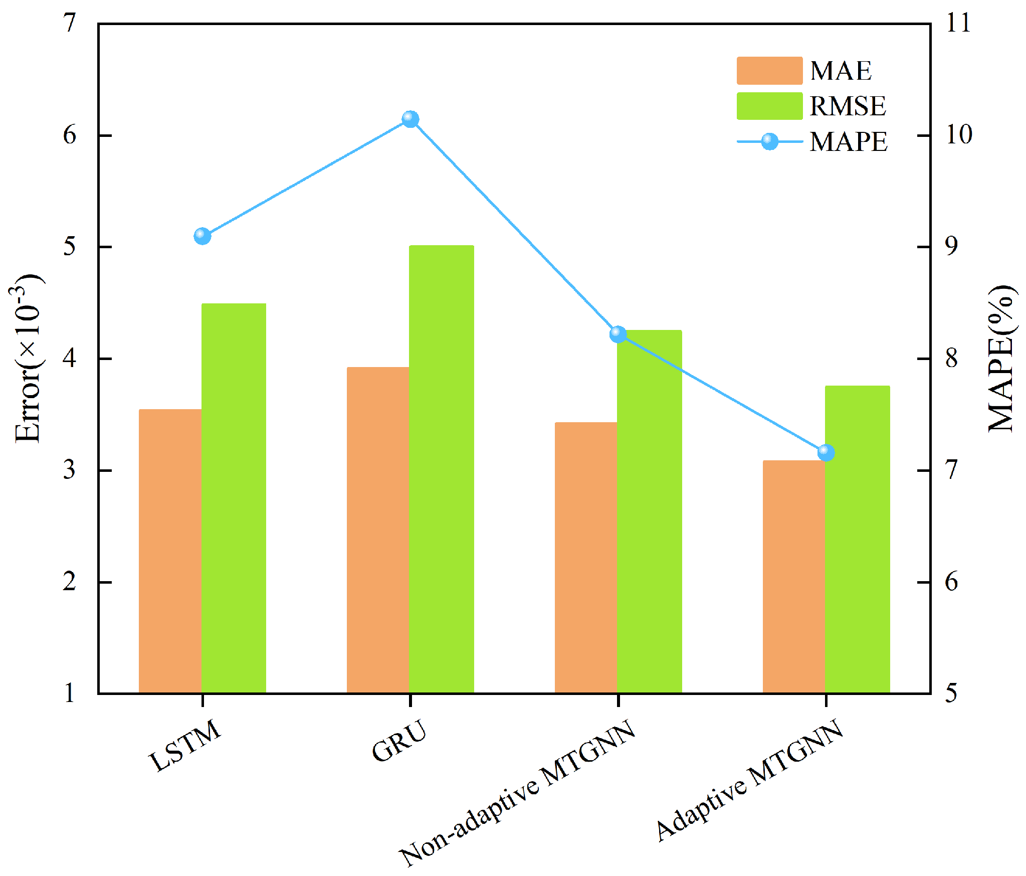
4.3.2. Comparative Analysis of the Performance of Different Prediction Models

This section compares the performance difference between adaptive MTGNN and other baseline models under different prediction steps based on determining the optimal input features. Since all models are for multi-node predictions, the value of the evaluation index is the average of the prediction errors of all nodes. The comparison of prediction accuracy of the four models under the three evaluation indices is shown in

Table 3. Comparison of predictions of different models at different prediction steps.

Evaluation Index	Prediction Model	Prediction Step Size
		1	3	6
MAE (×10−3)	Adaptive MTGNN	1.487	1.750	1.924
	Non-adaptive MTGNN	1.597	1.993	2.313
	GRU	1.718	2.188	2.625
	LSTM	1.820	2.394	2.836
RMSE (×10−3)	Adaptive MTGNN	1.856	1.974	2.106
	Non-adaptive MTGNN	1.941	2.186	2.521
	GRU	2.081	2.298	2.760
	LSTM	2.172	2.481	2.923
MAPE (%)	Adaptive MTGNN	8.261	8.906	9.533
	Non-adaptive MTGNN	8.697	9.617	10.852
	GRU	8.992	10.032	11.649
	LSTM	9.508	10.849	12.257

, and the comparison results of the error improvement percentage of the adaptive MTGNN compared to other models under three evaluation indices are shown in

Table 4. Comparison of the percentage of error improvement (%) under different evaluation indices.

Evaluation Index	Prediction Model	Prediction Step Size
		1	3	6
MAE (×10−3)	Non-adaptive MTGNN	6.59	12.12	16.82
	GRU	13.44	20.01	26.70
	LSTM	18.30	26.90	32.16
RMSE (×10−3)	Non-adaptive MTGNN	4.38	9.70	16.46
	GRU	10.81	14.10	23.70
	LSTM	14.55	20.44	27.95
MAPE (%)	Non-adaptive MTGNN	5.01	7.39	12.15
	GRU	8.13	11.22	18.01
	LSTM	13.12	17.90	22.22

.

The results show that for 1-step prediction, the MAE of adaptive MTGNN decreases by 6.59%, 13.44%, and 18.30% compared with non-adaptive MTGNN, GRU, and LSTM, respectively. For 3-step prediction, the MAE decreases by 12.12%, 20.01%, and 26.90%, respectively. For 6-step prediction, the MAE decreases by 16.82%, 26.70%, and 32.16%, respectively. In addition, the improvement in RMSE error ranges from 4.38% to 27.95%, and in the MAPE error, it ranges from 5.01% to 22.22% over the prediction range of steps 1–6. It can be seen that the adaptive MTGNN significantly outperforms the other models on all three evaluation indices.

The primary reason that adaptive MTGNN significantly improves corrosion rate prediction results is that the nature of the corrosion data is better suited to the MTGNN modeling assumptions regarding temporal and spatial dependence. When the concrete in an area is subjected to severe corrosion, this corrosion state may gradually affect the surrounding areas with the flow of sewage and the diffusion of corrosive substances. MTGNN leverages graph-based information propagation to effectively integrate information from different nodes, fully extracting spatial features to enhance prediction accuracy for each node. GRU and LSTM lack a specialized structural design for dealing with spatial and temporal series data, and it is difficult for these methods to effectively model multivariate time series data when spatial information is implied between prediction targets.

Figure 11 shows the difference in prediction accuracy between the adaptive MTGNN and other models more intuitively in the form of radar charts. In the radar charts, the region corresponding to the adaptive MTGNN under each evaluation index is closer to the center of the radar chart. As the prediction step size increases, the error increment is the smallest, and the error improvement of each index is also gradually improved, indicating that the “chunked progressive” training strategy adopted in this paper has an outstanding advantage in multi-step prediction.

In Table 3 and Table 4, the prediction results of the adaptive MTGNN are consistently better than those of the non-adaptive MTGNN, which reveals the significant advantage of the adaptive adjacency matrix in learning the spatial features of the corrosion rate. When the adjacency matrix in MTGNN is a static unit matrix, the node information can only be propagated within each node itself, and there is no effective information aggregation with other nodes, so it is difficult for the model to learn the changing patterns of corrosion information in space. Adaptive MTGNN overcomes the shortcomings of artificially defining the graph structure and can dynamically adjust the connection weights between nodes according to the inputs, thus improving the prediction accuracy of the region as a whole.

4.4. Generalization Performance Verification

In order to further investigate the performance of the method proposed in this paper on other similar projects, a prestressed steel-cylinder concrete pipe with the same monitoring system in a coastal area is tested, which has similar service environment and material properties as the original experimental subject, and multiple corrosion sensors are deployed in key sections. The model structure and modeling process are preserved unchanged during the testing process, and strong correlation features are selected as inputs to verify the generalization ability of the framework. Meanwhile, for comparative analysis, the same hyperparameters are used to construct LSTM, GRU, and non-adaptive MTGNN models separately. The performance comparison of similar engineering models is shown in

Table 5. Comparison of similar engineering model performances.

Prediction Model	MAE (×10−3)	RMSE (×10−3)	MAPE (%)
LSTM	3.538	4.484	9.093
GRU	3.916	5.003	10.144
Non-adaptive MTGNN	3.419	4.245	8.216
Adaptive MTGNN	3.081	3.780	7.157

. In order to visually compare the differences, the data of each index of the above models are plotted and displayed as bar charts and line graphs, and the comparison results are shown in Figure 12. From Figure 12, it can be seen that the adaptive MTGNN model also shows good performance in similar engineering, and its MAE, RMSE, and MAPE are better than the other models, which confirms the effectiveness of the spatio-temporal correlation feature extraction mechanism in cross-engineering scenarios.

The prediction framework proposed in this paper is based on multivariate feature fusion and dynamic graph structure learning, which improves the robustness of the model to noise and distributional bias and can be generalized to similar engineering applications. Follow-up studies can further explore how to optimize the model structure and parameters to further improve its adaptability under different engineering conditions.

5. Conclusions

In this paper, a corrosion rate prediction framework based on adaptive MTGNN multi-feature spatio-temporal correlation analysis is proposed for the corrosion rate prediction of pipeline walls, and the actual monitoring data of drainage pipeline in a city is used as an example to explore the prediction performance of the model under multivariate input and different prediction steps. The following conclusions are obtained:

(1)

By introducing strongly correlated features in the node embedding of the input layer, the prediction performance of the model is substantially improved compared with the single feature input and all feature input. Adaptive MTGNN captures the synergistic temporal patterns among multiple features in an end-to-end manner and is able to more accurately reflect the changing trends of time series. This result demonstrates the superior ability of adaptive MTGNN in modeling complex cross-variate information and effectively utilizing auxiliary features.

(2)

The deep learning model based on adaptive MTGNN to construct spatio-temporal graphs can extract the neighborhood aggregated spatio-temporal information and adaptively learn the internal graph structure through graph convolution and temporal convolution without the need for prior knowledge of edges. The experimental results show that the model increases the extraction of spatial features compared with the traditional time series prediction methods, which can achieve higher prediction accuracy and provide a reference for similar pipeline internal corrosion prediction problems.

(3)

In this study, a “chunked progressive” training strategy is used to decompose the multi-step prediction task into progressive sub-intervals, which enables the model to perform well in short-term prediction. However, there is still room for improvement in long-term prediction accuracy. Future research can introduce attention mechanisms or Transformer architectures to dynamically allocate importance to different time steps, alleviating error accumulation.

(4)

The fixed-size dilated convolution kernels used in this paper may lack flexibility when dealing with a large amount of non-stationary corrosion fluctuation data, making it difficult to adaptively adjust to match heterogeneous temporal features in complex environments. Future work will explore dynamic adjustable convolution kernel mechanisms, optimizing kernel size selection by integrating data-driven and physical prior knowledge, while combining lightweight strategies to reduce computational costs, thereby enhancing the model’s generalization ability to nonlinear spatio-temporal dynamics and engineering applicability.

References

1. Wu, E.B.; Wang, N.C.; Wang, K.L.; Zhang, J. Reasons and countermeasures for corrosion and leakage of sewage pipelines in public works. Total Corros. Control 2023, 37, 96–100+112. [Google Scholar] [CrossRef]
2. Zhao, L.; Qi, G.; Dai, Y.; Ou, H.X.; Xing, Z.X.; Zhao, L.; Yan, Y.F. Integrated dynamic risk assessment of buried gas pipeline leakages in urban areas. J. Loss Prev. Process Ind. 2023, 83, 105049. [Google Scholar] [CrossRef]
3. Wang, Y.J.; Su, F.; Guo, Y.; Yang, H.L.; Ye, Z.J.; Wang, L.B. Predicting the microbiologically induced concrete corrosion in sewer based on XGBoost algorithm. Case Stud. Constr. Mater. 2022, 17, e01649. [Google Scholar] [CrossRef]
4. Wang, Y.C.; Xu, L.Y.; Sun, J.L.; Cheng, Y.F. Mechano-electrochemical interaction for pipeline corrosion: A review. J. Pipeline Sci. Eng. 2021, 1, 1–16. [Google Scholar] [CrossRef]
5. Mahdi, S.; Mojtaba, M.; Xue, Y.D.; Zhang, Y.; Wu, C.L. Time-Variant System Reliability Analysis of Concrete Sewer Pipes under Corrosion Considering Multiple Failure Modes. ASCE-ASME J. Risk Uncertain. Eng. Syst. Part A Civ. Eng. 2023, 9, 04023002. [Google Scholar] [CrossRef]
6. Zhu, Y.S.; Cai, K.; Hu, B.W.; Xia, Y.Q.; Hu, T.Y.; Huang, Y. Research Progress on Characteristics and Prediction Modelsof Carbon Dioxide Induced Corrosion forSubmarine Pipelines. J. Chin. Soc. Corros. Prot. 2023, 43, 1225–1236. [Google Scholar] [CrossRef]
7. Gao, X.L.; Wang, L.N.; Liu, W. Study on Internal Corrosion of Concrete Sewer Pipelines. Struct. Eng. 2020, 36, 71–79. [Google Scholar] [CrossRef]
8. Wu, Z.; Wang, Q.; Hu, J.X.; Tang, Y.; Zhang, Y.N. Integrating model-driven and data-driven methods for fast state estimation. Int. J. Electr. Power Energy Syst. 2022, 139, 107982. [Google Scholar] [CrossRef]
9. Li, B.H.; Wang, H.Y.; Li, J.; Lu, G.Q. Integrating model-driven and data-driven methods for under-frequency load shedding control. Electr. Power Syst. Res. 2025, 238, 111103. [Google Scholar] [CrossRef]
10. Wang, D.; Zou, Y.F.; Geng, H.J. Prediction of Corrosion Rate of Oil and Gas Pipelines Based on Grey System Theory. Total Corros. Control 2024, 38, 162–167. [Google Scholar] [CrossRef]
11. Luo, Z.S.; Yao, M.Y.; Luo, J.H.; Wang, X.W. Prediction Model of External Corrosion Rate of Submarine Pipeline Based on PCA-BAS-PPR. Mater. Prot. 2019, 52, 64–69+74. [Google Scholar] [CrossRef]
12. Bilal, M.; Idris, O.; Serdar, D.; Syuhaida, I.; Hussaini, W. Influence of Artificial Intelligence in Civil Engineering toward Sustainable Development—A Systematic Literature Review. Appl. Syst. Innov. 2021, 4, 52. [Google Scholar] [CrossRef]
13. Aref, A.; Gholamreza, N.; Shahin, G.; Hossein, H. Machine-Learning Applications in Structural Response Prediction: A Review. Pract. Period. Struct. Des. Constr. 2024, 29, 03124002. [Google Scholar] [CrossRef]
14. Vagelis, P. A Glimpse into the Future of Civil Engineering Education: The New Era of Artificial Intelligence, Machine Learning, and Large Language Models. J. Civ. Eng. Educ. 2025, 151, 02525001. [Google Scholar] [CrossRef]
15. Sun, Z.; Li, Y.L.; Li, Y.Q.; Su, L.; He, W.D. Investigation on compressive strength of coral aggregate concrete: Hybrid machine learning models and experimental validation. J. Build. Eng. 2024, 82, 108220. [Google Scholar] [CrossRef]
16. Hu, J.; Xia, C.J.; Wu, J.H.; Dong, F.H. Estimating the pile-bearing capacity utilizing a reliable machine-learning approach. Multisc. Multidiscip. Model. Exp. Des. 2025, 8, 217. [Google Scholar] [CrossRef]
17. Qu, Z.H.; Tang, D.Z.; Hu, L.H.; Chen, H.J.; Li, H.X.; Jia, H.Y.; Wang, Z.; Zhang, L. Prediction of H2S Corrosion Products and Corrosion Rate Based on Optimized Random Forest. Surf. Technol. 2020, 49, 42–49. [Google Scholar] [CrossRef]
18. Li, X.H.; Jia, R.C.; Zhang, R.R.; Yang, S.Y.; Chen, G.M. A KPCA-BRANN based data-driven approach to model corrosion degradation of subsea oil pipelines. Reliab. Eng. Syst. Saf. 2022, 219, 108231. [Google Scholar] [CrossRef]
19. Luo, Z.S.; Du, D.; Luo, J.H.; Wang, X.W. Research on the effectiveness of a combined model for predicting the corrosion rate of pipelines—CNN and LSTM models based on attention mechanism enhancement. J. Saf. Environ. 2024, 24, 4263–4269. [Google Scholar] [CrossRef]
20. Canonaco, G.; Roveri, M.; Alippi, C.; Podenzani, F.; Bennardo, A.; Conti, M.; Mancini, N. A transfer-learning approach for corrosion prediction in pipeline infrastructures. Appl. Intell. 2021, 52, 7622–7637. [Google Scholar] [CrossRef]
21. Wang, G.Q.; Wang, C.Q.; Shi, L.H. Corrosion Rate Prediction for Submarine Multiphase Flow Pipelines Based on Multi-Layer Perceptron. Atmosphere 2022, 13, 1833. [Google Scholar] [CrossRef]
22. Saputra, A.N.; Riza, S.L.; Setiawan, A.; Hamidah, I. A Systematic Review for Classification and Selection of Deep Learning Methods. Decis. Anal. J. 2024, 12, 100489. [Google Scholar] [CrossRef]
23. Wang, H.; Wang, B.L.; Cui, C.X. Deep Learning Methods for Vibration-Based Structural Health Monitoring: A Review. Iran. J. Sci. Technol. Trans. Civ. Eng. 2023, 48, 1837–1859. [Google Scholar] [CrossRef]
24. Chen, Z.; Yu, J.M.; Bindiganavile, V.; Yi, C.F.; Shi, C.J.; Hu, X. Time and spatially dependent transient competitive antagonism during the 2-D diffusion-reaction of combined chloride-sulphate attack upon concrete. Cem. Concr. Res. 2022, 154, 106724. [Google Scholar] [CrossRef]
25. Baji, H. Stochastic modelling of concrete cover cracking considering spatio-temporal variation of corrosion. Cem. Concr. Res. 2020, 133, 106081. [Google Scholar] [CrossRef]
26. Li, Z.; Ding, S.W.; Liu, X.; Yang, X.H.; Wei, L.X. Numerical Analysis of Structural Performance Degradation of Sewage Shield Tunnel Segment. Tunnel Constr. 2016, 36, 1207–1215. [Google Scholar]
27. Liu, B.S.; Tong, Y.; Gao, Y.X.; Liu, H.B.; Wu, M.N.; Bai, Y. Research Progress on Microbial Corrosion of Concrete in Sewage Pipelines. Corros. Prot. 2022, 43, 7–13. [Google Scholar]
28. Wang, Z.W. Analysis on Corrosion Rule and Mechanical Properties of Underground Circular Concrete Drainage Pipe. Master’s Thesis, Chongqing University, Chongqing, China, 2012. [Google Scholar]
29. Wu, Z.H.; Pan, S.R.; Long, G.D.; Jiang, J.; Chang, X.J.; Zhang, C.Q. Connecting the Dots: Multivariate Time Series Forecasting with Graph Neural Networks. In Proceedings of the 26th ACM SIGKDD International Conference on Knowledge Discovery & Data Mining, Virtual, 23–27 August 2020; pp. 753–763. [Google Scholar] [CrossRef]
30. Bengio, Y.; Louradour, J.; Collobert, R.; Weston, J. Curriculum Learning. In Proceedings of the 26th Annual International Conference on Machine Learning (ICML), Montreal, QC, Canada, 14–18 June 2009; pp. 41–48. [Google Scholar] [CrossRef]
Figure 1. Examples of pipeline corrosion failure.
Applsci 15 05686 g001
Figure 2. Network structure of MTGNN.
Applsci 15 05686 g002
Figure 3. Structure of graph convolution module.
Applsci 15 05686 g003
Figure 4. Structure of temporal convolution module.
Applsci 15 05686 g004
Figure 5. Spatio-temporal information map of corrosion rate.
Applsci 15 05686 g005
Figure 6. Flow of corrosion rate prediction based on adaptive MTGNN model.
Applsci 15 05686 g006
Figure 7. Data collection and transmission process.
Applsci 15 05686 g007
Figure 8. Corrosion rate curves of different monitoring points.
Applsci 15 05686 g008
Figure 9. Pearson correlation matrix of pipeline corrosion data.
Applsci 15 05686 g009
Figure 10. Comparison of prediction results under different combinations of input features.
Applsci 15 05686 g010aApplsci 15 05686 g010b
Figure 11. Representation of the prediction accuracy of different models by radar charts.
Applsci 15 05686 g011aApplsci 15 05686 g011b
Figure 12. Comparison of various metrics for different models.
Applsci 15 05686 g012