Abstract
Modern electric machines are attracting the greatest interest from the research community due to their current increasing number of applications, including electric vehicles and wind power generators. Their use requires the development of complex regulators, where predictive controllers appear as interesting and viable alternatives in recent research works. Although these controllers have an easy formulation and high flexibility to incorporate different control objectives in multidimensional systems, they have limitations that require attention and limit their application: a high computational cost and current harmonic content. This work presents a novel controller that focuses on these limitations, where the additional degree of freedom introduced in the predictive controller through the lead-pursuit guidance law concept is combined with the use of virtual voltage vectors to reduce the harmonic content in a controlled drive. The effectiveness of the proposed controller is explored using a five-phase drive and several figures of merit, such as the root mean square error in current tracking, the total harmonic distortion in the stator currents, and the number of switching commutations per cycle. Different predictive controllers are compared with the proposal in terms of speed regulation, stator current control, and steady-state performance, where the results obtained are analyzed to show the interest, improvements, and limitations of the proposal.
1. Introduction
The control of electric machines using electronic converters has an important role in modern societies and is the basis for many industrial applications such as electric vehicles, elevators, wind generators, and robots [1,2]. They require accurate dynamic regulations that can be achieved by the adequate control of the static current. Traditional control methods that use continuous control variables must use specific modulation phases, such as pulse width modulation (PWM) or its variations [3]. For multiphase drives, the extension of such techniques poses problems due to the existence of multiple planes in static current space: α-β, x1-y1, etc. For example, in distributed multiphase winding machines, the only current producing torque is the α-β component, while others only contribute to losses [4]. In this case, model predictive control (MPC) has recently appeared as an interesting and beneficial control method compared to traditional controllers [5]. In the 1960s, the concept of MPC was developed, and for a long time, its main application fields were limited to systems with slow dynamic responses, such as the petrochemical industry, which allows the performance of the required calculations and the high computational cost of the controller [6]. This use was recently extended to modern electric devices, such as multiphase drives [7], where the reasons for this interest are the greater complexity and number of variables in the multiphase drive and the intuitive and flexible formulation of the MPC technique. MPC can now be considered a promising control methodology in multiphase drives, where it presents an easy formulation and high flexibility for incorporating different control objectives [8].
However, the application of MPC in multiphase drives faces some limitations that require attention [9,10,11]. One limitation is the implementation of the controller. MPC is intensive in computation, and a limit on the sampling frequency is found for any given computing hardware [12]. Many attempts have been reported to decrease this computational load, with most of them based on a reduction in available control vectors [13], the definition of search techniques based on the physical considerations of the system to avoid the usual exhaustive search for finding the control action [14], or the simplification of the combinatorial search [15]. For example, the computational cost of a five-phase drive is reduced using a subset of voltage vectors available in the prediction algorithm in [16] or by eliminating the need for iteration in [17]. But the dependence of MPC on ‘uncertainties’ in the real system that affect the predictive model (i.e., non-measurable system variables or the discrepancy between actual and estimated or measured values of electrical parameters during normal drive operation) is particularly critical in these lower complexity MPC schemes [18], and the incorporation of more robust controllers, such as deadbeat strategies, is mandatory to achieve satisfactory drive performance [18,19].
A second important limitation is caused by the absence of an explicit modulation stage due to the fixed-time discretization nature of MPC, which produces not only high-harmonic components but also interharmonics and electrical noise in the drive, particularly for low values of the stator impedance [20]. While harmonics refer to current and voltage waveforms with frequencies that are multiples of the fundamental power frequency and appear due to the power converters used in variable-frequency drives, an important portion of waveform distortion is due to the interharmonics (not integer harmonics) that include subharmonics below the fundamental frequency when predictive controllers are utilized. All harmonic components can cause various problems in the electrical drive, including overheating the equipment, erratic behavior, and reduced efficiency. However, subharmonic currents and the heat generated by their losses can damage the electrical machine faster than other causes, such as voltage imbalance [21,22]. Again, attempts have been made to solve this issue, and recent research works mitigate the situation by applying two or more switching vectors during the same sampling period. For example, zero and active voltage vector combinations are applied at each sampling time in [23]. The active voltage vector is selected in response to conventional MPC optimization problems, and the time of application is calculated online using a linear and reduced-order model that depends on the predicted, measured, and reference values of the controlled variable. Similar approaches can be found in [24], using appropriate PWM methods to ensure fixed switching frequencies. An alternative strategy is to use offline computation and definition of available voltage vectors. These voltage vectors are called virtual voltage vectors (VVVs), which are basically predefined voltage models that ensure low average voltages in the xi-yi plane [25]. The obtained results have demonstrated an improvement in controller efficiency by reducing the harmonic content in the xi-yi planes at the cost of higher switching frequencies and lower available voltage limits [26].
In this context, a predictive control action is defined in [27] where variable control times are utilized. The proposal is particularly relevant because it adds an extra degree of freedom to the control action with nonuniform control frequencies, which allows higher temporal resolutions and mitigates the computational cost of the predictive controller. The motivation of our work is to extend the idea in [27], introducing VVV to reduce the harmonic content of the controlled system and simplify the control algorithm, where the x-y plane is no longer considered. The rest of the paper is organized as follows. The next section details the system under study, which is based on a five-phase induction motor (5pIM) drive. Then, the proposed controller, which combines the lead-pursuit and VVV concepts, is shown in Section 3. The proposed analysis and the results obtained are presented in Section 4, while the conclusions are finally indicated in Section 5.
2. The Case Study: Five-Phase Distributed Winding Induction Motor Drive Using a Conventional Two-Level VSI
The analyzed system is based on a 5pIM, a five-phase two-level voltage source inverter (5p2L-VSI) constructed from two SEMIKRON SKS 22F modules, and a DC power supply that acts as a DC link (KDC 300-50 from California Instruments Corporation, San Diego, CA, USA). The core of the control unit is an MSK28335 board with a TMS320F28335 digital signal processor model from Texas Instruments (Dallas, TX, USA). The feedback of the mechanical speed signal is provided by the GHM510296R/2500 encoder, while four LH25-NP Hall effect sensors from LEM are used to measure the stator phase-current signals. Note that the 5pIM has an isolated neutral point, a balanced load is assumed (vsa + vsb + vsc + vsd + vse = 0 and isa + isb + isc + isd + ise = 0), and a reduced number of current sensors (four instead of five) is used to obtain the stator phase currents. A DC motor is also used to generate load torque. The system is shown in Figure 1 and Figure 2, where some pictures of the hardware and the schematic diagram of the 5pIM drive are provided.
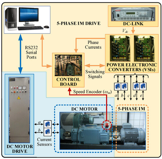
Figure 1.
Illustration diagram of the system used in the case study.
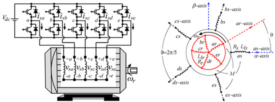
Figure 2.
Electrical scheme of the 5pIM drive.
The 5pIM was designed using equally distributed windings, ϑ = 2π/5, and the 5p2L-VSI generates 32 voltage vectors (30 active and 2 zero-voltage vectors), which is characterized by the switching vector [Sa Sb Sc Sd Se] as follows:
where the midpoint of the external power supply (Vdc) is considered the ground of the electrical system.
The electromagnetic performance of the machine can be represented with a set of phase-voltage equilibrium equations of the stator and the rotor in the stationary reference frame (a, b, c, d, e), obtained by assuming sinusoidal magnetomotive force distributions and uniform air gaps and neglecting core and magnetic losses:
where v and i denote the voltage and current, respectively, and the indices s and r represent the stator and rotor variables. Subscripts a, b, c, d, and e identify the phases considered, superscript T designates the transpose operator, and ωr is the electrical speed of the rotor. [I5] is the identity matrix of order 5; Rs and Rr are the resistances of the stator and the rotor, respectively; M is the mutual inductance parameter; Lls and Llr are the leakage inductance parameters of the stator and the rotor. Finally, Δk denotes the angles defined as Δk = θ + (k − 1) ϑ, with k = {1, 2, 3, 4, 5}, where θ represents the instantaneous azimuth of the rotor with respect to the α-axis of the stationary reference frame. An offline calibration test of the system is performed at standstill to minimize the influence of the sensors on the controlled system. The utilized method is described in detail in [28].
It is interesting to mention that the 5pIM drive is generally represented for clarity and simplicity using two orthogonal planes αβ and xy, plus the homopolar component z. This is carried out to group the fundamental frequency together with the harmonics of order 10k ± 1 (k = 0, 1, 2, etc.) in the αβ plane and harmonics of order 10k ± 3 in the xy plane and project harmonics of order 5k on the z axis. Note that while αβ components are related to the production of flux/torque in the machine, components xy are related to the losses in the considered five-phase IM, and the homopolar component is neglected due to the isolated neutral point. To this end, the Clarke transformation matrix T is used to multiply the stator and rotor voltage/flux/current vectors in the (a, b, c, d, e) frame, leading to an invariant amplitude transformation of magnitudes in the (α, β, x, y, z) frame. The machine model in the (α, β, x, y, z) frame is the following [29]:
where available stator voltage vectors (VVs) are now assigned to the αβ and xy planes, as shown in Figure 3, and three categories depending on their size in the αβ plane are shown: large (red), medium (green) and small (blue) vectors, with lengths of 0.6472Vdc, 0.4Vdc, and 0.272Vdc, respectively. The data and main parameters of the 5pIM used on the test platform are detailed in Table 1, complemented by a simulation environment that includes Gaussian noise to create a realistic scenario.
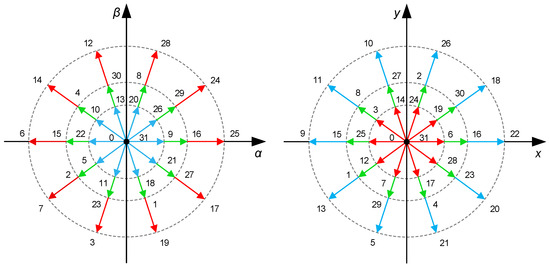
Figure 3.
Available voltage vectors in the αβ and xy subspaces, identified by the decimal number derived from the switching vector.

Table 1.
Induction machine used in our study.
3. Finite Control Set MPC in 5PIM Drives
Different predictive stator current control strategies can be applied to the 5pIM drive, which differ mainly in the system variables that are regulated and in the way control actions are applied. The finite control set MPC structure (FCS-MPC) selects the optimal control action that commands the 5p2L-VSI. An outer speed/torque PI-based controller, which is usually based on the conventional field-oriented control (FOC) strategy, needs to be added to provide current references to the FCS-MPC algorithm. These references are given in a rotating reference frame, called dq, for better regulation, where the reference of the q-current stator (isq*) is the output of a PI regulator, while the reference of the d-current (isd*) is set to its nominal value. Once the objective currents are defined, the FCS MPC selects one switching state from the 32 possibilities to follow those references. This selection is made by minimizing a cost function that compares the current references with a prediction made based on a mathematical model of the system: the prediction model. The basis of the predictive controller is then the optimal selection of the switching state of the power converter using a predictive model of the controlled system (a five-phase induction drive in our case).
An alternative way of implementing an MPC algorithm is the variable sampling time lead-pursuit controller or VSTLPC technique in what follows. The basis of this technique is the optimal selection of both the switching state of the power converter and its time of application between all possibilities without the necessity of a cost function. VSTLPC begins finding the optimal switching state from some measurements (rotor speed and stator currents) and applying the lead-pursuit concept: Hitting a moving target requires some anticipation, since it takes some time for the control action to produce an effect on the system, and during such time, the target changes its position. In this way, the controller points to an advanced stator current reference, and the switching vector that produces the trajectory of the stator currents to the reference is selected.
This work combines VSTLPC and the VVV concepts in the current control of the 5pIM drive to reduce harmonic distortion in machine currents and to improve the efficiency of the system (see Figure 4). Then, the outer speed loop is maintained while the control action is implemented using VSTLPC and considering different sets of VVV.
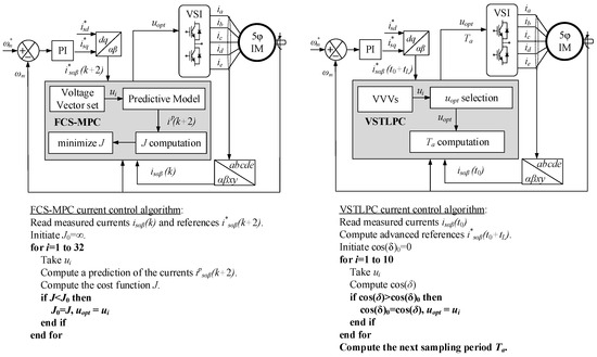
Figure 4.
Control schemes for a 5pIM drive using FCS-MPC (left side) and VSTLPC with VVV (right side) techniques.
3.1. Conventional VSTLPC Algorithm
The VSTLPC algorithm can be described as an innovative predictive control technique with the basic principle of giving freedom to the sampling time value of the predictive controller, i.e., applying variable sampling times. Then, the conventional VSTLPC controller deviates from FCS-MPC techniques, including a kind of modulation stage in the control stage [30]. The sampling time is selected from a limited number of possibilities together with the switching vector through a time-consuming optimization algorithm. Here, the basic idea presented in [30] is extended to the multiphase case and complemented by the lead-pursuit concept [31] to select the most adequate control action and its time of application with a finer resolution in the commuting times.
The inputs to the control algorithm are the measured stator currents and speeds and the current references imposed by the outer speed control loop. To anticipate the evolution of the currents, the references are advanced for a time tL, is*(t0 + tL). In the next step, 1 of the 32 possible VVs of the 5p2L-VSI, uopt = [vsα, vsβ, vsx, vsy], is selected by looking for the closest trajectory between the measured stator currents and the advanced references. First, the optimal trajectory is calculated as xs*(t0 + tL) − xs(t0), where xs = [isα isβ isx isy]. Then, the following maximization problem is solved:
where x = [isα isβ isx isy irα irβ], f(x, u) is a function that characterizes the evolution of the stator currents: f(x, u) = dxs/dt. δ is the angle between f(x(t0), ui) and the distance (x*(t0 + tL) − xs(t0)). This function is defined from Equation (3) and has four components, for which their values depend on the measured stator and rotor currents in the αβ plane and the measured rotor speed. Finally, the time during which the chosen VV must be applied, Ta, is calculated, as indicated in Equation (5). The formula is derived from an optimization problem where the deviation between the stator references and a prediction based on the system model is minimized.
3.2. Proposed VSTLPC Considering VVV as Control Actions
The incorporation of VVV as control actions in the FCS-MPC has permitted the improvement of current quality in multiphase drives, thanks to the simultaneous regulation of the available subspaces [29]. These vectors are created through a combination of two or more voltage vectors in such a way that zero or reduced average voltage amplitudes are produced in the xy plane. Consequently, the regulation of secondary currents is directly carried out with the VVV application, without including a specific control loop in the algorithm. This characteristic results in the simplification of the prediction model and the predictive control algorithm. In this work, diverse sets of 10 virtual VVVs are used in the optimization problem of the VSTLPC algorithm instead of the 32 original VVs of the 5p2L-VSI.
For the case under study, three sets of VVVs will be independently considered as control actions, with the objective of comparing the pros and cons of each one (Table 2 summarizes the sets of VVVs that will be considered in this work):
Table 2.
Set of VVVs considered.
Medium–large VV (ML-VVV): A large vector is combined with a medium vector with dwell ratios equal to λ1 = 0.382 and λ2 = 0.618, respectively. As seen in Figure 3, they are aligned in the αβ plane, but they are in the opposite direction in the xy plane (vectors 12 and 30, for example), and their combination leads to a VVV with zero xy voltage on average. This is the common strategy in most research, where a total of 10 VVVs can be constructed considering all possible combinations. As a disadvantage, the instantaneous value of the xy voltage components is not zero, thus producing the circulation of xy currents in the machine. Furthermore, the use of the DC link is reduced compared to the original voltage vectors, since the size of the VVV is 0.5528Vdc. The latest has an important influence on the operating range of the drive, mainly in high-speed/torque operation.
Duo of large VVs (LL-VVV): Two adjacent large voltages are combined with dwell times ratios equal to λ1 = λ2 = 0.5. In this case, the combination will not provide zero xy voltage amplitudes (see vectors 12 and 28, for example), but its magnitude is limited by applying the indicated dwell ratios. Therefore, secondary currents will not effectively be regulated to zero, but their instantaneous values will be lower than those with conventional VVVs. Additionally, the resulting VVV has a size of 0.6155Vdc in the primary plane, which extends the use of the DC link. As in the previous case, 10 different VVVs can be constructed.
Trio of large VVs (LLL-VVV): Three adjacent large vectors are combined with λ1 = 0.382, λ2 = 0.236, and λ3 = 0.382 as dwell ratios. In this case, zero-average xy voltages are obtained with low instantaneous xy injection, thus resulting in the expectation of improved current quality in the machine compared to the application of the medium–large combination. However, the magnitude of the new VVV is 0.5528Vdc, and the use of the DC link is poorer compared to the set of VVVs formed by only two adjacent voltage vectors.
Following the same algorithm described above, the VSTLPC selects the optimal VVV to be applied and its application time based on the measured currents and the established references. Only a set of VVVs and a zero vector are considered as possible control actions. In this case, the optimization problem used to choose the optimal control action, uopt = [vsα, vsβ], is reduced to the following:
At this point, the xy plane is not considered in the machine’s model due to the incorporation of VVV, so xαβ = [isα, isβ, irα, irβ] and xsαβ = [isα, isβ]; fαβ(xαβ, u) is a vector of two components for which their values depend on the measured stator currents in the αβ subspace, the αβ rotor currents, and the measured rotor speed. Afterwards, the time of application of the selected VVV is obtained using Equation (7). Note that the dwell ratios of the corresponding VVVs must be used to define the 5p2L-VSI switching sequence, and the described algorithm is valid for any VVV group.
4. Results and Discussion
The effectiveness and efficiency of the proposed controller are explored, and the sets of VVVs are detailed in Table 2. Note that the selection of the parameters used in the experiments is based on heuristic adjustment and empirical observation. In all tests, maximum and minimum values are imposed for the sampling time Ta to consider limitations in the efficiency of the control algorithm and in the 5p2L-VSI switching frequency. In our case, the maximum value is set at 150 µs, while the minimum value is forced to be 32.5 µs using the conventional VSTLPC method and the proposed controller, and the advanced time tL is set to Tamin. A group of tests was conducted to compare the performance in the steady state of the original VSTLPC and the proposed one once the machine was close to the achievable limits. Figure 5, Figure 6, Figure 7 and Figure 8 summarize the results obtained.
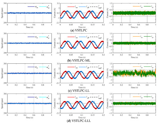
Figure 5.
Steady-state response at 300 rpm and 50% of the nominal torque using conventional VSTPLC (a) and the proposed controller with ML-VVV (b), LL-VVV (c), and LLL-VVV (d). From left to right: mechanical speed and αβ and xy stator currents.
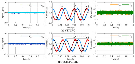
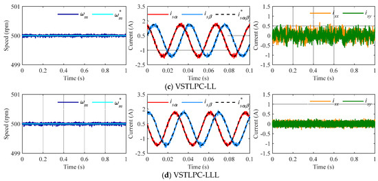
Figure 6.
Steady-state response at 500 rpm and 85% of the nominal torque using conventional VSTPLC (a) and the proposed controller with ML-VVV (b), LL-VVV (c), and LLL-VVV (d). From left to right: mechanical speed and αβ and xy stator currents.
Figure 7.
Steady-state response at 600 rpm and 85% of the nominal torque using the proposed controller with ML-VVV (a), LL-VVV (b), and LLL-VVV (c). From top to bottom: mechanical speed and αβ, xy, and dq stator currents.
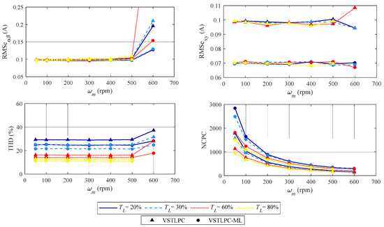
Figure 8.
Obtained figure of merits in different operating points (reference speed and load torque) using the conventional VSTLPC technique and the proposed control method with ML-VVV.
In the first experiment (see Figure 5), a reference speed of 300 rpm (ωm) is imposed, and a load torque (TL) equal to 50% of the nominal is applied. The regulation of speed and the control of the stator current in the αβ plane are achieved effectively in all cases. However, interesting comments regarding the stator current’s performance in the xy subspace must be made. Considering VSTLPC with virtual ML and LLL vectors, a reduction in the xy current components is observed relative to the original VSTLPC technique. This leads to a reduction in the harmonic content of the stator currents and, consequently, to a higher system efficiency, thanks to the use of virtual voltage vectors themselves, which produce an effective open-loop regulation of the xy plane. However, a different situation is observed with the LL virtual vectors, where a non-zero-average xy voltage is imposed and higher xy stator current components appear, as expected. A reference speed of 500 rpm (ωm) is imposed, and a load torque (TL) equal to 85% of the nominal is applied in a second batch of tests (see Figure 6). Again, the regulation of speed and control of the stator current in the αβ plane are achieved effectively in all cases, and the main conclusions achieved in the first experiment are confirmed.
A second batch of experiments is then considered, where higher speed and torque conditions are imposed, and the optimal usage of the DC link voltage becomes essential. Figure 7 shows the results obtained when a speed reference of 600 rpm and 85% of the nominal torque is forced. In this case, VSTLPC with ML and LL-VVV is not capable of effectively controlling the machine’s speed. This is the main consequence of their limited DC link utilization because of the reduced magnitude of these VVVs. This situation produces the saturation of the q-current reference generated by the PI regulator, which achieves the maximum admissible value. In contrast, when LL-VVV vectors are applied, the speed can be regulated because of the extended DC link utilization provided by this set of virtual vectors, at the expense of suboptimal current quality. Then, LL-VVV provides higher voltage magnitudes compared to other virtual vector groups.
Several merit figures have been depicted to perform a comparative analysis in terms of the efficiency of the system’s performance at different operating points, comparing the proposed controller and the conventional VSTLPC. Again, different sets of VVVs are used to extend the exhaustiveness of the analysis. The merit figures obtained include the number of switching commutations per cycle (NCPC), the root mean square error in the current tracking for the αβ plane (RMSαβ), the root mean square error in the current tracking for the plane xy (RMSxy), and the total harmonic distortion of the currents (THD), which are defined as follows:
The original VSTLP controller is compared with the proposal using ML-VVV, since LLL-VVV provides similar results and our interest in LL-VVV is limited to high-speed/torque demanding operations. Figure 8 summarizes the results obtained. Regardless of the speed and torque demand, the proposed controller provides lower harmonic distortions in the stator currents due to the reduction in the xy stator voltage components (lower RMSxy values). In contrast, there are no important differences in the regulation of torque and flux, except in high-speed operations. Note that NCPC increases significantly in the proposed controller with the application of the VVV concept. This is a direct consequence of using VVV and two switching states of the 5p2L-VSI in the same sampling period, while only one switching state is applied in the case of the original VSTPLC method. This result can generate a disadvantage when using the proposed controller because it can force an increase in the switching losses of the power converter.
Therefore, incorporating VVVs into the VSTLPC algorithm can improve the efficiency of the controlled system, reducing copper losses by limiting the injection of the xy current. This is the case when ML-VVV or LLL-VVV is considered. This improvement is also complemented by a reduction in the computational burden of the controller due to the simplification of the predictive model using the VSTLPC algorithm. However, the use of two or three voltage vectors in a sampling period instead of only one can increase the switching losses in the power converter, limiting the interest of the proposal. Note also that the use of VVV leads to a reduction in DC link voltage utilization, which limits the operating range of the machine. This drawback can be mitigated using LL-VVV, which extends the operational range in the real system compared to using ML-VVV or LLL-VVV. As a general conclusion, the selection of the applied VVV should be carried out based on the required control performance and the operational point of the machine.
5. Conclusions
Predictive current controllers have been recently proposed as an interesting control technique in multidimensional and nonlinear systems like multiphase IM drives. This control technique offers remarkable benefits, but some disadvantages appear, which can be summarized in the high computational cost and the generation of higher harmonic stator current components. This work combines the lead-pursuit strategy and the virtual voltage vector concepts to mitigate both disadvantages in predictive controllers. Three sets of VVVs are considered with the lead-pursuit method in our study, but alternatively, different sets should be analyzed to improve the quality of the analysis. The proposal has been analyzed on a five-phase IM drive testing platform to state its interest and viability. The results obtained highlight that the selection of the set of VVVs utilized is important to improve the stator current, electrical torque, and speed regulations and should vary depending on the control reference to extend the benefits of the proposal throughout the operating range of the drive. They are also important for quantifying the performance of the closed-loop system in terms of some predefined merit figures: in our case, the number of switching commutations per cycle, the root mean square error in the current tracking, and the total harmonic distortion of the stator current. Although the proposal was properly analyzed on a specific multiphase induction machine, further work should be carried out to indicate its actual interest. The authors consider that the proposal should also be extended to permanent magnet or synchronous resistance machines and MCT switches, among other technologies of electric drives, and that it should be extended to electrical drives with different numbers of phases, thereby spreading the interest in lead-pursuit-based predictive control methods.
Author Contributions
Conceptualization, F.B., M.B., M.R.A. and I.G.-P.; methodology, F.B., M.B., M.R.A. and I.G.-P.; software, M.B.; validation, F.B., M.B., M.R.A. and I.G.-P.; formal analysis, F.B., M.B., M.R.A. and I.G.-P.; investigation, F.B., M.B., M.R.A. and I.G.-P.; resources, F.B., M.B., M.R.A. and I.G.-P.; data curation, M.B.; writing—original draft preparation, F.B.; writing—review and editing, F.B., M.B., M.R.A. and I.G.-P.; visualization, F.B., M.B., M.R.A. and I.G.-P.; supervision, F.B.; project administration, F.B.; funding acquisition, F.B. All authors have read and agreed to the published version of the manuscript.
Funding
This research was funded by the Grant TED2021-129558B-C22 funded by MCIU/AEI/10. 13039/501100011033 and by the “European Union NextGenerationEU/PRTR” and the project I+D+i/PID2021-125189OB-I00, funded by MCIU/AEI/10.13039/501100011033/ by “ERDF A way of making Europe”.
Institutional Review Board Statement
Not applicable.
Informed Consent Statement
Not applicable.
Data Availability Statement
The original contributions presented in this study are included in the article. Further inquiries can be directed to the corresponding author.
Conflicts of Interest
The authors declare no conflicts of interest.
References
- Liu, C. Emerging Electric Machines and Drives—An Overview. IEEE Trans. Energy Convers. 2018, 33, 2270–2280. [Google Scholar] [CrossRef]
- Linder, A.; Kanchan, R.; Stolze, P.; Kennel, R. Model-Based Predictive Control of Electric Drives; Cuvillier Verlag Göttingen: Springer London, Germany, 2010. [Google Scholar]
- Rathore, V.; Yadav, K. Efficiency analysis of six-phase induction motor drive using an optimized SVM technique for medium/high power applications. Optim. Control. Appl. Methods 2023, 44, 3237–3256. [Google Scholar] [CrossRef]
- Slunjski, M.; Dordevic, O.; Jones, M.; Levi, E. Symmetrical/asymmetrical winding reconfiguration in multiphase machines. IEEE Access 2020, 8, 835–844. [Google Scholar] [CrossRef]
- Rigatos, G.; Cuccurullo, G.; Siano, P.; Abbaszadeh, M. Nonlinear optimal control for VSI-fed six-phase PMSMs. AIP Conf. Proc. 2023, 2849, 180003. [Google Scholar]
- Camacho, E.F.; Bordons, C. Model Predictive Control, 2nd ed.; Springer: Berlin/Heidelberg, Germany, 2007. [Google Scholar]
- Geyer, T. Model Predictive Control of High Power Converters and Industrial Drives; John Wiley and Sons: Hoboken, NJ, USA, 2016. [Google Scholar]
- Tenconi, A.; Rubino, S.; Bojoi, R. Model Predictive Control for Multiphase Motor Drives—A Technology Status Review. In Proceedings of the International Power Electronics Conference (IPEC), Niigata, Japan, 20–24 May 2018; pp. 732–739. [Google Scholar]
- Karamanakos, P.; Liegmann, E.; Geyer, T.; Kennel, R. Model Predictive Control of Power Electronic Systems: Methods, Results, and Challenges. IEEE Open J. Ind. Appl. 2020, 1, 95–114. [Google Scholar] [CrossRef]
- Rodríguez, J.; Garcia, J.; Mora, A.; Flores-Bahamonde, F.; Acuna, P.; Novak, M. Department of Electrical Engineering, Universidad de Talca, Curico, Chile Cortes, P. Latest Advances of Model Predictive Control in Electrical Drives—Part I: Basic Concepts and Advanced Strategies. IEEE Trans. Power Electron. 2022, 37, 3927–3942. [Google Scholar] [CrossRef]
- Rodriguez, J.; Cortes, P. Latest Advances of Model Predictive Control in Electrical Drives—Part II: Applications and Benchmarking with Classical Control Methods. IEEE Trans. Power Electron. 2022, 37, 5047–5061. [Google Scholar] [CrossRef]
- Choi, Y.; Lee, W.; Kim, J.; Yoo, J. A Variable-Sampling Time Model Predictive Control Algorithm for Improving Path-Tracking Performance of a Vehicle. Sensors 2021, 21, 6845. [Google Scholar] [CrossRef]
- Mamdouh, M.; Abido, M.A. Simple predictive current control of asymmetrical six-phase induction motor with improved performance. IEEE Trans. Ind. Electron. 2022, 70, 7580–7590. [Google Scholar] [CrossRef]
- Arahal, M.R.; Barrero, F.; Satué, M.G.; Bermúdez, M. Fast Finite-State Predictive Current Control of Electric Drives. IEEE Access 2023, 11, 12821–12828. [Google Scholar] [CrossRef]
- Li, T.; Sun, X.; Lei, G.; Yang, Z.; Guo, Y.; Zhu, J. Finite-control-set model predictive control of permanent magnet synchronous motor drive systems—An overview. IEEE/CAA J. Autom. Sin. 2022, 9, 2087–2105. [Google Scholar] [CrossRef]
- Yu, B.; Song, W.; Li, J.; Li, B.; Saeed, M.S. Improved finite control set model predictive current control for five-phase VSIs. IEEE Trans. Power Electron. 2020, 36, 7038–7048. [Google Scholar] [CrossRef]
- Arahal, M.R.; Barrero, F.; Satue, M.G.; Martin, C.; Bermudez, M. Evolutionary Gaps Stator Current Control of Multiphase Drives Balancing Harmonic Content. IEEE Trans. Ind. Electron. 2024, 71, 6886–6893. [Google Scholar] [CrossRef]
- Song, X.; Wang, H.; Ma, X.; Yuan, X.; Wu, X. Robust model predictive current control for a nine-phase open-end winding PMSM with high computational efficiency. IEEE Trans. Power Electron. 2023, 38, 13933–13943. [Google Scholar] [CrossRef]
- Serra, J.; Jlassi, I.; Cardoso, A.J.M. A computationally efficient model predictive control of six-phase induction machines based on deadbeat control. Machines 2021, 9, 306. [Google Scholar] [CrossRef]
- Arahal, M.R.; Barrero, F.; Duran, M.J.; Martin, C. Harmonic Distribution in Finite State Model Predictive Control. Int. Rev. Electr. Eng. 2015, 10, 172–179. [Google Scholar] [CrossRef]
- De Abreu, J.P.G.; Emanuel, A. The need to limit subharmonics injection. In Proceedings of the 9th International Conference on Harmonics and Quality of Power, Orlando, FL, USA, 1–4 October 2000; Volume 1, pp. 251–253. [Google Scholar] [CrossRef]
- Gnacinski, P.; Peplinski, M.; Szweda, M. The effect of subharmonics on induction machine heating. In Proceedings of the 13th Power Electronics and Motion Control Conference (EPE-PEMC 2008), Poznań, Poland, 1–3 September 2008; pp. 826–829. [Google Scholar] [CrossRef]
- Barrero, F.; Arahal, M.R.; Gregor, R.; Toral, S.; Duran, M.J. One-step modulation predictive current control method for the asymmetrical dual three-phase induction machine. IEEE Trans. Ind. Electron. 2009, 56, 1974–1983. [Google Scholar] [CrossRef]
- Gonzalez, O.; Ayala, M.; Rodas, J.; Gregor, R.; Rivas, G.; Doval-Gandoy, J. Variable-speed control of a six-phase induction machine using predictive-fixed switching frequency current control techniques. In Proceedings of the 9th IEEE International Symposium on Power Electronics for Distributed Generation Systems (PEDG-2018), Charlotte, NC, USA, 25–28 June 2018; pp. 1–6. [Google Scholar]
- Duran, M.J.; Gonzalez-Prieto, I.; Gonzalez-Prieto, A. Large virtual voltage vectors for direct controllers in six-phase electric drives. Int. J. Electr. Power 2021, 125, 106425. [Google Scholar] [CrossRef]
- Gonzalez-Prieto, I.; Duran, M.J.; Aciego, J.J.; Martin, C.; Barrero, F. Model predictive control of six-phase induction motor drives using virtual voltage vectors. IEEE Trans. Ind. Electron. 2018, 65, 27–37. [Google Scholar] [CrossRef]
- Arahal, M.R.; Martín, C.; Barrero, F.; Durán, M.J. Assessing Variable Sampling Time Controllers for Five-Phase Induction Motor Drives. IEEE Trans. Ind. Electron. 2020, 67, 2523–2531. [Google Scholar] [CrossRef]
- Soto-Marchena, D.; Barrero, F.; Colodro, F.; Arahal, M.R.; Mora, J.L. On-Site Calibration of an Electric Drive: A Case Study Using a Multiphase System. Sensors 2023, 23, 7317. [Google Scholar] [CrossRef] [PubMed]
- Bermúdez, M.; Martín, C.; González-Prieto, I.; Durán, M.J.; Arahal, M.R.; Barrero, F. Predictive current control in electrical drives: An illustrated review with case examples using a five-phase induction motor drive with distributed windings. IET Electr. Power App. 2020, 14, 1291–1310. [Google Scholar] [CrossRef]
- Hoffmann, N.; Andresen, M.; Fuchs, F.W.; Asiminoaei, L.; Thøgersen, P.B. Variable sampling time finite control-set model predictive current control for voltage source inverters. In Proceedings of the IEEE Energy Conversion Congress and Exposition (ECCE-2012), Raleigh, NC, USA, 15–20 September 2012; pp. 2215–2222. [Google Scholar]
- Isaacs, R. Differential games: A Mathematical Theory with Applications to Warfare and Pursuit, Control and Optimization; Courier Corporation: North Chelmsford, MA, USA, 1999. [Google Scholar]
Disclaimer/Publisher’s Note: The statements, opinions and data contained in all publications are solely those of the individual author(s) and contributor(s) and not of MDPI and/or the editor(s). MDPI and/or the editor(s) disclaim responsibility for any injury to people or property resulting from any ideas, methods, instructions or products referred to in the content. |
© 2025 by the authors. Licensee MDPI, Basel, Switzerland. This article is an open access article distributed under the terms and conditions of the Creative Commons Attribution (CC BY) license (https://creativecommons.org/licenses/by/4.0/).