Optimization Configuration Method for Grid-Forming and Grid-Following Energy Storage Based on Node Frequency Deviation Coefficient

Abstract

As the power system develops towards a high proportion of renewable energy sources and power electronic devices, the power system suffers from poor frequency stability due to the lack of synthetic inertia. The grid-forming energy storage can not only improve the frequency dynamic response of the generator and enhance inertia support capability but can also realize the peak regulation and valley filling of the power system. But its relatively high configuration cost restricts its development and construction. Therefore, how to rationally configure the grid-forming energy storage and grid-following energy storage within the power system by means of corresponding technical approaches has become the focal point of academic research. This study proposes a method for evaluating the inertia distribution characteristics of the power system based on the network equations of the power system. Furthermore, the demand for grid-forming energy storage at each node of the power system under different operation scenarios can be quantified according to this method. Finally, an optimization configuration method for an energy storage system that can improve the inertia distribution characteristics of the power system is proposed, and its effectiveness is verified through the 39-bus system.

1. Introduction

An increasing number of renewable energy sources (RESs) represented by wind and photovoltaic power are connected to the power grid. They are gradually replacing synchronous generators (SGs) and emerging as the predominant power sources in the renewable energy power system [1,2]. RESs are connected to the power system through power electronic devices and are unable to provide inherent inertia [3,4]. Moreover, the power output of RESs can be influenced by various factors, such as weather conditions, geographical locations, and control strategies [5]. Consequently, in the context of power disturbance events, the issues of fluctuations and uncertainties within the power system become more conspicuous, thereby affecting the frequency regulation capabilities of RESs, which are characterized by variations over time and across different locations [6]. Due to the low inertia and uncertainties of the power system, the frequency response of the power system deteriorates, the frequency regulation ability of RES exhibits distribution characteristics [7], and the increased rate of change of frequency (RoCoF) at some nodes poses a challenge to the secure operation of the grid.

Compared with SGs, power electronic devices can achieve power control within a smaller time scale [8]. They have broad application prospects in RESs. At the same time, with the features of bidirectional transmission and rapid response [9], an energy storage system (ESS) is likely to exert a significant influence in the renewable energy power system. Therefore, ESSs can serve as an effective means to improve the stable operation of the power grid. The control methods used in ESSs can be categorized into grid-following (GFL) control and grid-forming (GFM) control [10,11,12]. Regarding the improvement of the secure operation capacity of the power system, techniques of applying GFM technology within low-inertia power systems have garnered substantial research attention.

Many efforts have already been made by scholars in researching the evaluation methods of the inertia distribution characteristics of power systems. The authors of [13] propose a method to quantify estimation frequency characteristics to reflect the differences in the inertia support capability of various nodes. The frequency responses of each node in the power system under various inertia distribution characteristics were analyzed via simulation in [14]. In large-scale power systems, a variety of inertia distribution indexes are proposed to describe the impact of inertia on the frequency stability of the power systems [15,16]. Quantitative assessment of power system inertia allocation can be made through trajectory analysis of electromechanical disturbance propagation [17].

In recent years, with the continuous development of GFM control strategies, extensive research has been conducted on the application of grid-forming control energy storage systems (GFM-ESSs) to enhance the secure and stable operation of renewable energy power systems. GFM control can effectively enhance the stability of the power system and is expected to solve the problem that the replacement of SGs by RESs leads to a significant decline in the inertia of the power system [18,19]. An RES production forecasting method using artificial neural networks was proposed in [20]. This method exhibits a lower mean average prediction error and provides more accurate evaluation results. Regarding the configuration method of GFM-ESSs, the authors in [21] establish a frequency response model of the wind-energy storage system and achieve the allocation of virtual inertia between wind power and ESSs according to the inertia requirements of the system. A site selection and capacity optimization method was designed from the perspective of reactive-voltage sensitivity calculation in [22]. Based on multiple time scales, a plant siting and capacity optimization method for GFM-ESSs that can enhance the inertia of the power system and the cycle life of ESSs was proposed in [23]. Considering various scenarios of major power outages, a parallel restoration strategy utilizing the A* algorithm was proposed in [24], which can provide reliable power supply to consumers.

While GFM-ESSs have the ability to provide inertia to a power system, the configuration cost of GFM-ESSs is notably higher compared with grid-following energy storage systems (GFL-ESSs). Furthermore, GFM-ESSs share similar functions with GFL-ESSs in terms of power balancing and peak load regulation. Most of the existing studies focus on the capacity planning or the optimization of control strategies for a single type of ESS, making it a critical issue to study the capacity ratio between GFM-ESSs and GFL-ESSs.

Inspired by the above-mentioned research, a hybrid optimization method is proposed for the coupled placement and capacity allocation of GFM-ESS and GFL-ESS construction. This method, which is applicable to the field of power system planning, addresses the problem of utilizing the minimum amount of GFM-ESSs to solve the issue of insufficient inertia support capability in power systems, thereby enabling the stable operation of a renewable energy power system. The main advancements are delineated as follows:

Based on the network equations of a power system, this study presents a method for evaluating the inertia support capability of generators in the power system. A virtual inertia emulation framework is subsequently formulated for GFM-ESSs, explicitly integrating frequency dynamics characteristics. Taking the integration of RESs into account, the frequency relationship between the generators and the network nodes is deduced, and according to the frequency relationship, the inertia distribution characteristics of the power system are characterized by using the node frequency regulation coefficient. Furthermore, a method for the optimization configuration of ESSs considering the inertia distribution characteristics of the power system is proposed. This method, which can quantify the configuration requirements of GFM-ESSs, aims to enhance the inertia support capacity of generator nodes and reduce the operation cost of the power system. In summary, the major contributions of this study are mainly reflected in two aspects: (1) the method for evaluating the inertia distribution characteristics considering the grid structure of a power system and (2) an optimization configuration method for site selection and capacity determination of GFL-ESSs and GFM-ESSs considering inertia distribution characteristics.

The remainder of this study is structured as follows: Section 2 assesses the inertia support capability of different generator nodes in the power system using network equations and introduces a method to characterize the distribution of inertia resources in the system. Section 3 evaluates the demand for GFM-ESSs in the power system and designs an optimization configuration method for ESSs based on multiple operation scenarios. Section 4 verifies the effectiveness of the evaluation method and the proposed configuration method on the IEEE 9-bus system and IEEE 39-bus system, respectively. Section 5 provides a summary of this study.

2. Evaluation Method of Inertia Distribution Characteristics

When the power system experiences a large disturbance, the inertia of generators helps to stabilize the frequency and prevent its deviation. The synthetic inertia includes the rotational inertia of SGs and the frequency support of RESs and ESSs through the power electronic devices. Due to the differences in inertia support capability of generators, the key features of frequency dynamic process including RoCoF and frequency nadir are significantly different, and these can be described as inertia distribution characteristics. Considering the network equation of power systems, an evaluation method for inertia which can evaluate the inertia level of generators in the power system is proposed in this section. Compared with SGs, the mode of GFM-ESSs participating in the frequency dynamic process is different. In this section, inertia response model of GFM-ESSs will also be established.

2.1. Inertia Response Model of GFM-ESS

A GFM-ESS primarily consists of energy storage elements, power conversion system, and GFM converter. The control strategy of converter utilizes virtual synchronous machine (VSM) control [25], which encompasses the virtual governor, the rotational rotor equation, the virtual excitation regulator, and the stator electrical equation. The topology and control diagram of the GFM-ESS is shown in Figure 1.

The VSM control emulates the governor’s external characteristics by establishing droop characteristics between active power and system frequency, which can be expressed as Equations (1) and (2).

$$P_{\mathrm{m}}=P_{\mathrm{ref}}+\Delta P=P_{\mathrm{ref}}+k_{\mathrm{p}}({\omega }_{\mathrm{ref}}-{\omega }_{\mathrm{grid}})$$

(1)

$$\left\{\begin{array}{l}J{\displaystyle \frac{\mathrm{d}\left(\omega -{\omega }_{\mathrm{ref}}\right)}{\mathrm{d}t}}={\displaystyle \frac{P_{\mathrm{m}}}{{\omega }_{\mathrm{ref}}}}-{\displaystyle \frac{P_{\mathrm{e}}}{{\omega }_{\mathrm{ref}}}}-D\left(\omega -{\omega }_{\mathrm{ref}}\right)\hfill \\ {\displaystyle \frac{\mathrm{d}\delta }{\mathrm{d}t}}=\omega -{\omega }_{\mathrm{ref}}\hfill \end{array}\right.$$

(2)

where ${\omega }_{\mathrm{ref}}$ and ${\omega }_{\mathrm{grid}}$ represent the rated and actual angular velocities of the power system, $k_{\mathrm{p}}$ denotes the droop coefficient, and $P_{\mathrm{m}}$ and $P_{\mathrm{ref}}$ correspond to the mechanical power and reference active power.

Equation (3) represents the reactive power control loop, which generates the reference internal voltage by simulating the excitation mechanism of SG.

$$\left\{\begin{array}{l}E=E_0+k_{\mathrm{qi}}\Delta Q/s+k_{\mathrm{v}}\Delta U\\ \Delta Q=Q_{\mathrm{ref}}-Q\\ \Delta U=U_{\mathrm{ref}}-U\end{array}\right.$$

(3)

where $k_{\mathrm{v}}$ represents the reactive voltage proportional coefficient, $k_{\mathrm{qi}}$ denotes the reactive power integral coefficient, $E$ corresponds to the internal voltage, $\Delta Q$ represents the reactive power change, $U_{\mathrm{ref}}$ represents the voltage of point of common coupling (PCC), $\Delta U$ represents the deviation of voltage, and $E_0$ signifies the no-load electromotive force.

The GFM-ESS implements frequency regulation in power systems through the active power–frequency control loop depicted in Figure 2, where $k_{\mathrm{f}}$ denotes the active droop coefficient, $J$ represents the virtual inertia coefficient determining inertial response characteristics, and $D$ represents the damping coefficient.

2.2. Inertia Evaluation Method Based on Node Frequency Deviation Coefficient (NFDC)

By analyzing the load flow calculation results during the operation of the power system, the active power output of each generator throughout the operation process is determined.

$$P_i=U_i{\displaystyle \sum _{j=1}^n{U}_j}(G_{ij}\cos {\delta }_{ij}+B_{ij}\sin {\delta }_{ij})$$

(4)

where $P_i$ represents the active power output of the generator, $U_i$ and $U_j$ represent the voltage magnitudes, $G_{ij}$ and $B_{ij}$ denote the equivalent impedance and admittance, and ${\delta }_{ij}$ represents the phase difference.

For a power system incorporating RESs, the mathematical relationship is as shown in Equation (5). G, L, and R represent the generators, loads, and grid nodes in the power system. Y can describe the connection relationships between the various nodes in the power system, which is composed of admittances.

$$I=\left[\begin{array}{c}{I}_G\\ I_L\\ I_R\end{array}\right]=\left[\begin{array}{ccc}{Y}_{GG}& Y_{GL}& Y_{GR}\\ Y_{LG}& Y_{LL}& Y_{LR}\\ Y_{RG}& Y_{RL}& Y_{RR}\end{array}\right]\left[\begin{array}{c}{U}_G\\ U_L\\ U_R\end{array}\right]$$

(5)

Since the network nodes are considered passive nodes, the node current at these nodes can be approximated as zero. Therefore, the network equation of power system can be expressed as Equation (6).

$$\left[\begin{array}{c}{I}_G\\ I_L\\ 0\end{array}\right]=\left[\begin{array}{ccc}{Y}_{GG}& Y_{GL}& Y_{GR}\\ Y_{LG}& Y_{LL}& Y_{LR}\\ Y_{RG}& Y_{RL}& Y_{RR}\end{array}\right]\left[\begin{array}{c}{U}_G\\ U_L\\ U_R\end{array}\right]$$

(6)

According to network equation, the relationship between the voltage of each node in power system can be shown in Equation (7).

$$Y_{RG}{U}_G+Y_{RL}{U}_L+Y_{RR}{U}_R=0$$

(7)

$$-Y_{RR}^{-1}\left[\begin{array}{cc}{Y}_{RG}& Y_{RL}\end{array}\right]\left[\begin{array}{c}{U}_G\\ U_L\end{array}\right]=U_R$$

(8)

When a disturbance occurs in the system, the node voltage of power system typically undergoes only minor changes. By differentiating the voltage phase in Equation (8), the following relationship can be obtained as in Equations (9) and (10).

$$Y_{\mathrm{eq}}{V}_G{\displaystyle \frac{\mathrm{d}{\delta }_G}{\mathrm{d}t}}=V_R{\displaystyle \frac{\mathrm{d}{\delta }_R}{\mathrm{d}t}}$$

(9)

$$Y_{\mathrm{eq}}=-Y_{RR}^{-1}\left[\begin{array}{cc}{Y}_{RG}& Y_{RL}\end{array}\right]$$

(10)

The per-unit value of node voltage in the power system is usually approximately equal to 1, so the frequency relationship between the network nodes and generators is shown in Equation (11).

$$f_R=Y_{\mathrm{eq}}{f}_G$$

(11)

By differentiating both sides of Equation (10) with respect to frequency, the relationship between the RoCoF of each node of the power system can be derived as in Equation (12).

$${\displaystyle \frac{\mathrm{d}{f}_R}{\mathrm{d}t}}=Y_{\mathrm{eq}}{\displaystyle \frac{\mathrm{d}{f}_G}{\mathrm{d}t}}$$

(12)

The frequency responses of generators in the power system are represented by rotational motion equation, as shown in Equation (13).

$$\left\{\begin{array}{l}{K}_J{\displaystyle \frac{\mathrm{d}{f}_G}{\mathrm{d}t}}=-\Delta P_G\hfill \\ {\displaystyle \frac{\mathrm{d}{\delta }_G}{\mathrm{d}t}}=f_G\hfill \end{array}\right.$$

(13)

The relationship between the frequency response and the active power output of power system can be clearly determined as in Equation (14).

$${\displaystyle \frac{\mathrm{d}{f}_R}{\mathrm{d}t}}=Y_{\mathrm{eq}}{K}_J^{-1}\Delta P_G$$

(14)

where $K_J$ is the matrix composed of the inertia time constants of the generator nodes, and $\Delta P_G$ represents the active power change of power system.

$$\left\{\begin{array}{l}{\displaystyle \frac{\mathrm{d}{f}_{\mathrm{Ri}}}{\mathrm{d}t}}={\displaystyle \sum _{j=1,j\ne i}^n{M}_{ij}^{\mathrm{eq}}}\Delta {\delta }_{ij}\\ M_{ij}^{\mathrm{eq}}={\displaystyle \sum _{i=1}^n\frac{Y_{\mathrm{eq}}^{m,r}}{K_{Ji}}\Delta P_G}\end{array}\right.$$

(15)

where $M_{ij}^{\mathrm{eq}}$ represents the node frequency regulation coefficients, n denotes the number of generators in the power system, and $\mathrm{d}{f}_{Ri}/\mathrm{d}t$ indicates the frequency variation rate. The matrix $M$ reflects the relationship between the frequency responses of the various generators. Equation (15) shows that when a power disturbance event occurs, the inertia support capability of different nodes can be influenced by inertia distribution characteristics and grid structure of the power system.

Based on Equation (15), if a power disturbance occurs at a certain node in the system, the node frequency deviation coefficient (NFDC) for that node can be derived as in Equation (16).

$$NFD{C}_k={\displaystyle \sum _{j=1,j\ne i}^n{M}_{ij}^{\mathrm{eq}}}$$

(16)

3. Optimization Configuration Method of ESS

In the optimization configuration method for energy storage capacity and location selection, the value of NFDC can be utilized to evaluate the inertia distribution characteristics of power system. Subsequently, the stability operating boundaries of the power system are designed according to relevant standards. It is assumed that the frequency in the power system is regulated by generators and ESSs. Based on the characteristics of RESs and loads in different seasons, the optimization objective is set to minimize the construction cost of ESSs and the operation cost of generators.

3.1. ESS Planning Formulation

In the optimization configuration model, the objective function proposed includes the operating cost of generators, the construction cost of ESSs, and the penalty cost of RESs. The specific expression is shown in Equations (17) and (18).

$$C_{\mathrm{con}}^{\mathrm{total}}=C_{\mathrm{SG}}^t+C_{\mathrm{res}}^t+C_{\mathrm{ess}}^t$$

(17)

$$\left\{\begin{array}{l}{C}_{\mathrm{SG}}^t={\displaystyle \sum _{i=1}^{N_{\mathrm{SG}}}{a}_m{(P_{\mathrm{SG},t}^i)}^2+b_m{P}_{\mathrm{SG},t}^i+c_m)}\\ C_{\mathrm{res}}^t={\displaystyle \sum _{i=1}^{N_{\mathrm{res}}}{c}_{i,\mathrm{res}}^{\mathrm{re}}(P_{i,\mathrm{res}}^{\mathrm{f}}-}{P}_{i,\mathrm{res}}^{\mathrm{r}})\\ C_{\mathrm{ess}}^t=({\displaystyle \sum _{i=1}^{N_{\mathrm{ess}}^{\mathrm{GFL}}}{k}_{\mathrm{GFL}}^{\mathrm{p}}\ast P_{\mathrm{GFL}}^{\mathrm{e}}+{\displaystyle \sum _{i=1}^{N_{\mathrm{ess}}^{\mathrm{GFM}}}{k}_{\mathrm{GFM}}^{\mathrm{p}}\ast P_{\mathrm{GFM}}^{\mathrm{e}})\ast \frac{r{(1+r)}^n}{{(1+r)}^n-1}}}\end{array}\right.$$

(18)

In the power system, $C_{\mathrm{SG}}^t$ represents the operational expenditure of conventional SGs; $C_{\mathrm{res}}^t$ is the penalty charges of RESs, which is designed to maximize the utilization efficiency of renewable energy; $C_{i,\mathrm{res}}^{\mathrm{re}}$ is the penalty coefficient of RESs; $N_{\mathrm{SG}}$ is the quantity of conventional SGs; $N_{\mathrm{res}}$ is the quantity of RESs; $a_m, b_m, c_m$ is the power generation cost coefficient of conventional SGs; $P_{\mathrm{SG},t}^i$ is the active power output of conventional SGs; $P_{i,\mathrm{res}}^{\mathrm{f}}$ and $P_{i,\mathrm{res}}^{\mathrm{r}}$ are the predicted output and actual output of RESs; $P_{\mathrm{GFL}}^{\mathrm{e}}$ and $P_{\mathrm{GFM}}^{\mathrm{e}}$, respectively, represent the power capacity of GFL-ESSs and GFM-ESSs; $k_{\mathrm{GFL}}^{\mathrm{p}}$ represents the cost coefficient of GFL-ESSs; $k_{\mathrm{GFM}}^{\mathrm{p}}$ represents the cost coefficient of GFM-ESSs; $r$ is the benchmark discount rate; and $n$ is the operational life of ESS.

3.2. Constraint Formulation

It is essential to configure GFM-ESSs due to the uneven distribution of inertia resources in the renewable energy power system. The NFDC is used to describe the frequency response ability of certain generators and the inertia distribution characteristics of power system. The value of NFDC is subject to the following constraint, which is shown in Equation (19).

$$NFD{C}_{\min }<(NFD{C}_i^{\mathrm{eq}}={\displaystyle \sum _{i=1}^{N_{\mathrm{G}}}\frac{Y_{\mathrm{eq}}^{m,r}}{K_{Ji}})<}NFD{C}_{\max }$$

(19)

where the quantity of generators in the power system is represented by $N_G$, and $NFD{C}_{\min }$ and $NFD{C}_{\max }$ are the extreme values of the system frequency change rate which can be determined according to relevant specifications for the stable operation of the power system.

According to the inertia constraint in Equation (19), the configuration requirements of GFM-ESSs can be clarified. It is feasible to guarantee that the frequency variation of the power system will remain within the safe operation range.

$${\displaystyle \sum K_J}=K_J(\mathrm{SG})+K_J(\mathrm{ESS})>{\displaystyle \sum Y_{\mathrm{eq}}^{m,r}}/NFD{C}_{\max }$$

(20)

The feasible region of ESS is subjected to a variety of constraints as shown in Equations (21)–(25), including capacity constraints and charge–discharge constraints.

$${\gamma }_{\mathrm{SOC}}{E}_{i,\mathrm{ess}}^{\min }\le E_{i,\mathrm{ess}}\le \left(1-{\gamma }_{\mathrm{SOC}}\right)E_{i,\mathrm{ess}}^{\max }$$

(21)

$$E_{i,\mathrm{ess}}^t-E_{i,\mathrm{ess}}^{t-1}={\eta }^{\mathrm{c}}{P}_{i,\mathrm{ess}}^{\mathrm{ch}}\Delta t-{\displaystyle \frac{P_{i,\mathrm{ess}}^{\mathrm{dis}}}{{\eta }^{\mathrm{d}}}}\Delta t$$

(22)

$$0\le P_{i,\mathrm{ess}}^{\mathrm{ch}}\le u_{i,\mathrm{ess}}^{\mathrm{ch}}{P}_{i,\mathrm{ess}}^{\mathrm{re}}$$

(23)

$$0\le P_{i,\mathrm{ess}}^{\mathrm{dis}}\le u_{i,\mathrm{ess}}^{\mathrm{dis}}{P}_{i,\mathrm{ess}}^{\mathrm{re}}$$

(24)

$$u_{i,\mathrm{ess}}^{\mathrm{ch}}+u_{i,\mathrm{ess}}^{\mathrm{dis}}\le 1$$

(25)

where ${\gamma }_{\mathrm{SOC}}$ is the maximum discharge rate of the ESS, $E_{i,\mathrm{ess}}^{\min }$ and $E_{i,\mathrm{ess}}^{\max }$ are maximum and minimum capacities of the ESS power output, $P_{i,\mathrm{ess}}^{\mathrm{ch}}$ and $P_{i,\mathrm{ess}}^{\mathrm{dis}}$ are the power for energy acquisition and energy discharge, ${\mu }_{i,\mathrm{ess}}^{\mathrm{ch}}$ and ${\mu }_{i,\mathrm{ess}}^{\mathrm{dis}}$ represent state variables that indicate the different operating states of the ESS, and ${\eta }^{\mathrm{c}}$ and ${\eta }^{\mathrm{d}}$ are the energy acquisition efficiency and discharge efficiency of ESS.

Finally, the power balance constraints and power flow constraints are considered, which are shown in Equations (26) and (27). The designed power flow constraint method does not depend on the selection of initial values and can be directly used in the optimization model. Moreover, this model has the ability to represent the branch power flow simultaneously [26,27].

$${\displaystyle \sum _{i=1}^{N_{\mathrm{SG}}}{P}_{\mathrm{SG}}^i}+{\displaystyle \sum _{i=1}^{N_{\mathrm{res}}}(P_{i,\mathrm{res}}^{\mathrm{f}}-P_{i,\mathrm{res}}^{\mathrm{r}})}+{\displaystyle \sum _{i=1}^{N_{\mathrm{ess}}}{P}_{i,\mathrm{ess}}^{\mathrm{dis}}}={\displaystyle \sum _{i=1}^{N_{\mathrm{Load}}}{P}_i^{\mathrm{Load}}}+{\displaystyle \sum _{i=1}^{N_{\mathrm{ess}}}{P}_{i,\mathrm{ess}}^{\mathrm{ch}}}$$

(26)

$$P_{\mathrm{trans}}^{\min }\le Q_l^{\mathrm{SG}}{P}_l^{\mathrm{SG}}+Q_l^{\mathrm{res}}\left(P_{l,t}^{\mathrm{res}}+P_{\mathrm{ess}}^{\mathrm{dis}}-P_{\mathrm{ess}}^{\mathrm{ch}}\right)<P_{\mathrm{trans}}^{\max }$$

(27)

where $N_{\mathrm{Load}}$ represents the number of loads in the power system, and $P_i^{\mathrm{Load}}$ is the active power of load. The definitions of the remaining variables are the same as those in Equation (18).

4. Case Study

In this study, the proposed optimization configuration method for ESSs mainly consists of two parts. Firstly, a method is presented for deriving frequency stability based on the NFDC, which clearly indicates the distribution of inertia resources in the power system such as SGs and GFM-ESSs. Secondly, an optimization configuration method for ESSs considering the distribution of inertia resources is proposed. The focus of this study lies in identifying the weak links in the inertia level of the power system based on the NFDC and quantifying the inertia resource requirements of different nodes in the power system. This study verifies the effectiveness of the proposed stability index and analyzes the changes in the inertia distribution characteristics of the nodes in the power system under different operating scenarios. Aiming to minimize both the operation cost of generators in the power system and the construction cost of ESSs, an optimization configuration method for GFL-ESSs and GFM-ESSs has been devised.

The NFDC evaluation method and the optimization configuration model utilize the CPLEX solver to conduct effective solution analysis. The configuration model is formulated as a linear programming model, and both the power flow constraints and inertia constraints of the power system have been linearized to ensure the accuracy and efficiency of the model solution.

4.1. Analysis of Inertia Distribution Characteristics

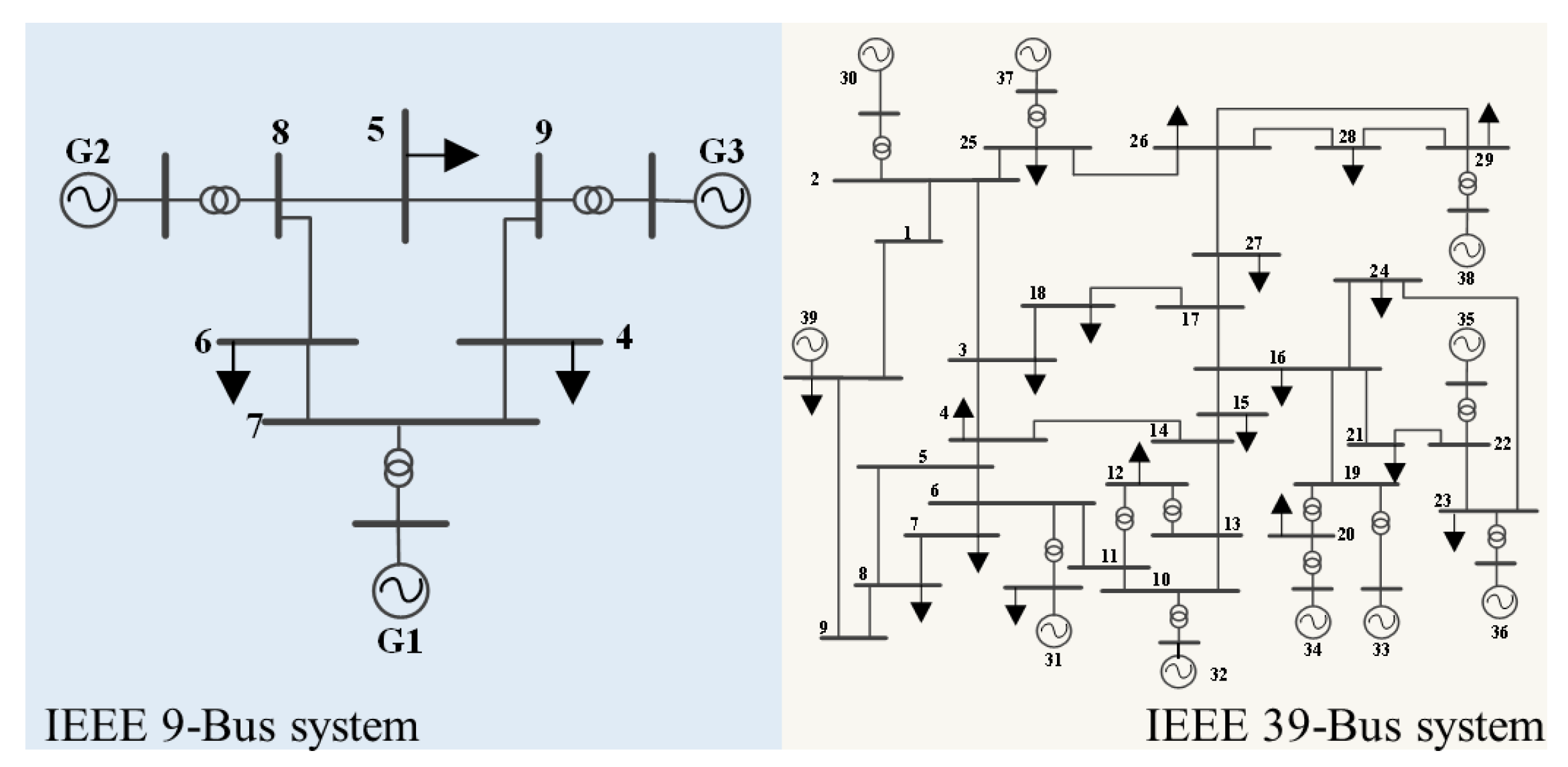
Based on the structural configurations of the IEEE 9-bus and 39-bus systems, the inertia levels of each node in the systems are evaluated by using the NFDC. The simulation model of the systems is shown in Figure 3. The IEEE 9-bus system contains 3 generators, 3 loads, and 9 branches, while the IEEE 39-bus system contains 10 generators, 21 loads, and 46 branches.

Based on the simulation models of the IEEE 9-bus system and 39-bus system, the inertia level of each node in the systems can be evaluated by the value of the NFDC. The parameters of the generators in the system, including the inertia coefficient, are shown in

Table 1. Generator parameters in IEEE 9-bus system and IEEE 39-bus system.

System	Unit Number	Generator Type	Nominal Capacity/MVA	Inertia Constant/s
IEEE9	G1	SG	200	20
	G2	SG	200	12
	G3	SG	100	6
IEEE39	G30	SG	400	4
	G31	SG	700	10
	G32	WF	800	10
	G33	WF	800	5
	G34	WF	700	5
	G35	SG	800	20
	G36	SG	700	20
	G37	SG	700	4
	G38	SG	1000	15
	G39	SG	1200	4

. WF indicates that the generator type of the unit is a wind farm.

Based on the NFDC, the inertia support capability of various nodes and the distribution of inertia resources in the power system can be effectively represented.

Table 2. The NFDC values for the IEEE 9-bus system.

Node Number	G1	G2	G3
R4	0.0252–0.0036i	0.0109–0.001i	0.0542–0.0043i
R5	0.0067–0.0004i	0.0358–0.0037i	0.065–0.0062i
R6	0.0251–0.0043i	0.0242–0.0023i	0.0237–0.0019i
R7	0.036–0.0031i	0.0102–0.0004i	0.0218–0.0001i
R8	0.007–0.0003i	0.0532–0.0036i	0.0294–0.0013i
R9	0.0066–0.0001i	0.0129–0.0006i	0.1172–0.007i

shows the values of the NFDC at each node in the IEEE 9-bus system.

G represents the generation nodes in the system and R refers to the network or load nodes. According to the evaluation results, the NFDC is a complex number, with the real part being much larger than the imaginary part. This is because the active power loss in the power system is primarily reflected in the branch impedance, which manifests as a larger real part in the NFDC. Therefore, when conducting index evaluations subsequently, the real part of the NFDC will be used as the basis for evaluating the inertia levels of the nodes.

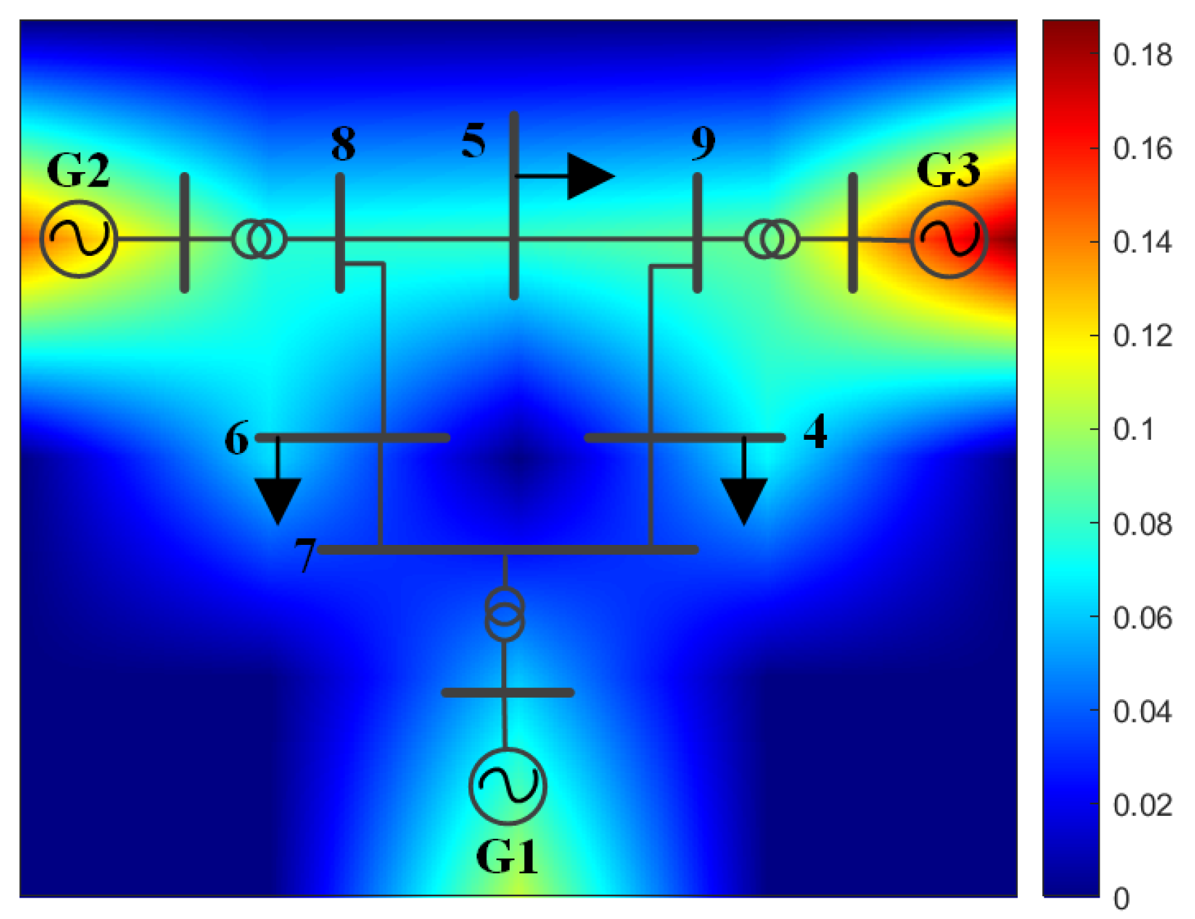
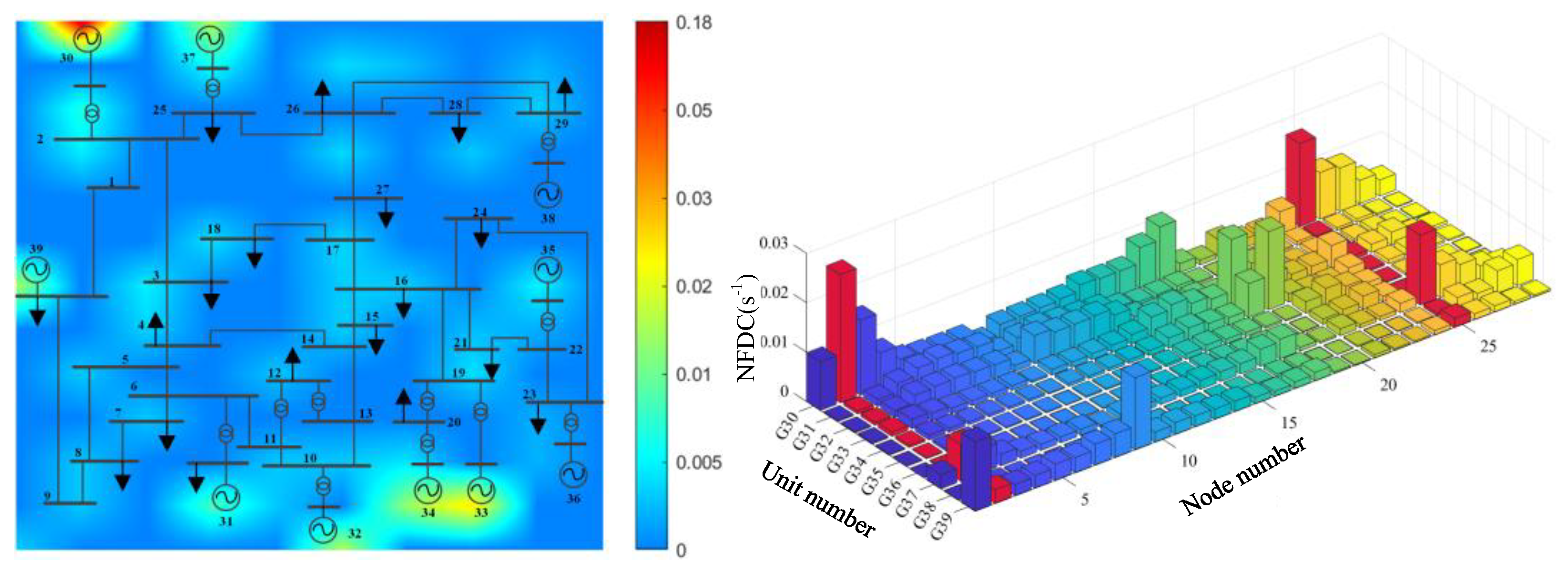
As shown in Figure 4, the inertia levels of each node in IEEE 9-bus system are presented in the form of a heat map. This approach allows for a more intuitive understanding of the inertia distribution characteristics of the system.

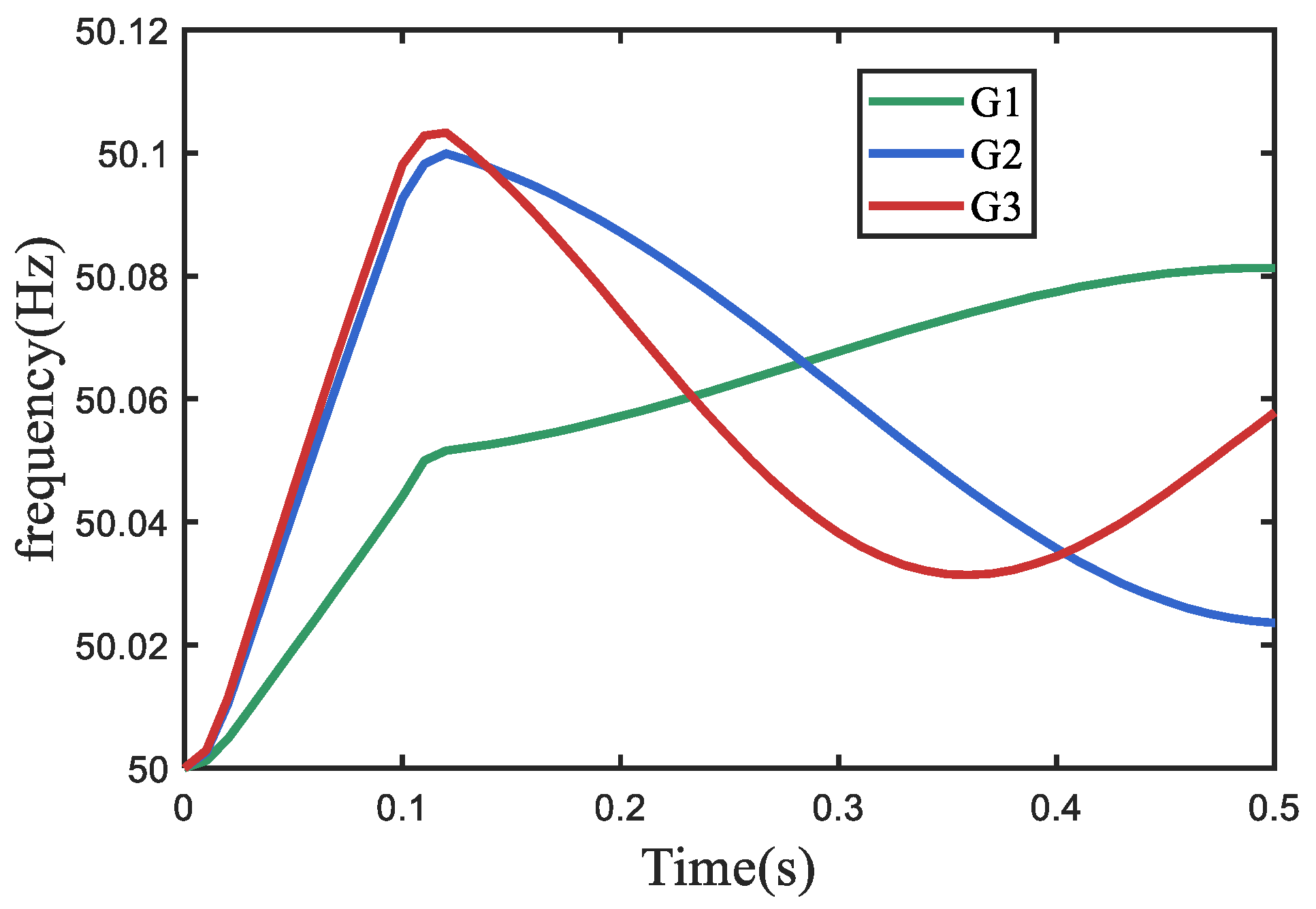
The power disturbance in the system is simulated by setting a single-phase short-circuit fault at bus R6 in IEEE 9-bus system. The frequency dynamic characteristics of three generators in IEEE 9-bus system can be observed through time-domain simulation. The simulation results are shown in Figure 5. It can be observed that during the occurrence of a power disturbance event, the frequency variation of G3 is the most pronounced, whereas that of G1 is the least significant. This is consistent with the situation represented by the NFDC, indicating that the NFDC can accurately reflect the inertia level of the nodes in the power system.

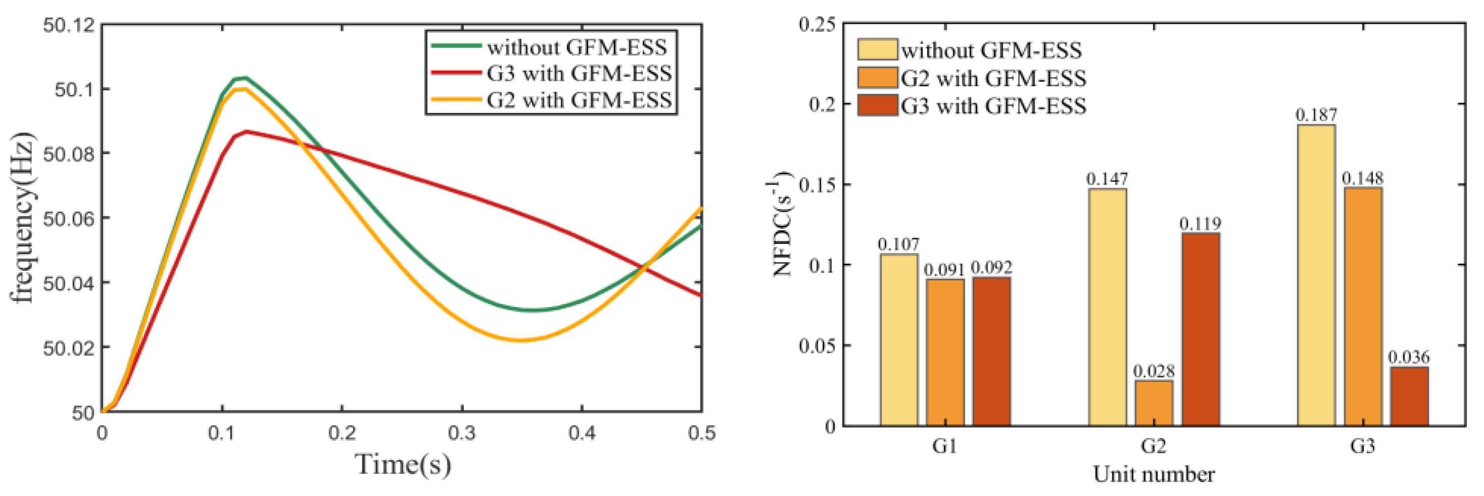
To observe the frequency characteristics of the three generators and the value of the NFDC, the GFM-ESS which has a nominal capacity of 30MW is implemented in the IEEE 9-bus system. The comparative results are shown in Figure 6.

According to the simulation results, after configuring the GFM-ESS, the RoCoF of each generator decreases, with the most significant decrease observed at the unit where the GFM-ESS is installed. The decrease in RoCoF is also reflected in the change in the NFDC value, indicating a positive correlation between the NFDC and RoCoF.

Based on the same method, the inertia distribution characteristics of the IEEE 39-bus system were evaluated. The NFDC evaluation results are shown in Figure 7.

According to the evaluation results, G30 belongs to the weak link in terms of the system inertia level, and G33 and G34 also have the risk of losing stability. When configuring the ESS, these locations can be given priority consideration.

4.2. Optimization Results Analysis

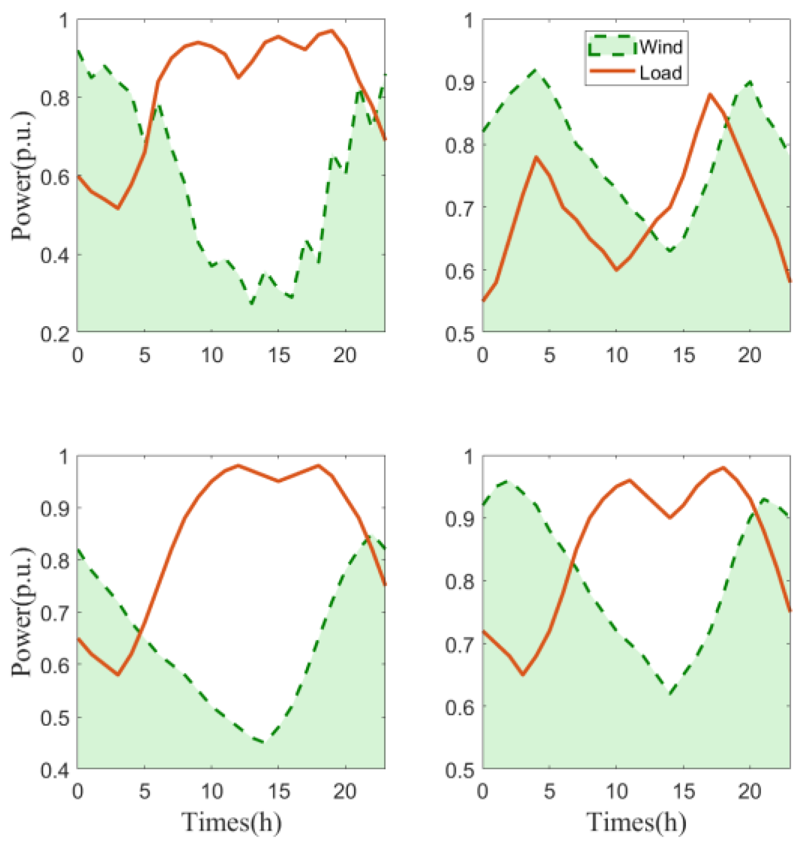
RESs and loads have different power curves in different seasons. In order to explore the inertia distribution characteristics of a power system during different time periods, this study considers four normalized power scenarios of wind and load, as shown in Figure 8, aiming to configure the GFM-ESS and GFL-ESS in the most economical way. This will help improve the utilization efficiency of RESs in the power system and enhance the inertia distribution characteristics of the power system.

G32 to G34 in the 39-bus system are designated as wind power. The predicted power output of the wind power and the power consumption of the load nodes are constrained in accordance with the power curves depicted in Figure 8.

The four typical power scenarios in Figure 8 include the power characteristics of summer, winter, and transitional seasons. In winter, the wind power output is generally higher throughout the day, while in summer, it is relatively lower. In transitional seasons, wind power exhibits higher levels in the early morning and evening, with lower output during midday. Regarding load characteristics, winter shows higher power consumption in the early morning and evening, while the peak load consumption in summer occurs around midday.

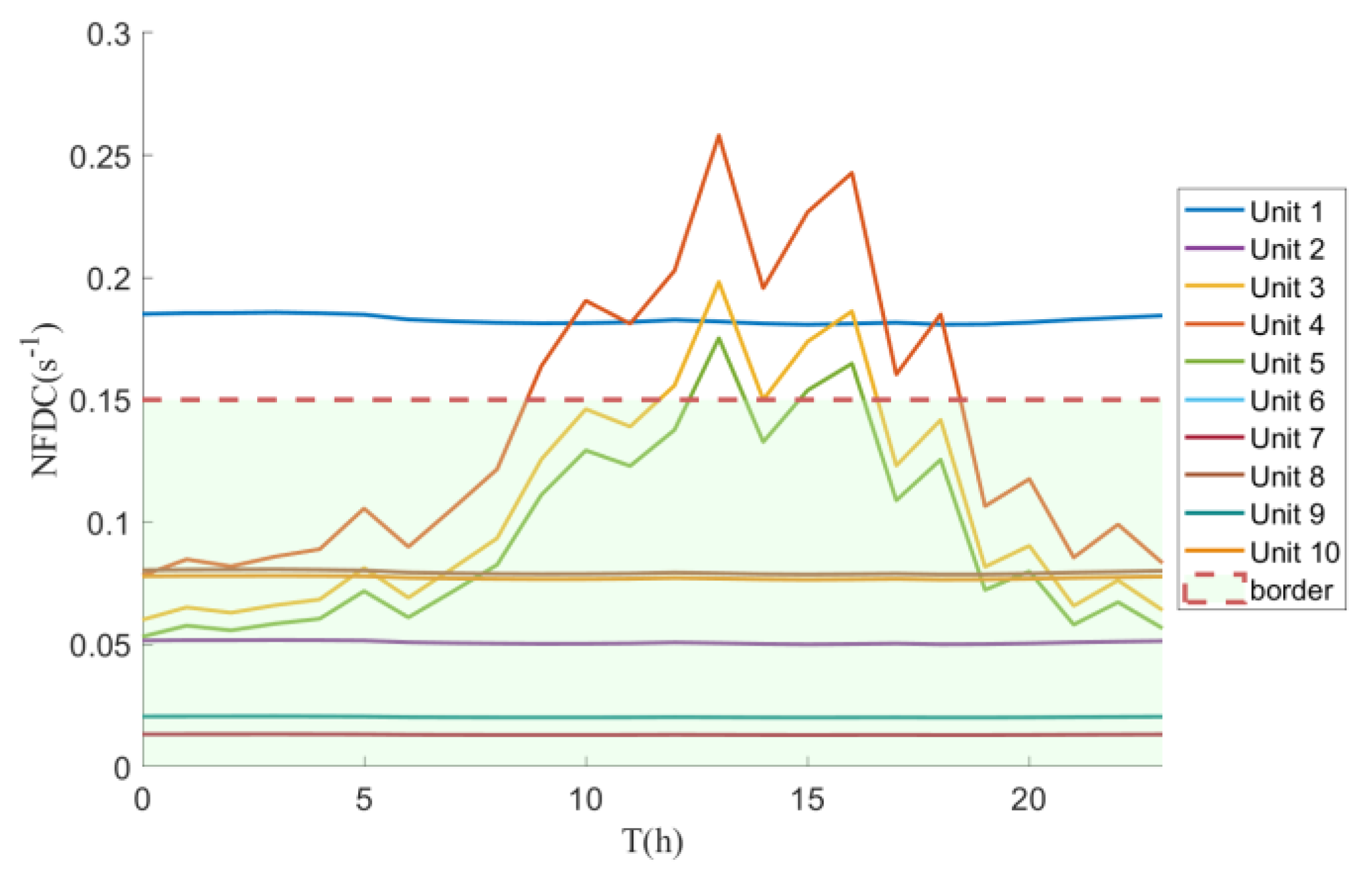
The value of the NFDC can represent the strength of the inertia support capability of each node in the power system. The variation in the NFDC of each generator in scenario 1 is shown in Figure 9.

Based on the simulation results, it can be observed that as the active power output changes, the inertia level of wind power will change significantly. At the same time, the inertia support capability of SGs is hardly affected by their active power output. This is because the inertia response characteristics of SGs primarily rely on their rotational inertia. In contrast, wind power is limited by its control strategy and the characteristics of power electronic devices, which makes it difficult for its active power to be fully released.

The relevant parameters of the generator and ESS are presented in

Table 3. Related parameters of SG.

	am/(¥·MW−2)	bm/(¥·MW−1)	cm/(¥)	${\mathit{c}}_{\mathit{i},\mathbf{res}}^{\mathbf{re}}$/(¥·W−1)
SG	0.03	97.65	1229.69	100

and

Table 4. Related parameters of ESS.

	${\mathit{k}}_{\mathbf{GFL}}^{\mathbf{P}}$/(¥·MW−1)	${\mathit{k}}_{\mathbf{GFM}}^{\mathbf{p}}$/(¥·MW−1)	r/%	EIC/(s·MW−1)	L/Year
ESS	250	300	6	0.2	3

, including the power generation cost coefficient, RES penalty coefficient, and cost coefficient of the ESS. By outputting active power, the GFM-ESS can provide inertia support capability, which is represented by the equivalent inertia constant (EIC).

The optimization configuration results of ESS, calculated under various scenarios, are presented in

Table 5. The configuration locations and operation costs of ESSs under various scenarios.

Typical Scenarios	The Operation Cost of SGs (Million ¥)	The Configuration Cost of ESSs (Million ¥)	The Configuration Location	The Allocated Capacity of GFL-ESSs (MW)	The Allocated Capacity of GFM-ESSs (MW)
Scenario 1	486.74	6.389	G30	127.182	68.548
			G32	89.527	71.363
			G33	222.899	63.031
Scenario 2	378.33	1.486	G30	0	68.548
			G33	62.19	14.801
Scenario 3	586.9	5.896	G30	230.492	68.548
			G32	169.36	0
			G33	115.476	27.334
Scenario 4	581.6	1.99	G30	30.952	68.548
			G33	82.698	16.802

. The system inertia demand, the installation locations of the ESSs, and the operating costs of the generators are solved based on the CPLEX solver (version 12.10.0.0). The optimization model aims to minimize the total system operating cost while ensuring that the inertia levels at each node meet the standards, and solves for the configuration, location, capacity, and type of ESS.

The capacity demand of the GFM-ESS is quantified according to the value of the NFDC, and the total configured capacity of ESSs can be calculated based on the optimization configuration method. When the total configuration capacity of ESSs is less than the required capacity of the GFM-ESS, all available resources of the ESSs will be prioritized for the construction of the GFM-ESS. Since the configuration cost of the GFM-ESS is relatively high, the GFL-ESS will be additionally configured when the total configured capacity of the ESSs is larger than the capacity requirement of the GFM-ESS. As a result, the power system can not only ensure its own stable operation but can also save the configuration cost of the ESS.

Based on the NFDC, it is known that the inertia level of G30 is relatively low, for which the GFM-ESS should be configured. G32 and G33 belong to wind power, and the configuration of the GFM-ESS is influenced by the power output of the wind power.

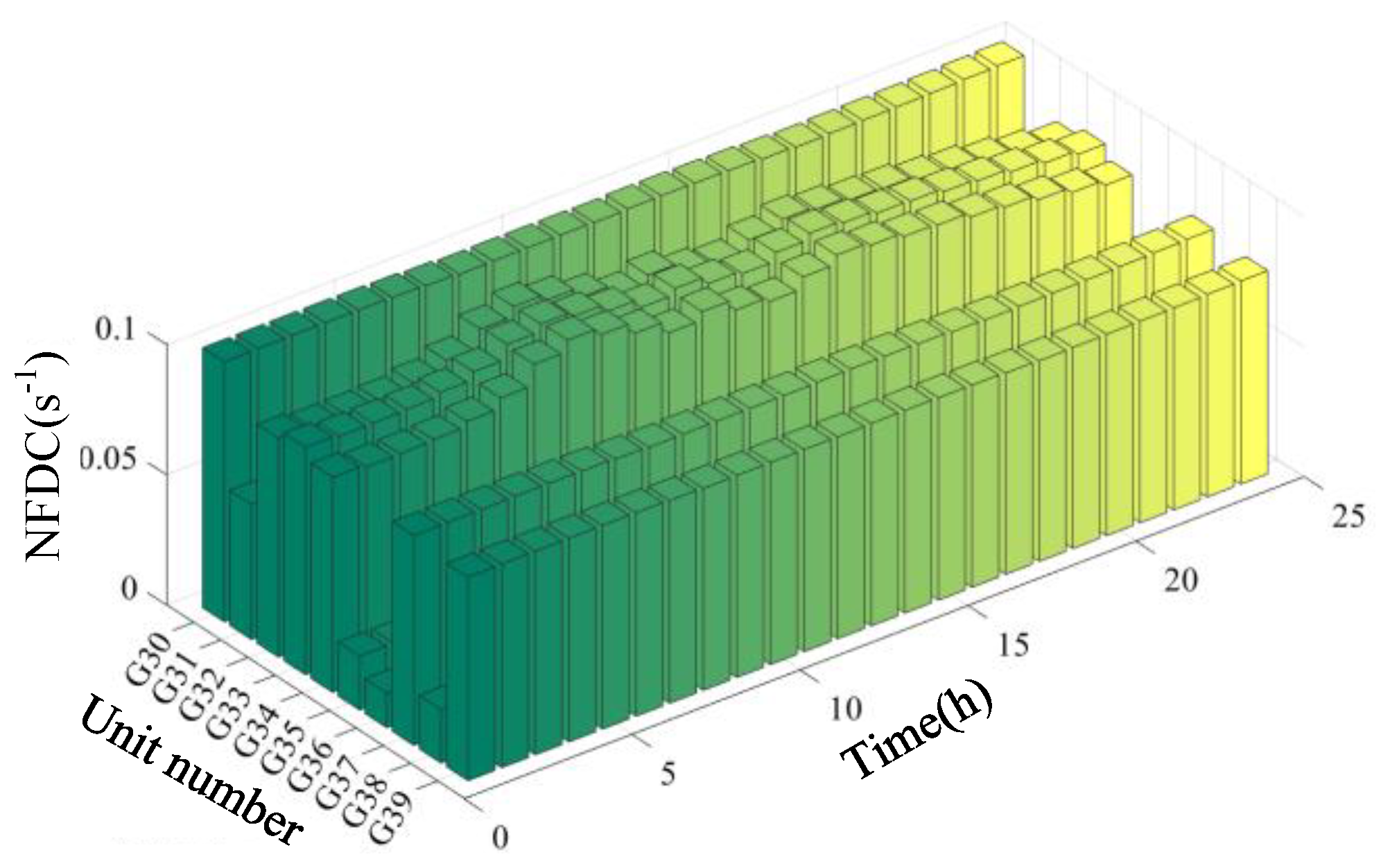
Before configuring the ESS, the inertia levels of various nodes in the system are relatively low. As shown in the system inertia distribution in Figure 8, the G30 node exhibits the weakest inertia support capability, where its value of NFDC is 0.18. As shown in Figure 9, with changes in the active power output of RESs, the value of the NFDC at certain generators may increase to around 0.25. This will weaken the inertia support capability of RESs, making the power system more prone to instability risks. Based on the energy storage allocation scheme of Scenario 1, a GFM-ESS can be constructed, and the variation in the NFDC as shown in Figure 10 can be described.

After the ESS is configured, the NFDC of all generators in 39-bus system is less than 0.1. At the same time, the inertia distribution characteristics of the power system have also been enhanced. Moreover, the distribution of the inertia resources of the power system has become more balanced.

In summary, this section first validates the feasibility of the value of the NFDC in assessing the inertia distribution of the power system. Subsequently, an optimization configuration method for the GFL-ESS and GFM-ESS is devised by integrating typical wind-load operation scenarios. Finally, the effectiveness of the proposed configuration method is verified through the improved IEEE 39-bus system. These findings can be used by stakeholders and policy makers to promote the full exploitation of the GFM-ESS in renewable energy power systems.

5. Discussions

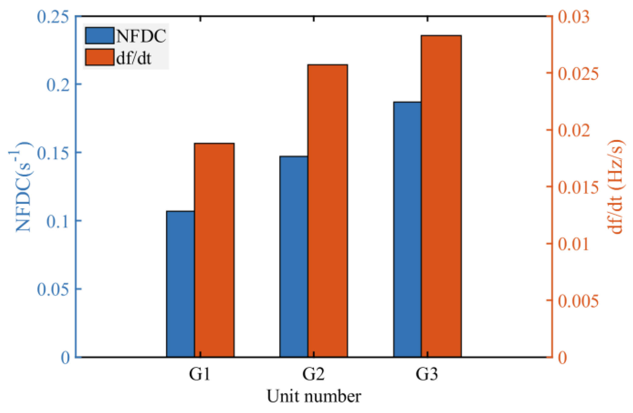
The RoCoF of three generators in the IEEE 9-bus system was detected using the NFDC evaluation method and the power system inertia estimation method proposed in [26], respectively. A single-phase short-circuit fault was simulated at bus R6 as the power disturbance event. The RoCoF of the generator in [28] was expressed by Equation (28). The comparative evaluation results of the two methods are presented in Figure 11.

$${\displaystyle \frac{\mathrm{d}{f}_i}{\mathrm{d}t}}={\displaystyle \frac{-\Delta P_i}{2H_{Sbase}}}{f}_0$$

(28)

The simulation results indicate that the inertia estimation method proposed in [26] and the method presented in this paper yield consistent results. In the IEEE 9-bus system, the inertia support capacity of G3 is relatively weak.

Compared to the traditional estimation method, the method proposed in this paper does not require the active power variation at each node to assess the inertia levels of weak nodes, making it highly valuable for power system planning. However, for extreme fault scenarios, such as when a particular node in the system faces a high risk of failure, it is more appropriate to evaluate the most severe fault scenario at that node using the method in [26]. The inertia distribution characteristics can be more accurately determined by calculating the time-domain results. Moreover, the derivation of the NFDC is primarily based on the power system network equations and the inertia coefficients of generators. Compared to the method in [26], its physical meaning is less clear, and the value of the NFDC can only be applied in the fields of power system planning and stability assessment.

6. Conclusions

With the continuous integration of RESs, critical challenges like varying inertia distribution characteristics and the decline of the inertia support capability of power systems have become increasingly prominent. This study focuses on analyzing the impact of generator sets on the inertia distribution characteristics in a power system. Moreover, based on the grid structure of the power system, the NFDC is proposed to evaluate the frequency dynamic characteristics of each node. This proposed evaluation method can quantify the configuration requirements of a GFM-ESS. Aiming at the inertia distribution characteristics of power system, an optimization configuration method for both a GFL-ESS and GFM-ESS is proposed. The conclusions drawn in this study are as follows:

The evaluation method based on the NFDC can describe the inertia distribution characteristics of a power system, which are determined by the distribution of generators and ESSs. The value of the NFDC is subject to the influence of multiple factors, including the inertia time constant of generators, the power output of RESs, and the grid structure of the power system. The elevated value of the NFDC at a certain bus signifies the degraded inertia response in the power system.

The NFDC can be utilized to formulate the operational boundaries of the power system and clarify the requirement of inertia resources in the power system. By means of rational configuration of GFM-ESSs and GFL-ESSs, the inertia resource in a GFM-ESS can be fully harnessed, thereby enabling the ESS to exert its regulatory ability in stabilizing power fluctuations. However, compared to traditional methods, the physical meaning of the NFDC is less clear, and its applicability in extreme scenarios is relatively weaker.

A GFM-ESS can effectively enhance the accommodation level of RESs and provide inertia support capability. The operational cost of the system and the configuration cost of ESSs can be reduced by employing the optimization configuration method proposed in this study. This method can also clarify the configuration requirements for both GFL-ESSs and GFM-ESSs. Furthermore, the upper and lower limits of the NFDC can be more clearly defined based on the operational standards of renewable energy power systems. Additionally, by incorporating certain extreme operating scenarios and using time-domain analysis methods, the weak nodes of the power system can be fully identified, enabling more reliable planning and configuration of ESSs.

References

1. Milano, F.; Dörfler, F.; Hug, G.; Hill, D.J.; Verbič, G. Foundations and Challenges of Low-Inertia Systems (Invited Paper). In Proceedings of the 2018 Power Systems Computation Conference, Dublin, Ireland, 11–15 June 2018. [Google Scholar]
2. Kroposki, B.; Johnson, B.; Zhang, Y.; Gevorgian, V.; Denholm, P.; Hodge, B.-M.; Hannegan, B. Achieving a 100% Renewable Grid: Operating Electric Power Systems with Extremely High Levels of Variable Renewable Energy. IEEE Power Energy Mag. 2017, 15, 61–73. [Google Scholar] [CrossRef]
3. Homan, S.; Mac Dowell, N.; Brown, S. Grid frequency volatility in future low inertia scenarios: Challenges and mitigation options. Appl. Energy 2021, 290, 116723. [Google Scholar] [CrossRef]
4. Peng, Z.; Peng, Q.; Zhang, Y.; Han, H.; Yin, Y.; Liu, T. Online Inertia Allocation for Grid-Connected Renewable Energy Systems Based on Generic ASF Model Under Frequency Nadir Constraint. IEEE Trans. Power Syst. 2024, 39, 1615–1627. [Google Scholar] [CrossRef]
5. Zhang, Z.; Du, E.; Teng, F.; Zhang, N.; Kang, C. Modeling Frequency Dynamics in Unit Commitment with a High Share of Renewable Energy. IEEE Trans. Power Syst. 2020, 35, 4383–4395. [Google Scholar] [CrossRef]
6. Ma, N.; Wang, D. Extracting Spatial-Temporal Characteristics of Frequency Dynamic in Large-Scale Power Grids. IEEE Trans. Power Syst. 2019, 34, 2654–2662. [Google Scholar] [CrossRef]
7. Liu, J.; Wang, C.; Bi, T. Node equivalent inertia index for temporal-spatial frequency dynamics of renewable energy power system and its applications. Proc. CSEE 2023, 43, 7773–7789. [Google Scholar]
8. Li, Z.; Yang, L.; Xu, Y. A dynamics-constrained method for distributed frequency regulation in low-inertia power systems. Appl. Energy 2023, 344, 121256. [Google Scholar] [CrossRef]
9. Sang, L.; Xu, Y.; Long, H.; Hu, Q.; Sun, H. Electricity Price Prediction for Energy Storage System Arbitrage: A Decision-Focused Approach. IEEE Trans. Smart Grid 2022, 13, 2822–2832. [Google Scholar] [CrossRef]
10. Du, W.; Tuffner, F.K.; Schneider, K.P.; Lasseter, R.H.; Xie, J.; Chen, Z.; Bhattarai, B. Modeling of Grid-Forming and Grid-Following Inverters for Dynamic Simulation of Large-Scale Distribution Systems. IEEE Trans. Power Deliv. 2021, 36, 2035–2045. [Google Scholar] [CrossRef]
11. Denis, G.; Prevost, T.; Debry, M.; Xavier, F.; Guillaud, X.; Menze, A. The migrate project: The challenges of operating a transmission grid with only inverter-based generation. A grid-forming control improvement with transient current-limiting control. IET Renew. Power Gener. 2018, 12, 523–529. [Google Scholar] [CrossRef]
12. Lasseter, R.; Chen, Z.; Pattabiraman, D. Grid-Forming Inverters: A Critical Asset for the Power Grid. IEEE J. Emerg. Sel. Top. Power Electron. 2020, 8, 925–935. [Google Scholar] [CrossRef]
13. Sun, M.; Liu, G.; Popov, M.; Terzija, V.; Azizi, S. Underfrequency Load Shedding Using Locally Estimated RoCoF of the Center of Inertia. IEEE Trans. Power Syst. 2021, 36, 4212–4222. [Google Scholar] [CrossRef]
14. Tuttelberg, K.; Kilter, J.; Wilson, D.; Uhlen, K. Estimation of Power System Inertia from Ambient Wide Area Measurements. IEEE Trans. Power Syst. 2018, 33, 7249–7257. [Google Scholar] [CrossRef]
15. Pulgar-Painemal, H.; Wang, Y.J.; Silva-Saravia, H. On Inertia Distribution, Inter-Area Oscillations and Location of Electronically-Interfaced Resources. IEEE Trans. Power Syst. 2018, 33, 995–1003. [Google Scholar] [CrossRef]
16. Gayathri, K.; Jenas, M.K. A Practical Approach to Inertia Distribution Monitoring and Impact of Inertia Distribution on Oscillation Baselining Study for Renewable Penetrated Power Grid. IEEE Syst. J. 2023, 17, 3593–3601. [Google Scholar]
17. You, S.T.; Liu, Y.; Kou, G.F.; Zhang, X.M.; Yao, W.X.; Su, Y.; Hadley, S.W.; Liu, Y.L. Non-Invasive Identification of Inertia Distribution Change in High Renewable Systems Using Distribution Level PMU. IEEE Trans. Power Syst. 2018, 33, 1110–1112. [Google Scholar] [CrossRef]
18. Mallemaci, V.; Mandrile, F.; Carpaneto, E.; Bojoi, R. Simplified Virtual Synchronous Compensator with Grid–Forming Capability. IEEE Trans. Ind. Appl. 2023, 59, 6203–6219. [Google Scholar] [CrossRef]
19. Swain, N.; Sinha, N.; Behera, S. Stabilized Frequency Response of a Microgrid Using a Two-Degree-of-Freedom Controller with African Vultures Optimization Algorithm. ISA Trans. 2023, 140, 412–425. [Google Scholar] [CrossRef]
20. Fotis, G.; Sijakovic, N.; Zarkovic, M.; Ristic, V.; Terzic, A.; Vita, V.; Zafeiropoulou, M.; Zoulias, E.; Maris, T.I. Forecasting Wind and Solar Energy Production in the Greek Power System Using ANN Models. WSEAS Trans. Power Syst. 2023, 18, 373–391. [Google Scholar] [CrossRef]
21. Rahimi, T.; Ding, L.; Kheshti, M.; Faraji, R.; Guerrero, J.M.; Tinajero, G.D.A. Inertia Response Coordination Strategy of Wind Generators and Hybrid Energy Storage and Operation Cost-Based Multi-Objective Optimizing of Frequency Control Parameters. IEEE Access 2021, 9, 74684–74702. [Google Scholar] [CrossRef]
22. Wu, C.; Liu, C.; Huang, W.; Zeng, P.; Yuan, H.; Xin, H. Method for Selecting and Sizing Grid Type Converters to Improve the Stability of New Energy Power Systems. Autom. Electr. Power Syst. 2023, 47, 130–136. [Google Scholar]
23. Yang, T.; Huang, Y.; He, Z.; Wang, D.; Tang, J.R.; Xie, C. Optimized Configuration of Fixed-Capacity and Location Selection for Grid-Forming Energy Storage Power Station Based on Multi-Timescale Regulation. Autom. Electr. Power Syst. 2024, 48, 54–64. [Google Scholar]
24. Fotis, G.; Vita, V.; Maris, T.I. Risks in the European Transmission System and a Novel Restoration Strategy for a Power System after a Major Blackout. Appl. Sci. 2022, 13, 83. [Google Scholar] [CrossRef]
25. Ebrahimi, M.; Khajehoddin, S.A.; Karimi-Ghartemani, M. An Improved Damping Method for Virtual Synchronous Machines. IEEE Trans. Sustain. Energy 2019, 10, 1491–1500. [Google Scholar] [CrossRef]
26. Yi, Z.; Xu, Y.; Wang, H.; Sang, L. Coordinated Operation Strategy for a Virtual Power Plant with Multiple DER Aggregators. IEEE Trans. Sustain. Energy 2021, 12, 2445–2458. [Google Scholar] [CrossRef]
27. Yuan, H.; Li, F.; Wei, Y.; Zhu, J. Novel Linearized Power Flow and Linearized OPF Models for Active Distribution Networks with Application in Distribution LMP. IEEE Trans. Smart Grid 2018, 9, 438–448. [Google Scholar] [CrossRef]
28. Ashton, P.M.; Saunders, C.S.; Taylor, G.A.; Carter, A.M.; Bradley, M.E. Inertia Estimation of the GB Power System Using Synchrophasor Measurements. IEEE Trans. Power Syst. 2015, 30, 701–709. [Google Scholar] [CrossRef]
Figure 1. The topology and control diagram of the GFM-ESS unit.
Applsci 15 05544 g001
Figure 2. The power control loop of the grid-forming energy storage system.
Applsci 15 05544 g002
Figure 3. Simulation models of IEEE 9-bus system and IEEE 39-bus system.
Applsci 15 05544 g003
Figure 4. The inertia distribution characteristics of the IEEE 9-bus system.
Applsci 15 05544 g004
Figure 5. The frequency dynamic characteristics of the three generators in the IEEE 9-bus system.
Applsci 15 05544 g005
Figure 6. The frequency characteristics and NFDC of G3 after configuring the GFM-ESS.
Applsci 15 05544 g006
Figure 7. The inertia distribution characteristics of the IEEE 39-bus system.
Applsci 15 05544 g007
Figure 8. Typical normalized power scenarios of wind and load.
Applsci 15 05544 g008
Figure 9. The variation in the NFDC of generators in typical scenarios.
Applsci 15 05544 g009
Figure 10. The variation in the NFDC of generators after the configuration of ESS.
Applsci 15 05544 g010
Figure 11. Comparative evaluation results of inertia level in IEEE 9-Bus System.
Applsci 15 05544 g011