Real-Time Object Detection and Distance Measurement Enhanced with Semantic 3D Depth Sensing Using Camera–LiDAR Fusion

Abstract

Camera and LiDAR data fusion has been a popular research area, especially in the field of autonomous vehicles. This study evaluates the efficiency and accuracy of different depth point extraction methods, including Point-by-Point (PbyP), Complete Region Depth Extraction (CoRDE), Central Region Depth Extraction (CeRDE), and Grid Central Region Depth Extraction (GCRDE), across object categories such as person, bicycle, car, bus, and truck, and occlusion levels ranging from 0 to 3. The approaches are assessed based on extraction time, accuracy, and root mean squared error (RMSE). Bounding box-based methods, such as PbyP and CoRDE, consistently show slower extraction times compared to segmentation mask methods, with CeRDE being the most efficient in terms of computational speed. However, segmentation mask methods, particularly CeRDE and GCRDE, offer superior accuracy, especially for complex objects like trucks and cars, where bounding box methods struggle, particularly at higher occlusion levels. In terms of RMSE, segmentation mask methods consistently outperform bounding box methods, providing more precise depth estimations, particularly for larger and more occluded objects. Overall, segmentation mask methods are preferred for applications where accuracy is critical, despite their slower processing speed, while bounding box methods are suitable for real-time applications requiring faster depth extraction. GeRDE offers a balance between speed and accuracy, making it ideal for tasks needing both efficiency and precision.

1. Introduction

In recent years, the demand for accurate and robust perception systems in autonomous vehicles, robotics, and other computer vision applications has led to the development of multi-sensor fusion techniques. Combining data from various sensors, such as Light Detection and Ranging (LiDAR) devices and cameras, enables more comprehensive and reliable scene understanding. Cameras provide high-resolution color images that capture texture and appearance, while LiDAR generates three-dimensional (3D) point clouds that offer precise spatial information, including distance measurements and object shapes. Each sensor has its strengths and weaknesses: cameras are affected by lighting conditions, and LiDAR lacks rich appearance information but excels at measuring distances accurately. Thus, fusing data from both types of sensors can significantly improve the performance of perception systems, especially for tasks like object detection and distance estimation.

Traditionally, LiDAR-camera fusion involves projecting LiDAR point cloud data onto the camera image plane using extrinsic and intrinsic calibration parameters, where the LiDAR points within the camera’s field of view are used to enhance perception tasks. This fusion typically includes combining spatial information (i.e., the 3D positions) from LiDAR with appearance features from camera images, followed by applying object detection algorithms to locate and classify objects. After detecting objects, the challenge lies in associating LiDAR points with object bounding boxes to determine their precise distances.

This research proposes three novel approaches for extracting object distances using camera-LiDAR sensor fusion: Complete Region Depth Extraction (CoRDE), Central Region Depth Extraction (CeRDE), and Grid Central Region Depth Extraction (GCRDE). Each method focuses on improving distance estimation accuracy by leveraging sparse depth maps generated from LiDAR data and refining object-specific distance calculations using object detection results. By comparing the three methods, this study aims to highlight the strengths and limitations of each approach, providing insights into more accurate and efficient distance estimation for real-time applications such as autonomous driving.

1.1. Research Questions and Motivation

This study aims to investigate object distance estimation using camera-LiDAR sensor fusion under varying levels of occlusion. While previous methods primarily focus on fully visible objects using raw point cloud data, our approach considers easy, moderate, and hard occlusion scenarios and uses a projected transparent sparse depth map to speed up the process. Based on this motivation, we address the following research questions.

• How can object distance be accurately estimated from fused camera-LiDAR data in the presence of different occlusion levels?
• How do the bounding box and the segmentation-based depth extraction methods perform under easy, moderate, and hard occlusion conditions?
• Can the transparent sparse depth map projected from LiDAR data provide sufficient information for reliable object distance estimation despite the lack of intermediate depth data?

1.2. List of Main Contributions

The following is a list of the main contributions that this work makes:

• We propose a camera-LiDAR fusion pipeline that generates transparent Sparse Depth Images and normalizes depth values for accurate spatial mapping.
• We introduce three novel object depth extraction methods. Complete Region Depth Extraction (CoRDE), Central Region Depth Extraction (CeRDE), and Grid Central Region Depth Extraction (GCRDE).
• We fuse YOLOv8 object detection with LiDAR clustering to improve depth estimates for object regions.
• We evaluate our methodologies on objects in the KITTI dataset with different occlusion levels, evaluating mean time and point, accuracy, and root mean square error (RMSE), through a truth table.
• Our findings show the advantages of segmentation masks compared to bounding boxes in object distance estimation and establish CeRDE as a method that effectively balances precision and speed.

1.3. Brief Description of the Following Paper Sections

The subsequent sections of the article are structured as follows. Section 2 examines related work on camera-LiDAR fusion and object distance estimation. Section 3 defines our suggested methodology, which encompasses the generation of transparent depth image generation, YOLOv8 detection, and three depth point extracting strategies for estimating distance. Section 4 shows the evaluation procedure, which involves the description of the dataset, the generation of the ground truth table, and analysis formulas. Section 5 delineates the implementation results and comparative evaluations. Section 6 ultimately concludes this study and defines further research.

2. Related Works

Multi-sensor fusion has been a popular research area, especially in the field of autonomous vehicles, where accurate environmental perception is critical. Combining LiDAR and camera data has been shown to improve object detection, tracking, and distance estimation compared to using a single sensor. Several existing approaches aim to fuse LiDAR and camera data at different levels, including early fusion, late fusion, and deep fusion techniques.

In early fusion, sensor data are combined at an early stage of processing, allowing the perception system to utilize raw data from multiple sensors. One common approach is to project LiDAR points onto the camera image plane, aligning the data in 2D space using calibration parameters. Geiger et al. employed this technique for depth estimation in urban environments [1]. Charles et al. proposed an early fusion technique where RGB images and depth information from LiDAR are fused to enhance object detection [2]. The fused data are then passed through a neural network for classification. However, early fusion methods may struggle to handle differences in sensor resolution and noise from each modality, limiting their effectiveness in certain scenarios.

Late fusion involves fusing the sensor data after independent feature extraction from each modality. Ku et al. introduced a 3D object detection system where features from LiDAR point clouds and camera images are extracted separately using convolutional neural networks (CNNs) before being combined for final object detection [3]. Late fusion methods offer flexibility in handling sensor-specific noise and characteristics, but may miss potential correlations between raw sensor data.

Deep learning methods for sensor fusion have become increasingly prominent due to their ability to learn very complicated feature representations. Chen et al. introduced Multi-View 3D (MV3D), a framework that processes LiDAR point clouds and RGB images to generate 3D object proposals and performs detection in a joint 2D-3D space [4]. Similarly, the PointPainting method paints LiDAR point clouds with semantic information from image segmentation, enabling the network to leverage both 2D and 3D data for improved detection [5]. However, deep fusion techniques frequently require large amounts of annotated data and considerable processing resources, making them challenging for real-time applications.

In distance estimation, multiple strategies have been explored to accurately determine object distances using LiDAR and camera fusion. Nabati et al. demonstrated a camera-radar sensor fusion architecture for precise object detection and the estimation of distance in autonomous driving contexts [6]. Their approach utilizes radar view and RGB images, employing a middle-fusion technique to combine these data sources effectively [6]. Similarly, a study by Favelli et al. proposed an accurate data fusion technique between a stereolabs ZED2 camera and a LiDAR sensor to determine object distance, hence improving the vehicle’s perception capabilities [7].

Sparse depth maps derived from LiDAR data are increasingly used in fusion tasks to address the low spatial resolution of LiDAR sensors. Sparse-to-dense depth estimation methods have been explored, where sparse LiDAR points are used to estimate dense depth maps corresponding to the camera’s field of view. This technique allows for better handling of regions where LiDAR data may be sparse, such as at far distances or occluded areas. Work by Ma et al. demonstrated an efficient depth completion approach that combines sparse depth measurements from LiDAR with RGB images using a deep neural network, improving depth map quality [8]. Additionally, the Sparse LiDAR and Stereo Fusion (SLS-Fusion) method integrates data from LiDAR and stereo cameras through a neural network for depth estimation, resulting in enhanced dense depth maps and improving 3D object detection performance [9].

In addition to the above, transformer-based multi-modal fusion and attention-based camera-LiDAR fusion architectures have recently emerged as powerful tools for camera-LiDAR fusion. BAFusion [10] introduces a bidirectional attention fusion module for 3D object detection in autonomous driving. It uses cross-attention and a cross-focused linear attention fusion layer to improve performance, particularly for smaller objects. FusionViT [11] introduces a vision transformer-based 3D object detection model that outperforms existing methods and image-point clouds deep fusion approaches in real-world object detection benchmark datasets. Moreover, CLFT [12], LCPR [13], and CalibFormer [14] propose a network that is a view converter-based network for semantic segmentation, location identification, and automatic LiDAR camera calibration, respectively, enhancing multimodal place recognition and robustness to viewpoint changes in autonomous vehicles by combining LiDAR point clouds with multi-view RGB images.

Recent studies have introduced innovative methods to further enhance camera-LiDAR fusion for distance estimation and 3D object detection. Dong et al. proposed SuperFusion, a multilevel fusion network integrating LiDAR and camera data for the creation of long-range HD maps [15]. Similarly, Dam et al. introduced AYDIV, a framework that incorporates a tri-phase alignment method to improve long-distance detection [16]. AYDIV addresses challenges arising from data discrepancies between the sparse data of LiDAR and the high resolution of cameras, improving performance on datasets like Waymo Open Dataset and Argoverse2 [16]. Another notable contribution is that Kumar et al. proposed an approach for multi-sensor fusion, where LiDAR and camera data are integrated to enhance both object detection and distance estimation. Their method needs relatively clear object visibility, like fully visible or minimally occluded objects, to ensure accurate distance predictions [17]. In contrast, the methods proposed in our study are designed to operate effectively across varying levels of object visibility, including easy, medium, hard, and unknown cases. By utilizing the transparent sparse depth maps and object detection outputs, the proposed approaches aim to offer robust distance estimation even under partial occlusion or challenging perception conditions, addressing real-world scenarios where objects are not always fully observable.

Object detection plays a critical role in multi-sensor fusion systems, especially for tasks involving depth estimation from LiDAR and camera data. The YOLO (You Only Look Once) family of models has been widely adopted due to its high detection speed and competitive accuracy. Recent versions, including YOLOv7 [18], YOLOv8 [19], YOLOv9 [20], and YOLOv10 [21], support both bounding box detection and instance segmentation, making them suitable for tasks requiring detailed spatial information.

Earlier YOLO versions, such as YOLOv3 [22], YOLOv4 [23], YOLOv5 [24], and YOLOv6 [25], only support bounding box detection and do not provide native segmentation mask output. This limitation reduces their effectiveness for tasks that require pixel-level accuracy, such as extracting depth values from specific object regions in sparse depth maps through Camera-LiDAR fusion.

This study chose YOLOv8 due to its balance of performance, speed, and ease of integration. YOLOv8 is lightweight and optimized for real-time applications, which aligns with the goals of this work, where fast and reliable detection is necessary for accurate depth extraction from sparse LiDAR data. It is particularly useful for methods requiring precise object localization to extract depth values from segmented regions.

Building on the advancements in LiDAR-camera fusion, this research proposes three novel methods aimed at improving object distance estimation. These methods take advantage of the transparent sparse depth maps generated from LiDAR data, combined with object detection results from the camera, to refine distance estimates. The CoRDE calculates object distances by extracting all pixel values within the detected bounding box and averaging their distances. The CeRDE focuses on the central region of the object to mitigate errors caused by sparse LiDAR points, while the GCRDE subdivides the object region into smaller grids, performing depth extraction for each grid cell to achieve a more reliable overall distance estimate. These approaches aim to address challenges associated with sparse LiDAR data and noisy object detection results, offering a more accurate and efficient solution for distance estimation.

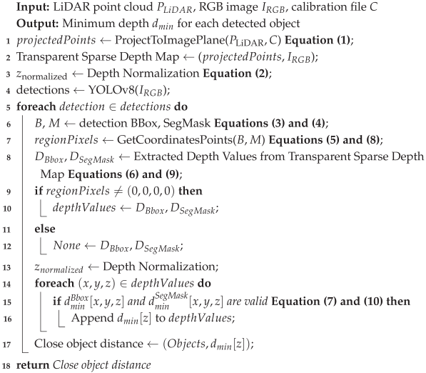
3. Methodology

This methodology outlines a novel approach for object detection and distance measurement that integrates camera and LiDAR data by converting point-cloud data into a 2D transparent Sparse Depth Image. A detailed description of each algorithm can be found in Appendix A.

3.1. LiDAR-Camera Processing Pipeline

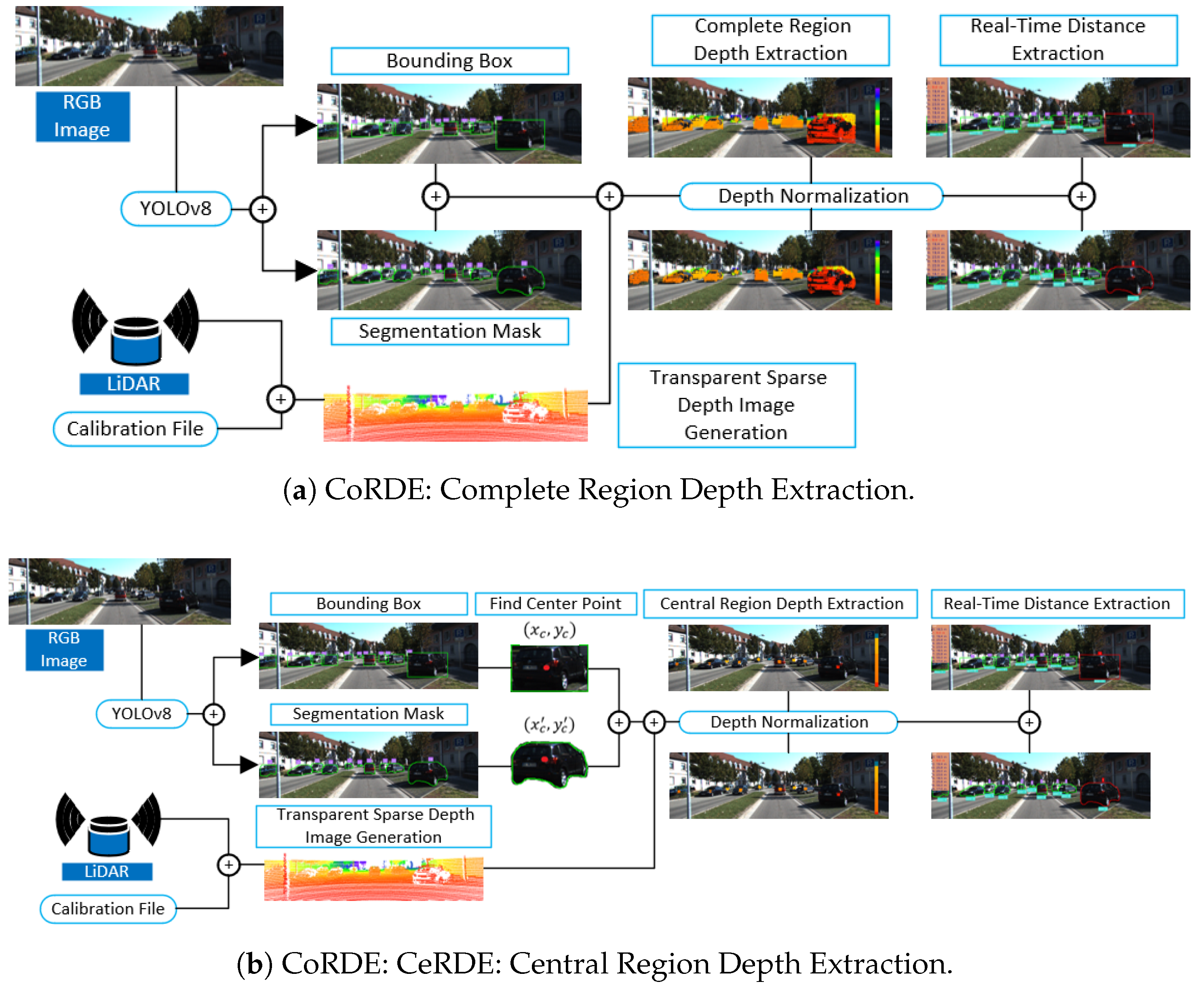
The CoRDE pipeline fuses the camera and LiDAR point clouds to generate accurate depth estimates for object detection and segmentation, as shown in Figure 1a.

Initially, a transparent sparse depth map is created from the LiDAR point cloud using the provided calibration file. The YOLOv8 model is applied to the image to detect objects, outputting bounding box coordinates and segmentation masks. These outputs are then mapped onto the transparent sparse depth map. For each detected object, the pipeline extracts the pixel color values within the full bounding box and segmentation region. The minimum depth value within these regions is selected to represent the object’s distance. See Figure 1a for an overview of the CoRDE pipeline.

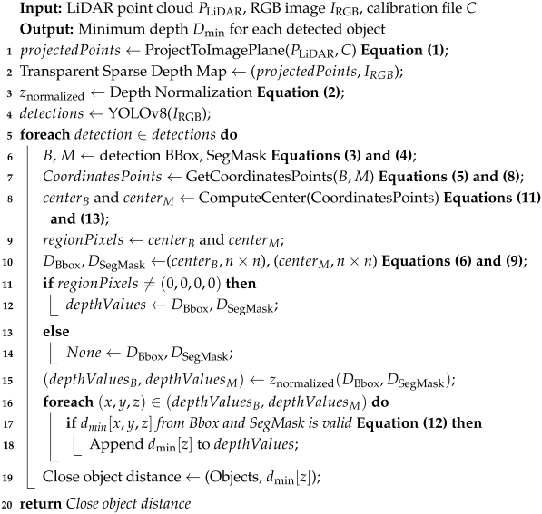
The CeRDE pipeline also combines camera and LiDAR point clouds to estimate object distances, as shown in Figure 1b. A transparent Sparse Depth Image is first generated using the calibration data and LiDAR point cloud. YOLOv8 provides the bounding box and the segmentation mask coordinates. For each detected object, central regions are calculated in the bounding box. Around the central point, a local area of size (n × n) is extracted in the transparent Sparse Depth Image. The minimum value of pixels within this area is selected as the depth distance of the object. A similar process is applied to the segmentation mask. The central point of the segmentation polygon is located, and the object distance is extracted from the Transparent Sparse Depth Image. This approach focuses on the object’s central region to reduce the influence of outlier pixels and noise. An illustration of the CeRDE pipeline is provided in Figure 1b.

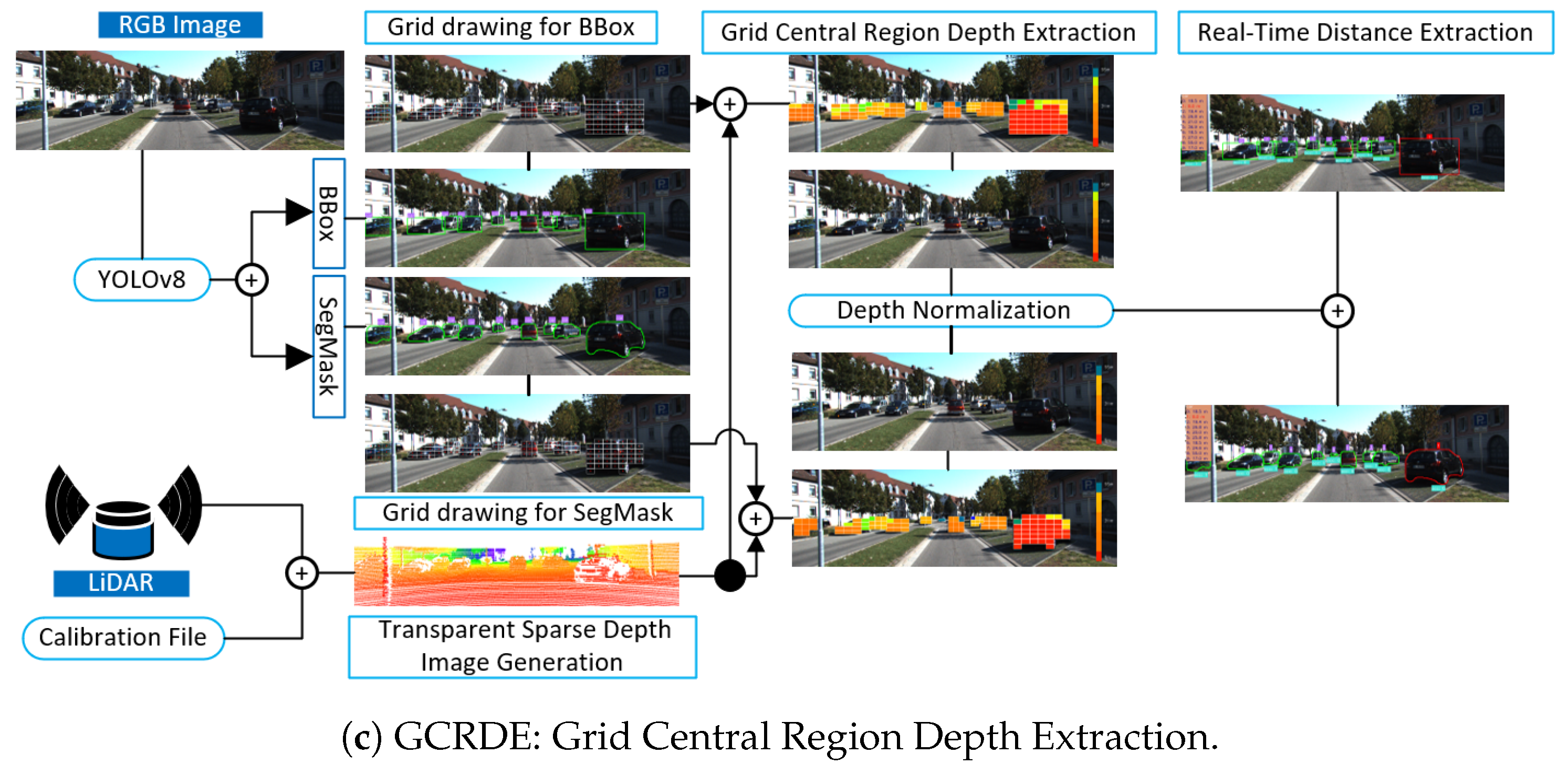
The GCRDE pipeline extends the CeRDE approach by applying a grid cell strategy across each object, as shown in Figure 1c. After creating the transparent Sparse Depth Image using the LiDAR point cloud and the calibration file, YOLOv8 is used for object detection. For each detected object, a grid is overlaid on the bounding box or segmentation mask. The center point of each grid cell is identified, and a (n × n) pixel region is extracted around it. The minimum depth value from each region is collected. These minimum values are grouped by similar depth values, and the group with the highest count indicates the estimated object distance. This grid-based approach investigates multiple grid cell regions, hence it increases robustness by reducing the impact of noise and missing depth data. A demonstration of the GCRDE pipeline is provided in Figure 1c.

In this work, we propose CoRDE, CeRDE, and GCRD novel pipelines that share a YOLOv8 detection method and transparent Sparse Depth Image (produced by LiDAR point cloud) but differ significantly in their depth extraction strategies, as shown in

Table 1. Comparison of the depth estimation pipelines and their estimation strategies.

Pipeline	Fusion Strategy	Region Type	Estimating Distances
CoRDE	Full Region	Entire Region	Minimum value in the region
CeRDE	Central point	n × n region around the center point	Minimum in n × n region
GCRDE	Grid + Central point	n × n regions around grid cell centers	The most frequent depth group

. Each pipeline introduces a novel approach for combining image features with sparse LiDAR data to enhance object-level distance estimation.

3.1.1. Transparent Sparse Depth Image Generation

The sparse depth map is generated by converting the 3D LiDAR point cloud into a 2D depth image, with the depth of each point consisting of pixel color values. Our transparent Sparse Depth Image process creates a map image in which depth information is present in each pixel that corresponds to a LiDAR point, while other pixels remain transparent. The core idea is to convert LiDAR data into a transparent Sparse Depth Image enabling its seamless integration with the image captured by the camera. To project the LiDAR points into the 2D image plane, it is used the intrinsic and extrinsic parameters of both sensors in the calibration file. The intrinsic parameters have the camera’s focal length and main point. The extrinsic parameters have the relative position and orientation between the LiDAR sensor and the camera. These parameters are utilized to compute and map the 3D points from the LiDAR into the 2D coordinate system of the camera.

$$\left[\begin{array}{c}u\\ v\end{array}\right]={\mathbf{R}}_{\mathrm{rect}}^{\left(0\right)}\ast \left[\begin{array}{c}\mathbf{R}\end{array}\right]\ast \left[\begin{array}{c}\mathbf{T}\end{array}\right]\ast {\left[\begin{array}{cccc}X& Y& Z& 1\end{array}\right]}^{\top }$$

(1)

Equation (1) shows the projection matrix between a 3D LiDAR point and its corresponding 2D pixel coordinate in the image. Here, (u, v) represent the pixel coordinates, while ${\mathbf{R}}_{\mathrm{rect}}$ is a rectification matrix. [R, T] represent the rotation matrix and translation vector that align the coordinate systems of the LiDAR and camera. Finally, [x, y, z, i] denote the coordinates of points in 3D LiDAR data [26].

3.1.2. Depth Normalization and Mapping

LiDAR-color normalization refers to the process of mapping LiDAR data, often height or intensity values from a point cloud, to color values for visualization purposes [27]. Since LiDAR data consist of points in 3D space, typically represented as [x, y, z, i] and sometimes intensity, it lacks direct color information. To visualize these points meaningfully in 2D or 3D maps, it is essential to normalize certain attributes, such as height z or intensity, and map them to color values. This process helps in creating colorized point clouds or height maps where different heights or intensities are represented by different colors [28,29]. In addition, the normalization process involves scaling the attribute values into a specific range, from 0 to 255, to ensure that the color representation is accurate and meaningful. By doing this, the visual output becomes more intuitive, allowing for easy interpretation of the data based on color changes. This normalization is performed using the following equation:

$$z_{normalized}={\displaystyle \frac{(z-z_{min})}{(z_{max}-z_{min})}}x(c_{max}-c_{min})+c_{min}$$

(2)

where $z_{min}$ and $z_{max}$ represent the minimum and maximum elevation values, while $c_{min}$ and $c_{max}$ define the range of colors used in the mapping. By applying this transformation, LiDAR data can be visualized effectively in applications such as colorized point clouds and height maps, improving data interpretation and analysis.

Figure 2 illustrates the pixel color range from 0 to 255. A pixel value of 0 corresponds to 0 m, while a pixel value of 255 represents 255 m. The transparent sparse depth map consists of x, y, and z points, where the z values are derived using this scale. After extracting the pixel from the transparent sparse depth map, Equation (2) is applied to calculate the distance corresponding to each pixel. Since there are no pixel colors representing intermediate values, the margin of error relative to the actual value is $\pm 1$ m.

Figure 3a presents transparent Sparse Depth Images, generated using Equation (1). The pixel colors represent different distance ranges. Black pixels indicate the closest points. Gray pixels represent slightly farther distances, followed by light gray pixels, which are even more distant. An even lighter shade of gray signifies points that are significantly farther away. Finally, white pixels denote the farthest distances. The transparent sparse depth map becomes unclear when projected onto the RGB image. To enhance clarity, the depth map was colorized for better visualization, as shown in Figure 3b. In this paper, the results are presented in color.

3.2. YOLOv8 Object Detection Method

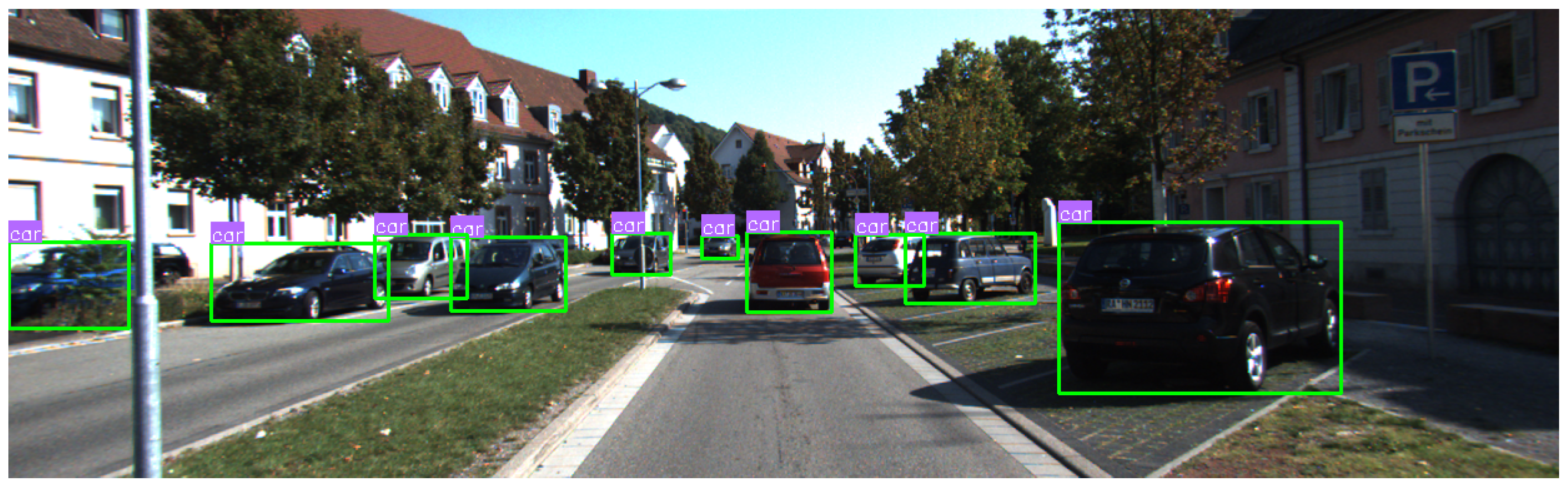
YOLOv8 excels in providing accurate and efficient bounding box predictions, which are critical for object localization in real-time applications. The bounding box output in YOLOv8 is represented by four key coordinates: the center (x, y), width (w), and height (h). These parameters define the region in the image where an object is detected. YOLOv8 improves upon earlier versions by using a more advanced architecture that enhances the precision of the predicted bounding box, even in crowded or complex scenes. The coordinates of the bounding box for the N-th object are given by the detection of an object in an image, and its bounding box is defined as follows:

$$YOL{O}_{\mathrm{Bbox}}=\{(x_{1_0},y_{1_0},x_{2_0},y_{2_0}),\dots \dots ,(x_{1_N},y_{1_N},x_{2_N},y_{2_N})\}$$

(3)

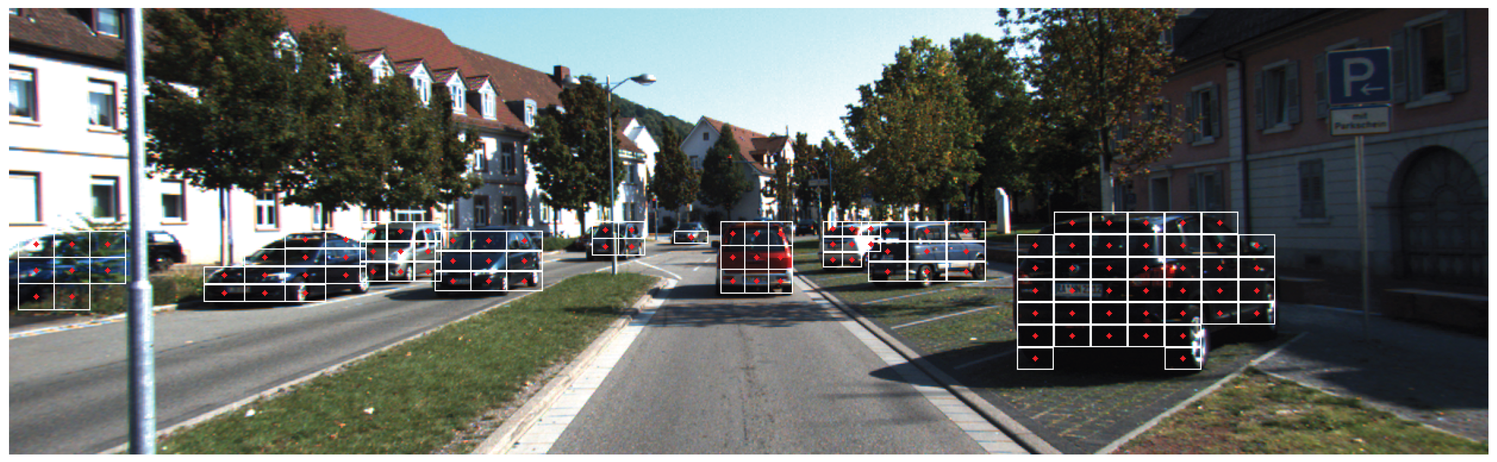
where $(x_{min},y_{min})$ and $(x_{max},y_{max})$ represent the top-left and bottom-right coordinates of the bounding box. Figure 4 shows the bounding box outputs from YOLOv8 for each object.

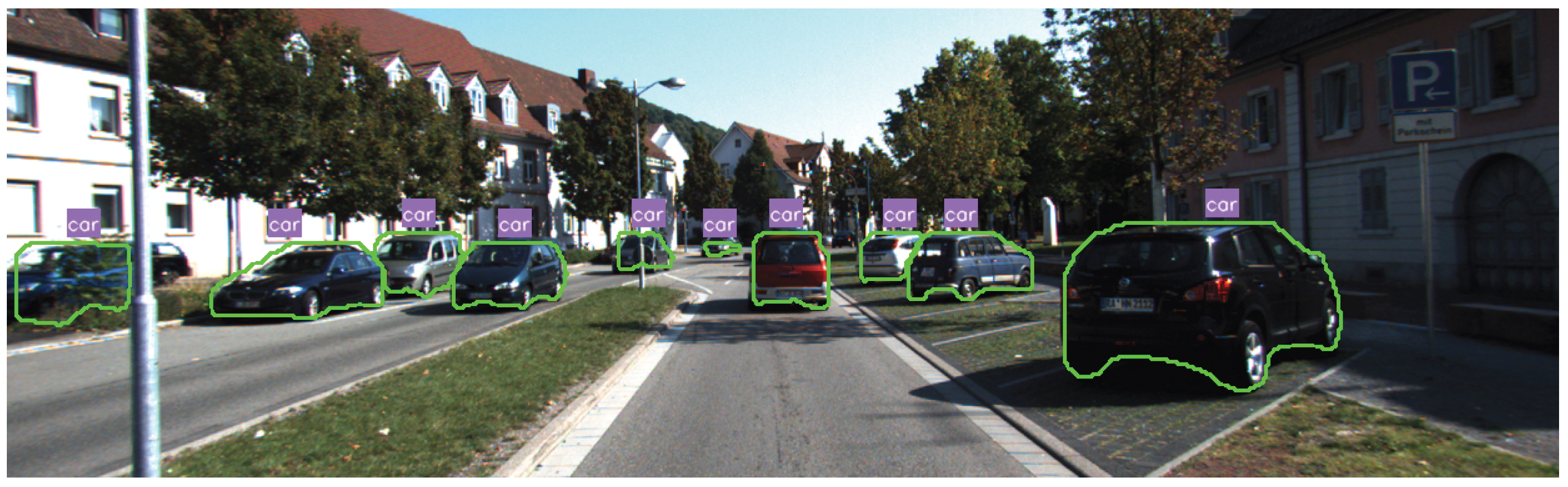
In addition to the bounding box prediction, YOLOv8 provides segmentation masks, which are critical for more detailed object recognition tasks. Unlike traditional bounding box-based models that only identify the object’s location, YOLOv8 offers pixel-level segmentation, making it capable of capturing the precise shape of the object within the bounding box. This segmentation mask is generated by predicting pixel-wise classification for each object within the bounding box, providing a more accurate delineation of object boundaries. If the mask consists of a series of points ($x_i$, $y_i$), it can be represented as a polygon, and YOLOv8 provides a segmentation mask as a set of N points:

$$YOL{O}_{\mathrm{SegMask}}=\{(x_0,y_0),(x_1,y_1),(x_2,y_2),\dots \dots ,(x_N,y_N)\}$$

(4)

Figure 5 illustrates the segmentation mask polygons across multiple objects, which are generated by YOLOv8.

3.3. LiDAR-Camera Object Distance Extraction

LiDAR point cloud has an [x, y, z, i] value and these x, y values define the point in the position on the LiDAR scanner area, and z defines the distance between the point and LiDAR origin points.

3.3.1. Complete Region Depth Extraction

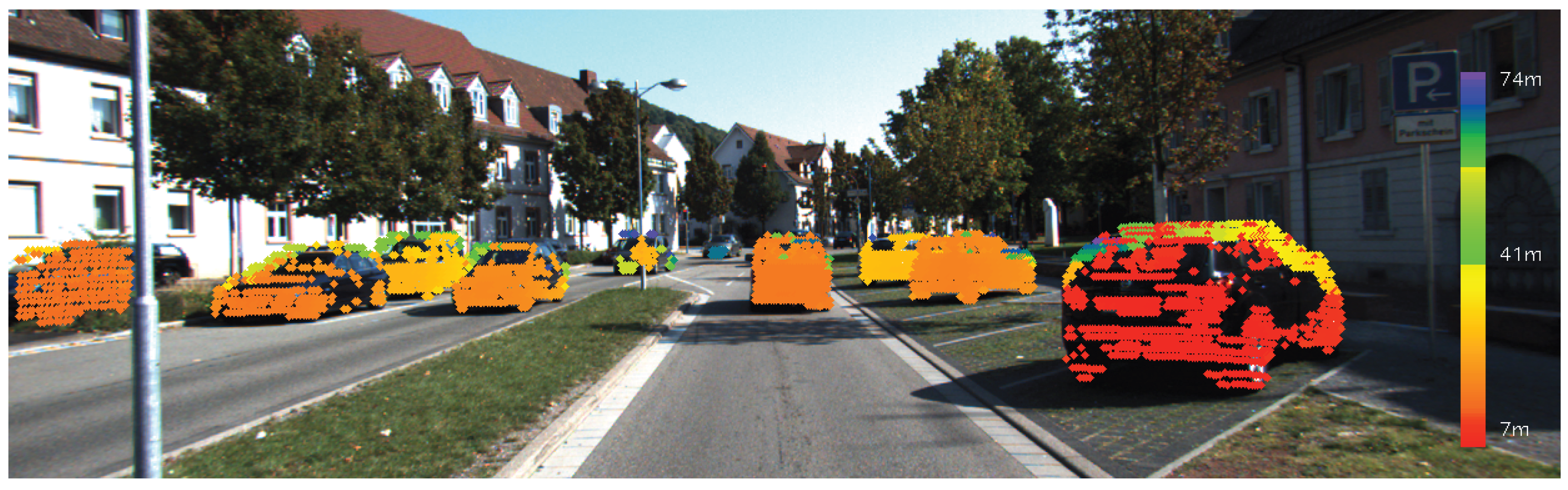
This CoRDE extracts depth values from within the bounding box and segmentation mask. It has two primary stages. Initially, all pixel values within the bounding box and segmentation mask are extracted from the transparent Sparse Depth Image. Next, the minimum pixel intensity value is then identified, as smaller depth values signify proximity to objects. The minimal intensity value is thereafter correlated to its respective distance by a predetermined normalization function.

The bounding box (bbox) is a rectangular area surrounding the detected object. It is typically provided by object detection models and has been defined by four coordinates. $x_{min}$, $x_{max}$, $y_{min}$, and $y_{max}$ represent the left, right, upper, and lower bounds, respectively. Every pixel within this rectangle is regarded as belonging to the object.

$$Bbox=\{(x,y)\mid x_{min}\le x\le x_{max},y_{min}\le y\le y_{max}\}$$

(5)

The pixel coordinates of the bounding box frame generated by the object detection method are located on the transparent Sparse Depth Image ($I(x,y)$). Then, the depth values in this frame are subsequently extracted. Each extracted pixel value contains a depth value.

$$D_{\mathrm{Bbox}}=\{I(x,y)\mid (x,y)\in Bbox\}$$

(6)

To determine the actual distance to the object from the depth data, the predetermined normalization function is employed, and the minimal depth within the bounding box is computed using Equation (7).

$$d_{\min }^{\mathrm{Bbox}}=\underset{(x,y)\in Bbox}{min}I(x,y)$$

(7)

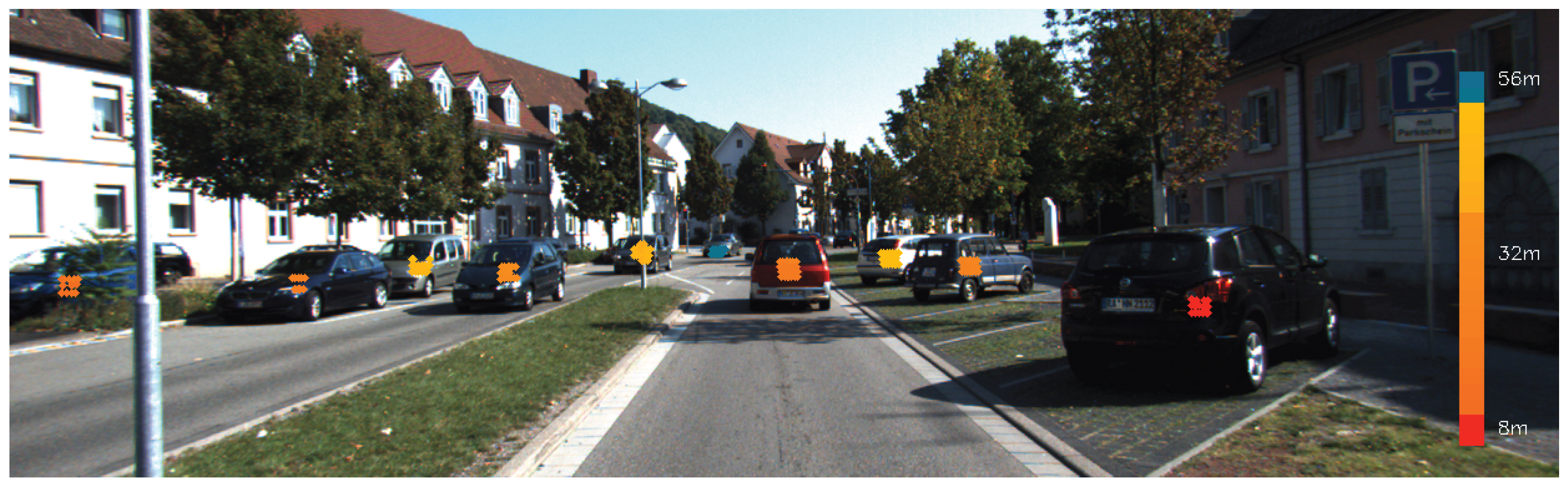
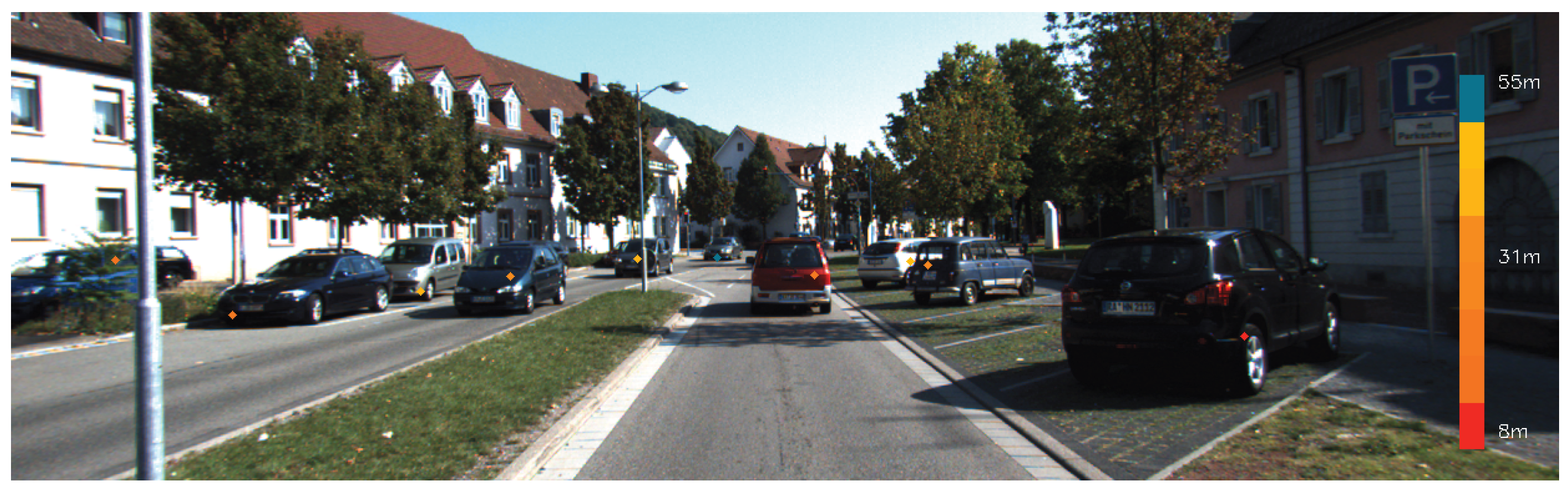
The transparent Sparse Depth Image (shown in Figure 3a) and the RGB image (as shown in Figure 3b) have been fused as inputs for the Complete Region Depth Extraction. The output image displays the depth value points for each object, as illustrated in Figure 6.

A segmentation mask (SegMask) is a classification map that is presented pixel-by-pixel, determining which pixels are associated with the item. The shape of the object that it offers is more precise than that of a bounding box. The segmentation mask is represented as follows:

$$SegMask(x,y)=\left\{\begin{array}{cc}1,\hfill & \mathrm{if}(x,y)\mathrm{is}\mathrm{part}\mathrm{of}\mathrm{the}\mathrm{object}\hfill \\ 0,\hfill & \mathrm{otherwise}\hfill \end{array}\right.$$

(8)

The segmentation mask with $(x,y)$ coordinates in the shape of a polygon is provided by the semantic object detection method. The mask, called SegMask, is a frame line containing the object. Polygon coordinates are found in the transparent Sparse Depth Image ($I(x,y)$). After that, the pixel points contained within the polygon are extracted from the transparent Sparse Depth Image. Each extracted pixel has a depth value that corresponds to it.

$$D_{\mathrm{SegMask}}=\{I(x,y)\mid SegMask(x,y)=1\}$$

(9)

A predefined normalization function is used to estimate the distance from the depth data to the object. Since each pixel extracted from the segmentation mask area belongs to the object, Equation (10) is utilized to calculate the estimated distance.

$$d_{\min }^{\mathrm{SegMask}}=\underset{(x,y)\in D_{\mathrm{SegMask}}}{min}I(x,y)$$

(10)

The depth values of each object are fused with the semantic segmentation results of the object detection method with the transparent Sparse Depth Image. In Figure 7, the extracted pixel points are colored to provide better clarity and comprehension.

Table 2. Comparison of bounding box and segmentation mask for complete region depth extraction.

Feature	Bounding Box	Segmentation Mask
Shape Precision	Rectangular	Exact object shape
Background Noise	Includes background pixels	Only object pixels
Distance Accuracy	May include far pixels	More precise

shows that the bounding box provides a rectangular shape, which may include background pixels, whereas the segmentation mask offers the exact shape of the object, reducing background noise.

As a result, the segmentation mask provides more precise depth values by focusing only on the object’s pixels, while the bounding box may introduce inaccuracies due to the inclusion of pixels at varying depths.

3.3.2. Central Region Depth Extraction

The CeRDE estimates the object’s distance by choosing a single representative point instead of evaluating all pixels within the bounding box and the segmentation mask. This approach greatly reduces computational complexity while it consistently increases the accuracy of the depth estimation. The bounding box that is shown in Figure 8a is a rectangular box delineating the detected object. The center point of the bounding box is determined by calculating the midpoint between its minimum and maximum coordinates along both the x-axis and y-axis.

The coordinates $x_{min}$, $y_{min}$, $x_{max}$, and $y_{max}$ provided by the object detection algorithm are used to determine the center point within the bounding box. The coordinates of the central point ($x_c$, $y_c$) are computed using Equation (11).

$$x_c={\displaystyle \frac{x_{min}+x_{max}}{2}},y_c={\displaystyle \frac{y_{min}+y_{max}}{2}}$$

(11)

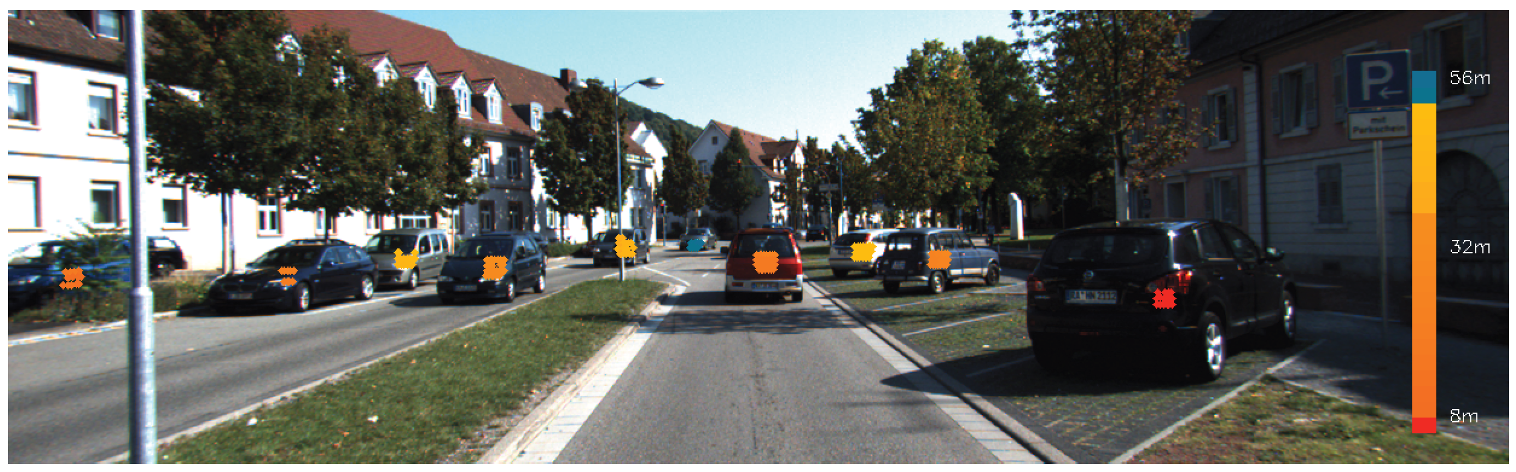
Once the central point is identified, it is mapped onto the transparent Sparse Depth Image to extract the corresponding depth value. However, due to the low resolution of the LiDAR point clouds, the exact depth value at ($x_c$, $y_c$) may not always be available.

To address this issue, a (n × n) pixel rectangular area is delineated around ($x_c$, $y_c$), ensuring that at least a few depth values can be obtained from the Sparse Depth Image. The depth values of all eligible pixels within this rectangle are extracted and the minimum depth value is chosen as the estimated distance of the object using Equation (12).

$$d_{\min }=min\{I(x,y)\mid (x,y)\in R\}$$

(12)

where R represents the set of pixels inside the (n × n) rectangular area, and $I(x,y)$ is the depth value at pixel ($x_c$, $y_c$) in the transparent Sparse Depth Image. Depth values associated with each object are represented by color pixels to be clear in Figure 9.

Segmentation masks provide a more precise depiction of the object by delineating the actual shape of the object, in contrast to bounding boxes, which only provide an approximate representation of the object’s localization. To extract the depth information that is meaningful, the segmentation mask is converted into a polynomial. The central point of the segmentation mask is computed by averaging the coordinates of the polygon using Equation (13), ensuring that the estimated center accurately represents the object’s true position instead of relying on the center of the bounding box. N is the total number of pixels in the polynomial, while ($x_i$, $y_i$) are the coordinates of each polynomial pixel, as defined in Equation (13).

$$x_c^{\prime }={\displaystyle \frac{1}{N}}\sum _{i=1}^N{x}_i,y_c^{\prime }={\displaystyle \frac{1}{N}}\sum _{i=1}^N{y}_i$$

(13)

The coordinates ($x_c^{\prime }$, $y_c^{\prime }$) are determined and then the depth value is extracted from the transparent Sparse Depth Image at this coordinate. However, due to the limited space of LiDAR data, the precise depth value at ($x_c^{\prime }$, $y_c^{\prime }$) may be missing. To resolve this, a small search region around (n × n) is examined and the minimum depth value in this region is found using Equation (12). The selected depth value from the transparent Sparse Depth Image is illustrated in color in Figure 10.

The comparison highlights that both approaches achieve high shape precision, with exact center point determination ($x_c$, $y_c$) for bounding box and ($x_c^{\prime }$, $y_c^{\prime }$) for segmentation mask. In addition to this, they efficiently reduce background noise by taking into consideration only object pixels, which results in clearer data extraction.

Additionally, both methods exhibit good accuracy when it comes to measuring distance. As a consequence of this, their performance is comparable in terms of precision, noise filtering, and measurement accuracy, as summarized in

Table 3. Comparison of bounding box and segmentation mask for Central Region Depth Extraction.

Feature	Bounding Box	Segmentation Mask
Shape Precision	Extract ($x_c$, $y_c$) Point	Extract ($x_c^{\prime }$, $y_c^{\prime }$) Point
Background Noise	Only object pixels	Only object pixels
Distance Accuracy	More precise	More precise

.

3.3.3. Grid Central Region Depth Extraction

The GCRDE is designed to enhance the accuracy of object distance estimation. This approach improves the object detection process by employing both bounding boxes and segmentation masks to improve depth estimates. Once an object is detected in an image, a grid is drawn over it to divide it into smaller regions for more precise depth extraction. The KITTI dataset provides occlusion levels and difficulty information based on object height. Depending on the information, objects with a bounding box or a segmentation mask height of a minimum of 25 pixels fall under the hard or moderate category. In this case, no grid is drawn, and only the central point of the entire bounding box or the segmentation mask is used. Equation (14) shows that $y_{\min }$ and $y_{\max }$ are determined by finding the top and bottom of the bounding box and the segmentation mask.

$$height=y_{\max }-y_{\min }>25$$

(14)

If the object’s bounding box or segmentation mask height exceeds a minimum of 40 pixels, a $m\times m$ grid is created over the object, and the length and width of each grid cell are calculated using Equation (15).

$$w_{cell}={\displaystyle \frac{x_{max}-x_{min}}{m}},h_{cell}={\displaystyle \frac{y_{max}-y_{min}}{m}}$$

(15)

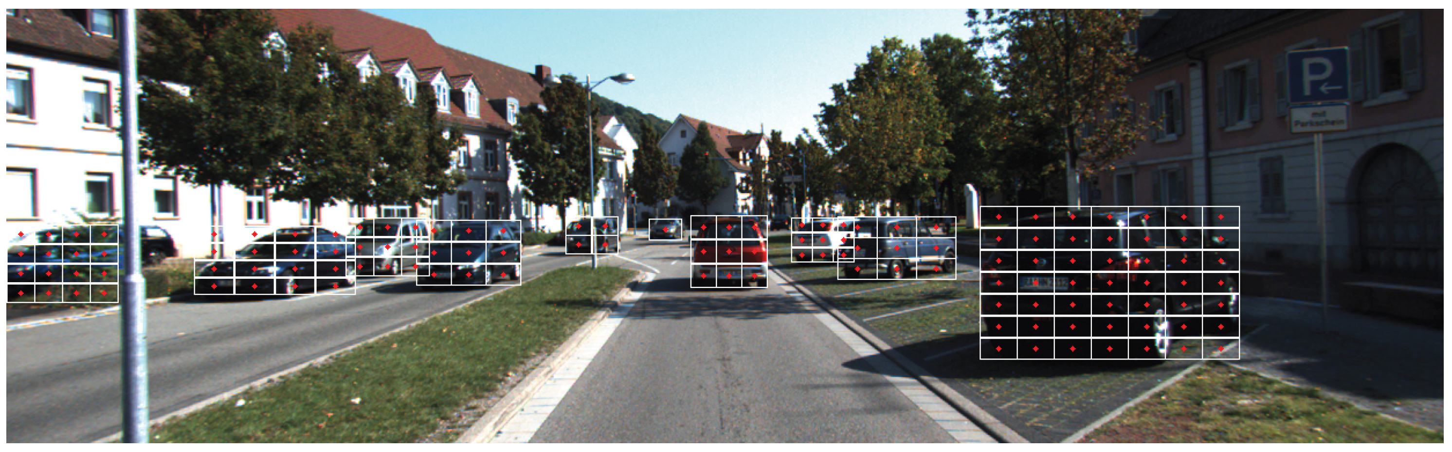
Since the bounding box contains background pixels, direct depth extraction from its center can lead to inaccuracies. To prevent this, each grid cell’s central point is calculated, ensuring a more localized and precise estimation. The central point of each grid cell $(x_{cel{l}_c},y_{cel{l}_c})$ is computed as follows:

$$x_{cel{l}_c}=x_{min}+\left(i+{\displaystyle \frac{1}{2}}\right)w_{cell},y_{cel{l}_c}=y_{min}+\left(j+{\displaystyle \frac{1}{2}}\right)h_{cell}$$

(16)

where $i,j$ are the row and column indices of the grid cells, and they range from 0 to $m-1$, as given by $i,j\in \{0,1,\dots ,m-1\}$. The grids shown in Figure 11 were generated using the bounding box coordinates of each object, and then the center point of each grid cell was calculated based on these grids.

Due to the lower resolution of the transparent sparse depth map, an (n × n) pixel search area is used around each cell’s central point. If depth values exist within this region, the minimum depth value is selected using Equation (12) to estimate the object distance. This process is repeated for each grid cell, ensuring that depth values are captured at multiple points in the object.

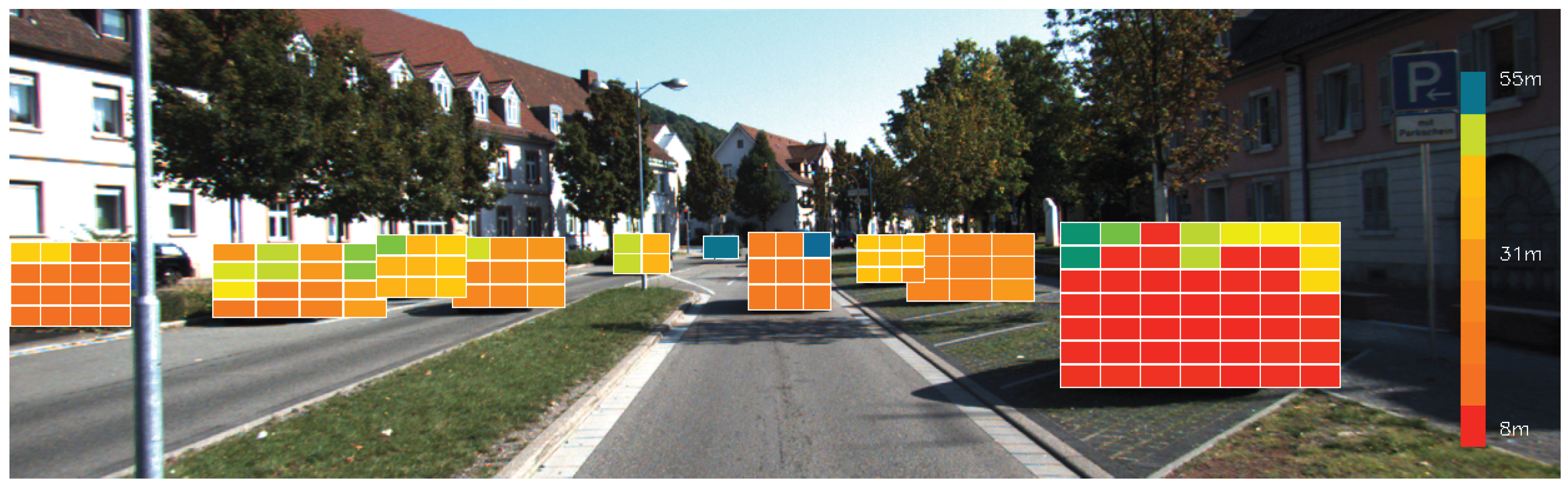
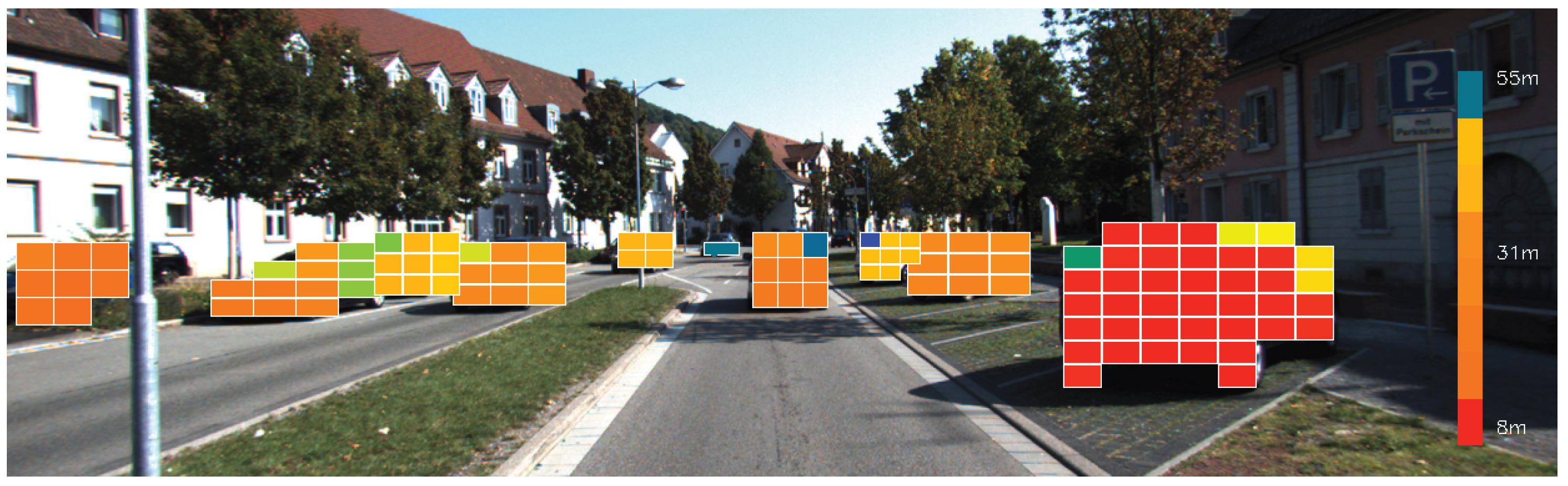
Figure 12 illustrates the grid cells drawn on each object, with colors representing the distance measurement of these cells. Even though some grid cells belong to the same object, they appear in different colors. This variation occurs because object detection methods create bounding boxes that not only encompass the object itself but also capture parts of the surrounding background. Figure 12 shows how irrelevant background fields can influence the detected object distance.

Each depth value that is extracted corresponds to a specific grid center point. In order to ensure consistency and robustness, a grouping process is applied. This process involves counting the number of grid cells that share the same depth value. The depth value that has the largest occurrence is then chosen as the object’s final estimated distance. By extracting multiple depth values ($d_{grid}=\{d_1,d_2,\dots ,d_{m^{\prime }}\}$, where $m^{\prime }$ is the total number of grid center points, from the object and selecting the most dominant one, this method improves accuracy and ensures a more reliable object distance measurement. The regions of the objects corresponding to the distance information derived from the depth values of the most dominant grid cells are illustrated in Figure 13.

When 3D LiDAR points from different parts of large objects, such as vehicles, buses, or trucks, are projected onto a 2D plane, the points are concentrated in a restricted area within the image. This causes errors in the depth information extracted from the transparent Sparse Depth Image, utilizing data from object detection methods. Despite the extraction of depth values utilizing the segmentation mask frame that completely covers the objects, Figure 14 illustrates that background noise remains. To reduce background noise, grids are generated to fully cover each object, utilizing the segmentation mask information along with Equations (14)–(16). The center points of the grid cells corresponding to each object are then determined, as illustrated in Figure 15.

The depth values for each grid cell within the (n × n) area around its center point are extracted from the transparent Sparse Depth Image. These depth values are then utilized in Equation (12) to compute the distance information for each grid cell. The retrieved distance information is visualized in Figure 14.

For each grid cell, the extracted depth values from the object are grouped and stored. The most frequent depth values are then used to determine the object’s distance. The distance corresponding to the most common group is selected as the object’s final distance. By utilizing the segmentation mask, which accurately defines the object boundaries, errors caused by irrelevant background pixels are significantly reduced. This results in more precise and reliable distance estimations, especially for complex objects. The locations of the depth information extracted from the objects are illustrated in Figure 16.

The bounding box captures more background noise, whereas the segmentation mask reduces it but does not eliminate it entirely. In contrast, the grid Central Region Depth Extraction method effectively removes background noise, ensuring precise depth estimation for both the bounding box and segmentation mask approaches. Despite these variations, both methods demonstrate high performance in precision, noise filtering, and overall measurement accuracy, as summarized in

Table 4. Comparison of bounding box and segmentation mask for Grid Central Region Depth Extraction.

Feature	Bounding Box	Segmentation Mask
Shape Precision	Rectangular grid	Exact object shape grid
Background Noise	Includes background pixels	Only object pixels
Distance Accuracy	Much more precise	Much more precise

.

4. Evaluation

All implementations were executed on a server computer with an Intel^® Xeon^® 2.20 GHz CPU, 64 GB of RAM, and an NVIDIA GeForce RTX 3090 GPU with 24 GB of VRAM, running Ubuntu 20.04.6. The implementations were developed in Python 3.10 using PyTorch 2.2.2, CUDA12, OpenCV 4.9, and Numpy 1.26.4. All timing measurements were performed on this server without parallelization or GPU-specific acceleration.

4.1. Dataset

The KITTI (Karlsruhe Institute of Technology and Toyota Technological Institute) object detection benchmark consists of 7481 training images and 7518 test images, along with corresponding point cloud data calibration files and annotations. It includes five object categories, which are person, bicycle, car, bus, and truck. The dataset also defines three levels of occlusion difficulty, which are easy, moderate, and hard, based on object visibility, bounding box height, and truncation. The easy category requires a minimum bounding box height of 40 pixels, with objects being fully visible and a maximum truncation of 15 percent. The moderate category includes objects with a minimum bounding box height of 25 pixels, partial occlusion, and up to 30 percent truncation. The hard category consists of objects with at least 25 pixels in bounding box height and significant occlusion, making them difficult to see, and up to 50 percent truncation. These difficulty levels ensure a comprehensive evaluation of object detection models under various real-world conditions [1].

Table 5. The KITTI object detection benchmark.

Image Feature	Easy	Moderate	Hard
Max. occlusion level:	Fully visible	Partly occluded	Difficult to see
Min. bounding box height:	40 Px	25 Px	25 Px
Max. truncation:	15	30	50
Number of Object:	14550	6428	3511

shows the specific criteria for each difficulty level, including the maximum occlusion level, minimum bounding box height, maximum truncation, and the number of objects in each category.

4.2. Bounding Box Similarity Check

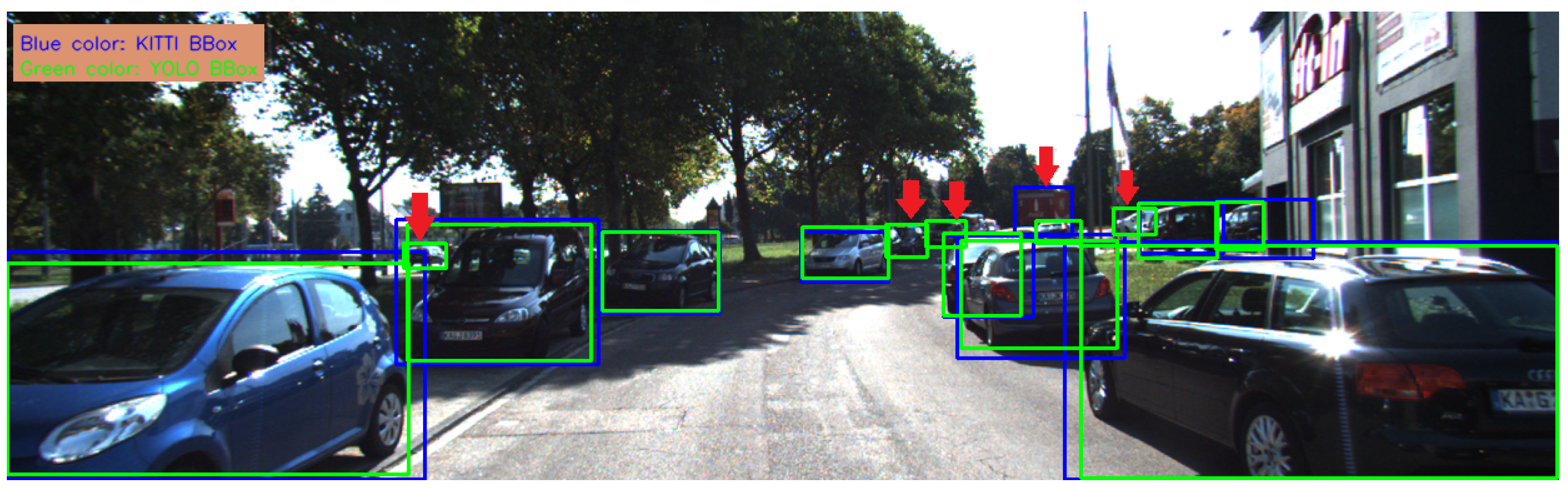
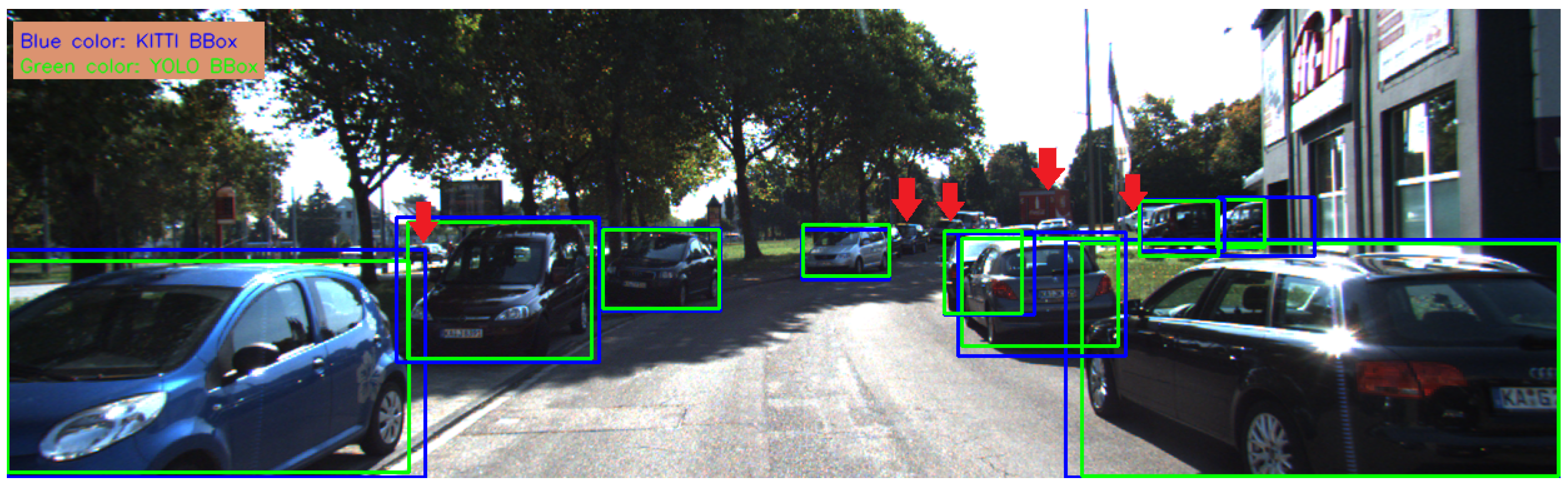
The KITTI dataset provides occlusion values for each object. In this study, the time and the occlusion value required to estimate the distance of each object were evaluated to measure the efficiency of the methods. YOLOv8 was used as the object detection method, and it provided the bounding box and the segmentation mask for detected objects, including persons, bicycles, cars, buses, and trucks. To ensure an accurate evaluation, the bounding box information of objects with occlusion values from the KITTI dataset must match the bounding box information provided by YOLOv8. Figure 17 illustrates the bounding boxes drawn in the image using coordinate information from both KITTI and YOLOv8.

As shown in Figure 17, YOLOv8 detects more objects, whereas the KITTI dataset provides fewer object annotations and includes information about a foreign object outside the defined categories of person, bicycle, car, bus, and truck. Furthermore, while YOLOv8’s bounding box coordinates closely match the exact size of the object, the KITTI dataset’s annotation bounding boxes tend to be larger than the actual object size. To address this discrepancy and ensure a high-accuracy evaluation, similarity checks were performed between the bounding box annotations from the KITTI object detection benchmark dataset and the bounding boxes provided by YOLOv8 for each object in the image.

$$\mathrm{KITTI}=(x_1^1,y_1^1,x_2^1,y_2^1),and\mathrm{YOLOv}8=(x_1^2,y_1^2,x_2^2,y_2^2)$$

(17)

The similarity between the KITTI and YOLOv8 bounding boxes was compared by computing the absolute differences between their corresponding bounding box coordinates. The differences in the top-left coordinates were calculated as $\Delta x_1=|x_1^1-x_1^2|$ for the x-coordinates and $\Delta y_1=|y_1^1-y_1^2|$ for the y-coordinates. Similarly, the differences in the bottom-right coordinates were calculated as $\Delta x_2=|x_2^1-x_2^2|$ for the x-coordinates and $\Delta y_2=|y_2^1-y_2^2|$ for the y-coordinates. These differences helped to quantify the spatial deviation between two bounding boxes, allowing a threshold-based similarity condition to be defined.

$$\mathrm{is}\_\mathrm{similar}(\mathrm{KITTI},\mathrm{YOLOv}8)=\left\{\begin{array}{cc}\mathrm{True},\hfill & \mathrm{if}\Delta x_1\le T\mathrm{and}\Delta y_1\le T\hfill \\ \hfill & \mathrm{and}\Delta x_2\le T\mathrm{and}\Delta y_2\le T\hfill \\ \mathrm{False},\hfill & \mathrm{otherwise}\hfill \end{array}\right.$$

(18)

To determine whether two bounding boxes were similar, a predefined threshold (T) was applied to the coordinate differences. The similarity condition required that the absolute differences between the corresponding coordinates of the two bounding boxes remain within this threshold. When all these conditions were satisfied, the bounding boxes were considered similar. Mathematically, this was expressed in Equation (18).

Figure 18 shows the refined bounding box data after the elimination of irrelevant objects. All KITTI and YOLO bounding boxes have been successfully matched, ensuring consistency between the data. In this way, the final bounding box and segmentation mask information is optimized for input into our methods.

4.3. Truth Table Generation for Object Distance Measurement with YOLO Segmentation and LiDAR Clustering

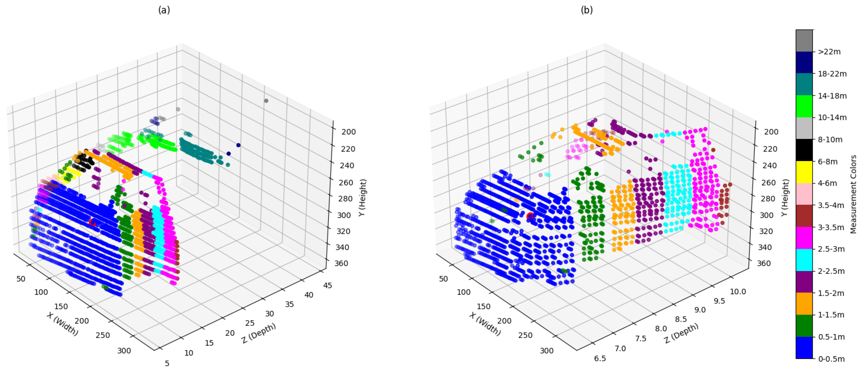
The KITTI object detection benchmark dataset comprises annotation object coordinates, and the objective of this part was to generate a truth table for comparison with our method’s distance measurements. YOLO object detection was employed to acquire object segmentation masks. The coordinates of these segmentation masks were compared with the KITTI object annotation. Afterward, the matched annotations were used to verify whether the LiDAR points were inside the segmentation mask of the detected object. If a LiDAR point was located within the mask, the (x, y, z) coordinates were stored. The collected data comprised LiDAR points associated with things, along with extraneous noise and irrelevant LiDAR information. Clustering was employed to eradicate this noise. Figure 19 illustrates that the clustering comprises 15 types.

After that, the clustering was focused on objects within a range of 0 to 2.5 m. The nearest cluster was located, and the minimum value was retrieved to ascertain the object’s distance. Ultimately, the truth table was generated for several item categories, encompassing pedestrians, bicycles, cars, buses, and trucks. The occlusion levels were categorized into four classifications, respectively, 0, 1, 2, and 3.

Table 6. Number of objects classified as Easy, Moderate, Hard, and Unknown in the Truth Table.

Image Feature	Person	Bicycle	Car	Bus	Truck
Easy	2963	62	12410	245	768
Medium	785	45	7387	114	600
Hard	166	6	4164	14	271
Unknown	210	15	859	65	285

presents the distribution of objects in the truth table categorized into four difficulty levels: Easy (fully visible objects), Moderate (partially occluded objects), Hard (highly occluded or difficult-to-see objects), and Unknown (objects with uncertain visibility or occlusion status). This classification helps in analyzing object detection performance under varying visibility conditions.

4.4. Quantifying Error for Bounding Box and Segmentation Mask Depth Predictions

Although the mean squared error (MSE) [17,30] is commonly used in research, the root mean squared error (RMSE) [7,31,32] is chosen in this study due to its interpretability in the same unit as the original data, which in this case is distance (meters). RMSE provides a more sensitive measure of prediction accuracy, making it particularly useful for evaluating the performance of depth estimation. The process begins by extracting the object distances separately using the bounding box and segmentation mask data. Afterward, the truth table is used to compute the RMSE for both the bounding box and segmentation mask. The truth table provides the actual ground truth distances for comparison, while the distances obtained from the predicted bounding box and segmentation mask are compared separately. The RMSE for the bounding box and segmentation mask is then calculated using the following formula:

$$RMSE=\sqrt{{\displaystyle \frac{1}{N}}\sum _{i=1}^N{(y_i-{\widehat{y}}_i)}^2}$$

(19)

where $y_i$ represents the actual distance from the truth table for the i-th data point, ${\widehat{y}}_i$ represents the predicted distance either from the bounding box or the segmentation mask, and N is the total number of data points. By calculating RMSE separately for the bounding box and segmentation mask, we can quantify the error in the predicted depth values for each method. Lower RMSE values indicate better alignment between the predicted and actual distances, reflecting improved performance in the model’s depth extraction process.

4.5. Accuracy Evaluation Using Truth Table and Predicted Distances

In this study, we evaluate the performance of object distance estimation methods by comparing their predicted values with the truth table. The tested methods used the bounding box and the segmentation mask to estimate the object distance. To assess the accuracy of each method, we perform a binary comparison between predicted distances and the true values from the true table. True Positive (TP) occurs when the predicted distance matches the true value, while False Positive (FP) occurs when the predicted distance does not match the true value. Accuracy is calculated as the ratio of the number of correct predictions (TP) to the total number of predictions (TP + FP).

$$\mathrm{Accuracy}={\displaystyle \frac{TP}{TP+FP}}$$

(20)

This accuracy metric, shown in Equation (20), is computed independently for both the bounding box and segmentation mask approaches, allowing for consistent evaluation of their performance in estimating object distances.

5. Results and Discussions

This section explains the results of three different approaches: the Complete Region Depth Extraction, the Central Region Depth Extraction, and the Grid Central Region Depth Extraction. These approaches leverage object detection and distance measurement through camera-LiDAR fusion to enhance depth perception. LiDAR points were projected onto a transparent sparse depth map, which was fused with the output of the object detection method. The object detection framework provided the bounding box and the segmentation mask frame data, allowing precise depth extraction. Furthermore, the depth value extraction time and the number of extracted points for both the bounding box and the segmentation mask were recorded. These results help to evaluate the efficiency and accuracy of each method in extracting depth information.

The tables present the mean depth extraction time (in milliseconds), accuracy, and root mean squared error (in meters) for different object classes using the Complete Region Depth Extraction, the Central Region Depth Extraction, and the grid Central Region Depth Extraction. The results are shown for the bounding box and the segmentation mask under different occlusion levels (Easy, Moderate, Hard, and Unknown). Performance times presented in Figure 20, Figure 21, Figure 22, Figure 23, Figure 24, Figure 25, Figure 26, Figure 27, Figure 28, Figure 29, Figure 30, Figure 31, Figure 32 and Figure 33 were computed using the system configuration outlined in Section 4.

5.1. Comparative Analysis of Fully Visible Objects

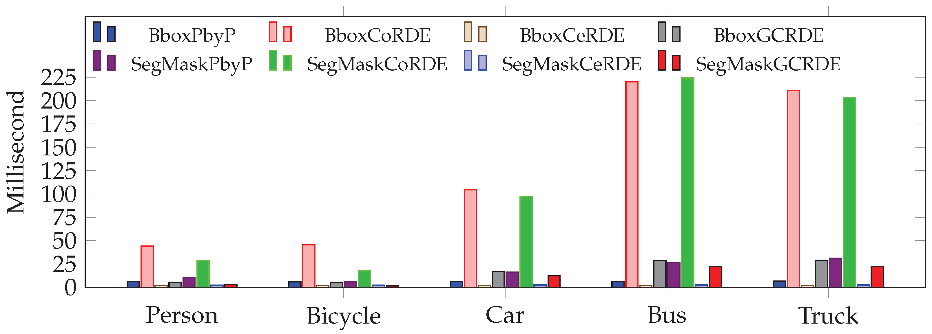
Figure 20 illustrates the average time required to perform depth extraction for fully visible objects at occlusion level 0. Among all approaches, the bounding box and the segmentation mask in CeRDE show the fastest processing times, all under 3 milliseconds. These are significantly faster than the traditional PbyP approach, which ranges from 6 to 16 milliseconds. Notably, the CoRDE approach is the slowest, especially for larger objects like buses and trucks, taking over 200 milliseconds in some cases. The GCRDE approach strikes a balance, offering faster performance than CoRDE but slower than CeRDE. These results indicate that CeRDE is the most time-efficient, making it well-suited for real-time applications.

Figure 20. This comparison shows mean depth extraction time (in milliseconds) at occlusion Levels 0 for the traditional approach: PbyP (Point-by-Point) and our proposed approaches: CoRDE (Complete Region Depth Extraction), CeRDE (Central Region Depth Extraction), and GCRDE (Grid Central Region Depth Extraction).

Figure 20. This comparison shows mean depth extraction time (in milliseconds) at occlusion Levels 0 for the traditional approach: PbyP (Point-by-Point) and our proposed approaches: CoRDE (Complete Region Depth Extraction), CeRDE (Central Region Depth Extraction), and GCRDE (Grid Central Region Depth Extraction).

Figure 21 presents the accuracy of each method in estimating depth for various object types. The segmentation mask for the CeRDE and GCRDE approaches stands out with the highest accuracy, above 88% for all objects and reaching nearly 97% for “Person”. Similarly, the bounding box for CeRDE and GCRDE also demonstrates strong performance, although slightly below their segmentation masks’ accuracies. In contrast, the CoRDE approach shows the lowest accuracy, particularly for smaller objects like bicycles. PbyP approaches perform reasonably well but lack the consistency seen in CeRDE and GCRDE. These results confirm that central and grid-based region strategies, especially with segmentation masks, significantly enhance depth estimation accuracy.

Figure 21. This comparison shows depth extraction accuracy (%) at occlusion Levels 0 for the traditional approach: PbyP (Point-by-Point) and our proposed approaches: CoRDE (Complete Region Depth Extraction), CeRDE (Central Region Depth Extraction), and GCRDE (Grid Central Region Depth Extraction).

Figure 21. This comparison shows depth extraction accuracy (%) at occlusion Levels 0 for the traditional approach: PbyP (Point-by-Point) and our proposed approaches: CoRDE (Complete Region Depth Extraction), CeRDE (Central Region Depth Extraction), and GCRDE (Grid Central Region Depth Extraction).

Figure 22 shows the RMSE values for depth estimation, where lower values indicate higher precision. The CeRDE approach again outperforms all others, with the segmentation mask and the bounding box achieving the lowest RMSEs, particularly for large objects like buses and trucks. The bounding box method in the GCRDE approach provides moderate error values. PbyP and CoRDE approaches show significantly higher RMSEs, especially for buses, where values exceed 6 m in some cases. These findings show that CeRDE delivers the most precise depth estimations.

Figure 22. This comparison shows depth extraction RMSE (in meters) at occlusion Levels 0 for the traditional approach: PbyP (Point-by-Point) and our proposed approaches: CoRDE (Complete Region Depth Extraction), CeRDE (Central Region Depth Extraction), and GCRDE (Grid Central Region Depth Extraction).

Figure 22. This comparison shows depth extraction RMSE (in meters) at occlusion Levels 0 for the traditional approach: PbyP (Point-by-Point) and our proposed approaches: CoRDE (Complete Region Depth Extraction), CeRDE (Central Region Depth Extraction), and GCRDE (Grid Central Region Depth Extraction).

The comparative evaluation of depth extraction methods under occlusion level 0 demonstrates that CeRDE, especially when combined with segmentation masks, offers the best performance overall. While the GCRDE approach provides a good compromise between speed and accuracy, it falls short of matching CeRDE’s optimal results. The CoRDE approach is both slow and less accurate, indicating that a more extensive Complete Region Depth Extraction processing may introduce noise.

5.2. Comparative Analysis of Partly Visible Objects

Figure 23 illustrates the mean depth extraction time (in milliseconds) for partially visible objects at occlusion level 1. The bounding box and the segmentation mask in CoRDE exhibit significantly higher processing times, especially for larger objects, such as buses and trucks. In contrast, the proposed CeRDE and GCRDE approaches demonstrate markedly faster performance. Notably, the bounding box in CeRDE and the segmentation mask in GCRDE stand out with the lowest computation times across all object classes, indicating their suitability for real-time applications.

Figure 23. This comparison shows mean depth extraction time (in milliseconds) at occlusion Levels 1 for the traditional approach: PbyP (Point-by-Point) and our proposed approaches: CoRDE (Complete Region Depth Extraction), CeRDE (Central Region Depth Extraction), and GCRDE (Grid Central Region Depth Extraction).

Figure 23. This comparison shows mean depth extraction time (in milliseconds) at occlusion Levels 1 for the traditional approach: PbyP (Point-by-Point) and our proposed approaches: CoRDE (Complete Region Depth Extraction), CeRDE (Central Region Depth Extraction), and GCRDE (Grid Central Region Depth Extraction).

Figure 24 presents the accuracy (%) of depth extraction at occlusion level 1. The proposed GCRDE and CeRDE approaches outperform both the traditional PbyP and the CoRDE approaches. The segmentation mask in GCRDE achieves the highest accuracy across all object categories, exceeding 90% for the person class and maintaining strong performance with bus and truck. The performance gap between traditional and proposed approaches is especially wide for categories like bicycles and cars.

Figure 24. This comparison shows depth extraction accuracy (%) at occlusion Levels 1 for the traditional approach: PbyP (Point-by-Point) and our proposed approaches: CoRDE (Complete Region Depth Extraction), CeRDE (Central Region Depth Extraction), and GCRDE (Grid Central Region Depth Extraction).

Figure 24. This comparison shows depth extraction accuracy (%) at occlusion Levels 1 for the traditional approach: PbyP (Point-by-Point) and our proposed approaches: CoRDE (Complete Region Depth Extraction), CeRDE (Central Region Depth Extraction), and GCRDE (Grid Central Region Depth Extraction).

The lowest RMSE values are provided in the CeRDE and GCRDE approaches as shown in Figure 25. The largest errors are observed in the bounding box in CoRDE and PbyP, indicating their vulnerability to noise and inaccurate estimations when objects are only partially visible.

CeRDE and GCRDE approaches offer substantial improvements in both efficiency and accuracy over other approaches. CeRDE, in particular, consistently provides the best trade-off between speed, accuracy, and error reduction. These results validate the strength of the CeRDE approach in overcoming the challenges posed by occlusion.

Figure 25. This comparison shows depth extraction RMSE (in meters) at occlusion Levels 1 for the traditional approach: PbyP (Point-by-Point) and our proposed approaches: CoRDE (Complete Region Depth Extraction), CeRDE (Central Region Depth Extraction), and GCRDE (Grid Central Region Depth Extraction).

Figure 25. This comparison shows depth extraction RMSE (in meters) at occlusion Levels 1 for the traditional approach: PbyP (Point-by-Point) and our proposed approaches: CoRDE (Complete Region Depth Extraction), CeRDE (Central Region Depth Extraction), and GCRDE (Grid Central Region Depth Extraction).

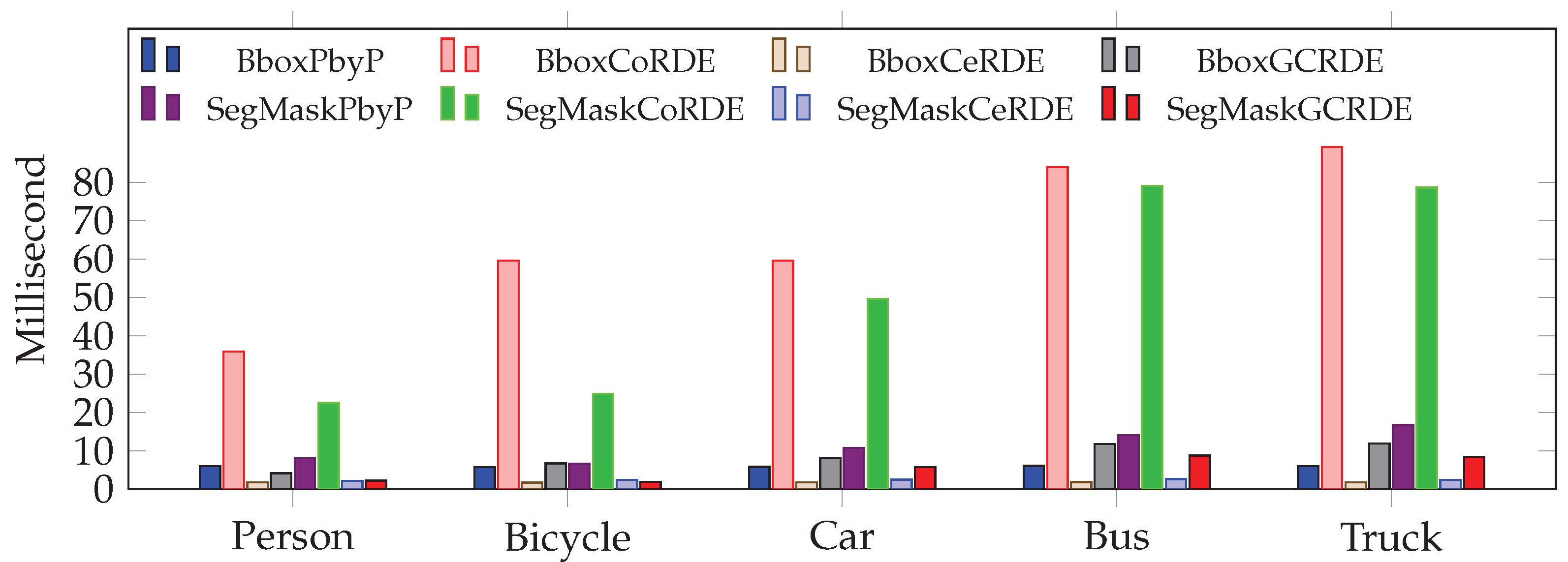
5.3. Comparative Analysis of Difficult-to-See Objects

The proposed segmentation mask in the CeRDE and GCRDE approaches provided significant improvements in processing time compared to the traditional PbyP and CoRDE approaches, as shown in Figure 26. Among all approaches, the bounding box in CeRDE achieves the lowest extraction time, particularly for the person and bicycle classes, demonstrating its high computational efficiency. In contrast, the bounding box and the segmentation mask in CoRDE exhibit the highest time consumption, making them less suitable for real-time applications.

Figure 26. This comparison shows mean depth extraction time (in milliseconds) at occlusion Levels 2 for the traditional approach: PbyP (Point-by-Point) and our proposed approaches: CoRDE (Complete Region Depth Extraction), CeRDE (Central Region Depth Extraction), and GCRDE (Grid Central Region Depth Extraction).

Figure 26. This comparison shows mean depth extraction time (in milliseconds) at occlusion Levels 2 for the traditional approach: PbyP (Point-by-Point) and our proposed approaches: CoRDE (Complete Region Depth Extraction), CeRDE (Central Region Depth Extraction), and GCRDE (Grid Central Region Depth Extraction).

The PbyP and CoRDE approaches generally yield lower accuracy, especially for the car and truck categories, as shown in Figure 27. The proposed segmentation mask in the GCRDE method achieves the highest accuracy across a lot of classes, reaching over 90% for the person class and significantly outperforming others in the truck and car categories. Also, the segmentation mask in CeRDE shows strong performance, particularly for cars and trucks.

Figure 27. This comparison shows depth extraction accuracy (%) at occlusion Levels 2 for the traditional approach: PbyP (Point-by-Point) and our proposed approaches: CoRDE (Complete Region Depth Extraction), CeRDE (Central Region Depth Extraction), and GCRDE (Grid Central Region Depth Extraction).

Figure 27. This comparison shows depth extraction accuracy (%) at occlusion Levels 2 for the traditional approach: PbyP (Point-by-Point) and our proposed approaches: CoRDE (Complete Region Depth Extraction), CeRDE (Central Region Depth Extraction), and GCRDE (Grid Central Region Depth Extraction).

The segmentation mask in the GCRDE approach achieves the lowest RMSE for trucks and persons, as shown in Figure 28. The segmentation mask and the bounding box in CeRDE also demonstrate improved depth precision compared to other approaches. PbyP and CoRDE exhibit the highest RMSE, particularly for larger objects such as buses and trucks, suggesting poor reliability in occlusion-heavy scenarios.

The bounding box and segmentation mask in the CeRDE approach outperform others in all three metrics, achieving the fastest processing time, the highest depth extraction accuracy, and the lowest RMSE. Central region depth extraction strategies provide substantial advantages over traditional approaches, especially when applied to segmentation mask objects.

Figure 28. This comparison shows depth extraction RMSE (in meters) at occlusion Levels 2 for the traditional approach: PbyP (Point-by-Point) and our proposed approaches: CoRDE (Complete Region Depth Extraction), CeRDE (Central Region Depth Extraction), and GCRDE (Grid Central Region Depth Extraction).

Figure 28. This comparison shows depth extraction RMSE (in meters) at occlusion Levels 2 for the traditional approach: PbyP (Point-by-Point) and our proposed approaches: CoRDE (Complete Region Depth Extraction), CeRDE (Central Region Depth Extraction), and GCRDE (Grid Central Region Depth Extraction).

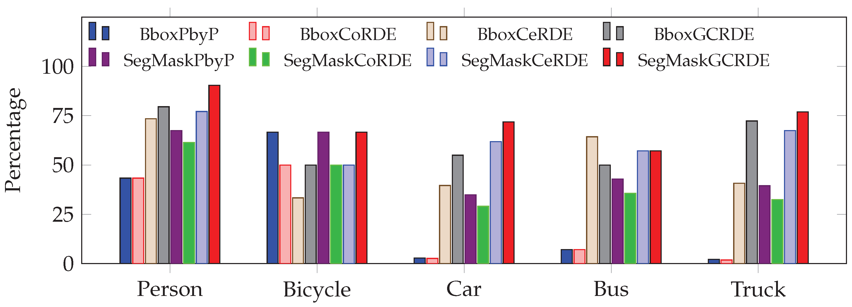
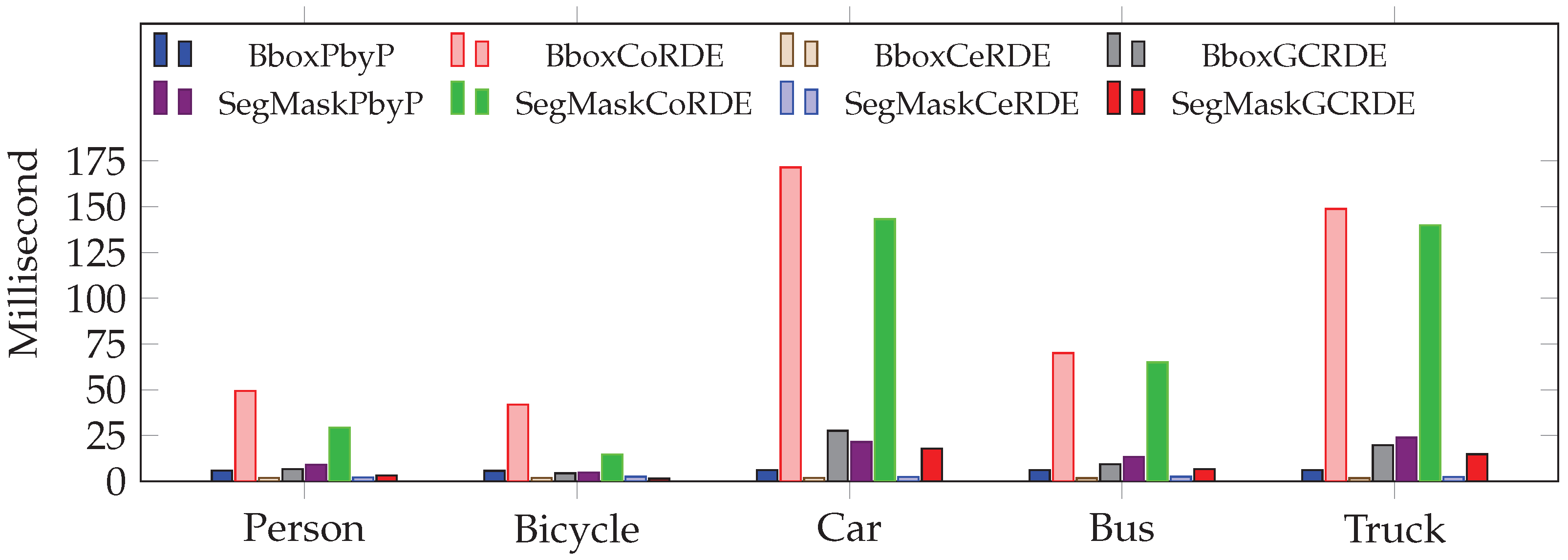
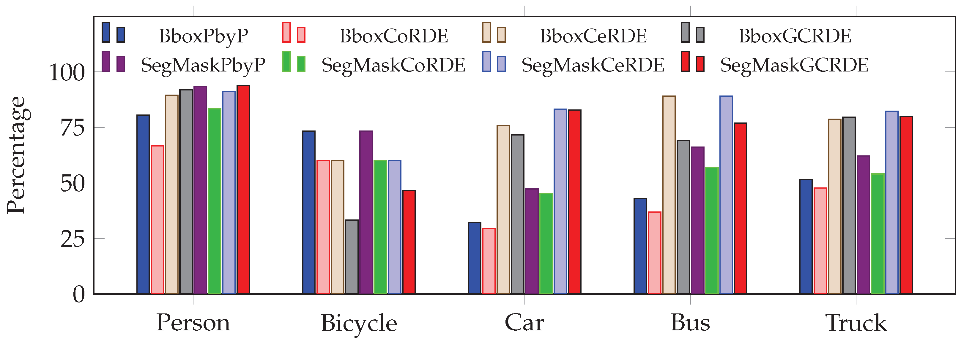
5.4. Comparative Analysis of Unknown Objects

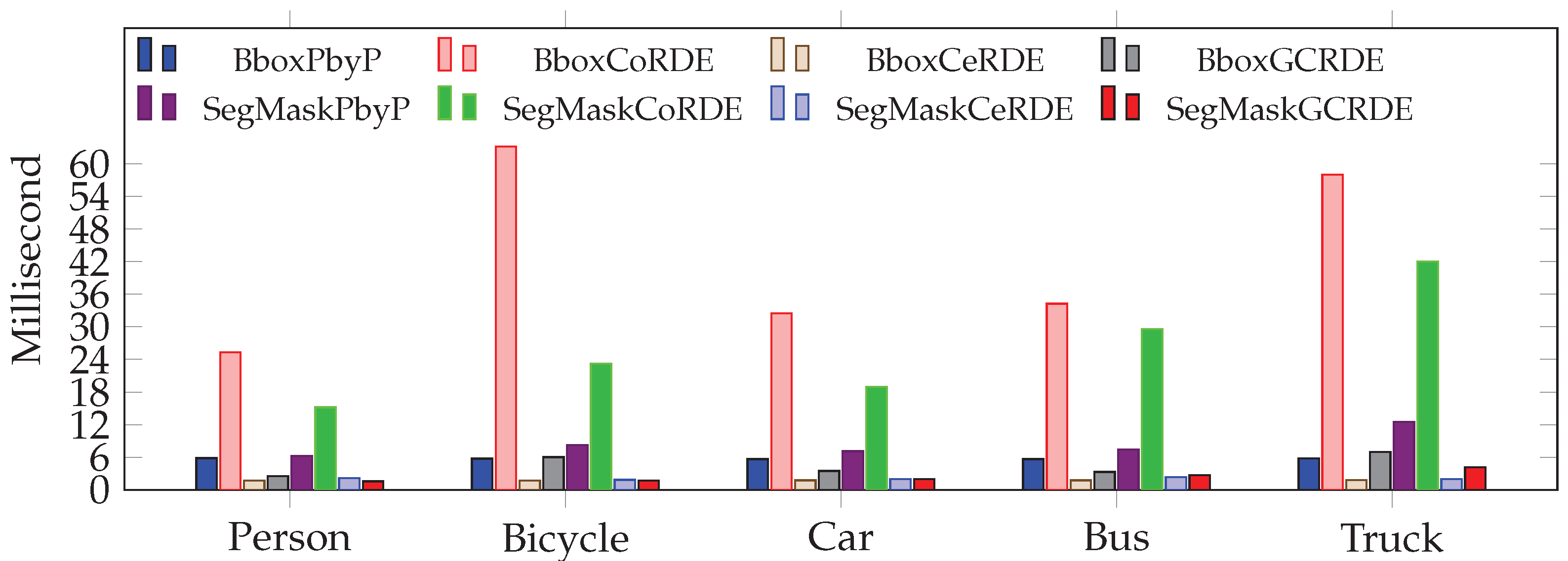
The CeRDE approach has the fastest performance, with values for the five objects ranging from 1.735 ms (truck) to 1.807 ms (bicycle), as shown in Figure 29. In comparison, the PbyP and proposed CoRDE approaches take considerably longer. GCRDE proposed another approach, showing moderate times with values from 4.43 ms (bicycle) to 27.64 ms (car). In summary, the CeRDE approach is significantly faster compared to the proposed approaches.

Figure 29. This comparison shows mean depth extraction time (in milliseconds) at occlusion Levels 3 for the traditional approach: PbyP (Point-by-Point) and our proposed approaches: CoRDE (Complete Region Depth Extraction), CeRDE (Central Region Depth Extraction), and GCRDE (Grid Central Region Depth Extraction).

Figure 29. This comparison shows mean depth extraction time (in milliseconds) at occlusion Levels 3 for the traditional approach: PbyP (Point-by-Point) and our proposed approaches: CoRDE (Complete Region Depth Extraction), CeRDE (Central Region Depth Extraction), and GCRDE (Grid Central Region Depth Extraction).

PbyP offers varying levels of accuracy across objects, with the highest accuracy for person (96.59%) and the lowest for truck (2.21%), as shown in Figure 30. The accuracy of CoRDE is generally lower than that of PbyP, with its highest accuracy for person (88.83%) and the lowest for Truck (1.85%). On the other hand, CeRDE achieves impressive accuracy for person (93.88%) and car (93.97%), making it a more accurate method overall, especially for specific objects like person and car. GCRDE performs quite well, indicating that it is the best-performing method for certain cases. Overall, CeRDE and GCRDE provide higher accuracy than PbyP, but the performance varies across different objects.

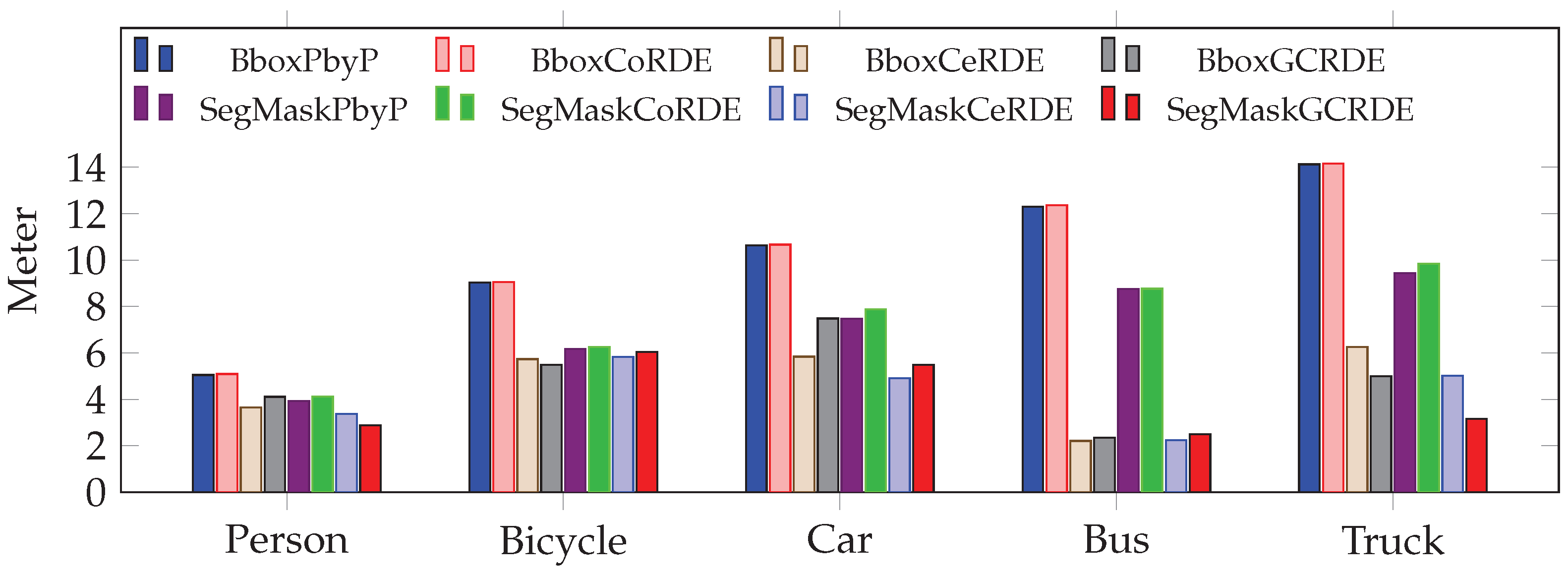
The PbyP approach shows relatively high RMSE values, ranging from 1.60 m (person) to 18.237 m (bus), which indicates less precision in depth extraction. CoRDE has worse RMSE values than other approaches, ranging from 1.785 m (person) to 18.328 m (bus). However, CeRDE shows a substantial improvement in precision, with RMSE values ranging from 1.116 m (bus) to 6.892 m (truck), highlighting its superior performance in terms of depth accuracy. GCRDE, with RMSE values ranging from 1.392 m (bus) to 7.481 (car), also offers lower RMSE than PbyP and CoRDE, making it a promising approach for better depth precision. CeRDE emerges as the most precise method in this analysis, particularly for objects, where its RMSE is significantly lower than other methods, as shown in Figure 31.

Figure 30. This comparison shows depth extraction accuracy (%) at occlusion Levels 3 for the traditional approach: PbyP (Point-by-Point) and our proposed approaches: CoRDE (Complete Region Depth Extraction), CeRDE (Central Region Depth Extraction), and GCRDE (Grid Central Region Depth Extraction).

Figure 30. This comparison shows depth extraction accuracy (%) at occlusion Levels 3 for the traditional approach: PbyP (Point-by-Point) and our proposed approaches: CoRDE (Complete Region Depth Extraction), CeRDE (Central Region Depth Extraction), and GCRDE (Grid Central Region Depth Extraction).

Figure 31. This comparison shows depth extraction RMSE (in meters) at occlusion Levels 3 for the traditional approach: PbyP (Point-by-Point) and our proposed approaches: CoRDE (Complete Region Depth Extraction), CeRDE (Central Region Depth Extraction), and GCRDE (Grid Central Region Depth Extraction).

Figure 31. This comparison shows depth extraction RMSE (in meters) at occlusion Levels 3 for the traditional approach: PbyP (Point-by-Point) and our proposed approaches: CoRDE (Complete Region Depth Extraction), CeRDE (Central Region Depth Extraction), and GCRDE (Grid Central Region Depth Extraction).

In conclusion, the CeRDE approach is the fastest and offers very good accuracy and precision. The GCRDE method strikes a balance between speed, accuracy, and precision, offering moderate performance across all three aspects. The PbyP method, while faster and more accurate than CoRDE, does not consistently outperform CoRDE in terms of RMSE. Based on the analysis, GCRDE and CeRDE are the most promising methods for applications requiring high accuracy and precision, while CeRDE is suitable for situations where speed is the primary concern.

5.5. Comparative Visualization of Depth-Based Distances

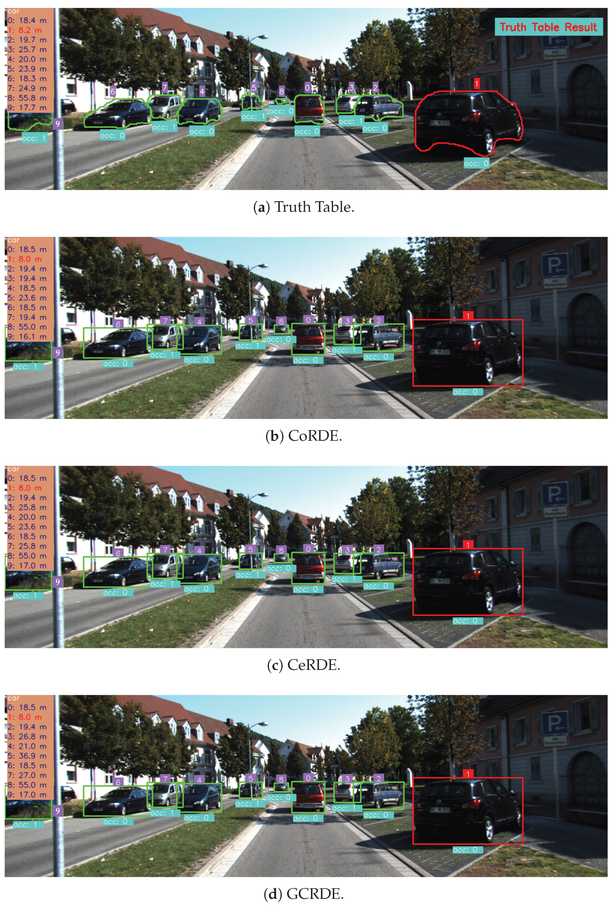
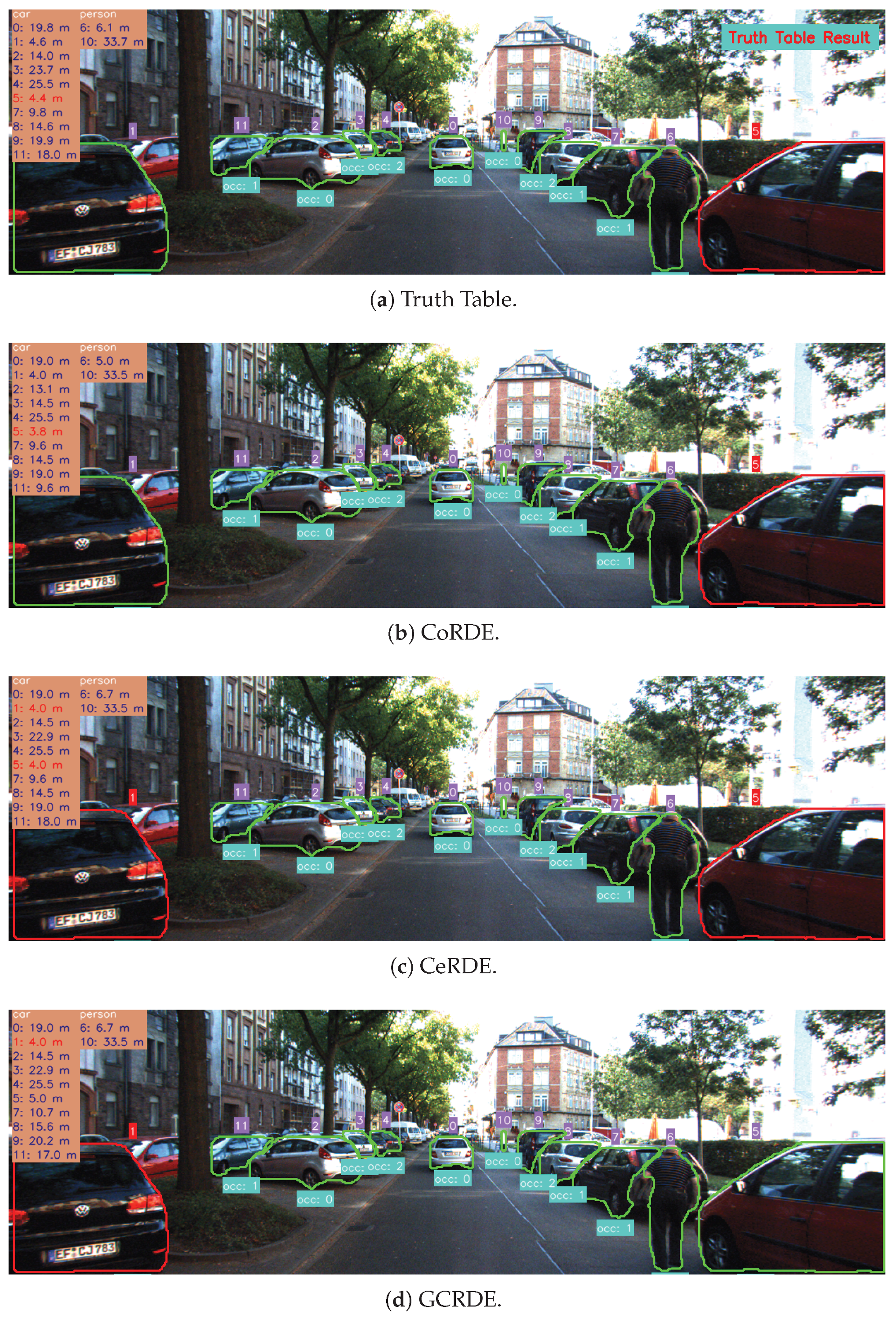
In this section, we present a comparative visualization of depth-based distance results using three extraction methods, which are CoRDE, CeRDE, and GCRDE. The figures below illustrate the output distances as interpreted through bounding boxes and segmentation masks. These visuals serve as qualitative evidence to support the numerical comparisons provided earlier. The reference truth table is included in each visualization to enable side-by-side evaluation of estimation accuracy. We analyzed various object categories, including person, bicycle, car, bus, and truck, across different occlusion levels defined as easy, medium, hard, and unknown. Additionally, the object with the closest estimated distance in each frame is highlighted with a red frame to emphasize depth prioritization.

Figure 32 presents a comparison of the transparent sparse depth map, CoRDE, CeRDE, and GCRDE across various object categories, focusing mainly on easy and medium occlusion levels, as defined by the bounding box.

Figure 32. (a) Truth Table results. (b) Complete Region Depth Extraction (CoRDE) results. (c) Central Region Depth Extraction (CeRDE) result. (d) Grid Central Region Depth Extraction (GCRDE) result. The red frame highlights the closest object.

Figure 32. (a) Truth Table results. (b) Complete Region Depth Extraction (CoRDE) results. (c) Central Region Depth Extraction (CeRDE) result. (d) Grid Central Region Depth Extraction (GCRDE) result. The red frame highlights the closest object.

Figure 33 presents a comparison of the transparent sparse depth map, CoRDE, CeRDE, and GCRDE across various object categories, with a focus on more complex, partly visible occlusion levels such as medium and hard, as defined by the bounding box. Estimating the distance for objects with partial occlusion is particularly challenging because object detection methods tend to focus on detecting the object (e.g., car, person) but often ignore obstacles in front of the object. As a result, object detection methods often detect both the object and the obstacle together. This directly affects the ability to detect the correct distance.

Figure 33. (a) Truth Table results. (b) Complete Region Depth Extraction (CoRDE) results. (c) Central Region Depth Extraction (CeRDE) result. (d) Grid Central Region Depth Extraction (GCRDE) result. The red frame highlights the closest object.

Figure 33. (a) Truth Table results. (b) Complete Region Depth Extraction (CoRDE) results. (c) Central Region Depth Extraction (CeRDE) result. (d) Grid Central Region Depth Extraction (GCRDE) result. The red frame highlights the closest object.

Figure 34 presents a comparison of the transparent sparse depth map, CoRDE, CeRDE, and GCRDE across various object categories, focusing mainly on easy and medium occlusion levels, as defined by the segmentation mask.

Figure 35 presents a comparison of the transparent sparse depth map, CoRDE, CeRDE, and GCRDE across various object categories, with a focus on more complex, partly visible occlusion levels such as medium and hard, as defined by the segmentation mask. Estimating the distance for objects with partial occlusion is particularly challenging because object detection methods tend to focus on detecting the object (e.g., car, person) but often ignore obstacles in front of the object. As a result, object detection methods often detect both the object and the obstacle together. This directly affects the ability to detect the correct distance.

6. Conclusions

In this study, we evaluated various depth extraction methods PbyP, CoRDE, CeRDE, and GCRDE across different object categories (person, bicycle, car, bus, and truck) and occlusion levels (0 to 3). The results reveal several important findings about the performance of these methods in terms of extraction time, accuracy, and RMSE.

Regarding extraction time, bounding box-based methods (PbyP and CoRDE) consistently demonstrated slower extraction times compared to segmentation mask methods (CeRDE and GCRDE). This trend was evident across all object categories. While PbyP and CoRDE took longer to extract depth, CeRDE and GCRDE were generally faster. These results indicate that GCRDE is more efficient in terms of accuracy compared to the segmentation mask methods, while CeRDE strikes a balance between speed and accuracy, making it suitable for applications requiring rapid depth extraction.

In terms of accuracy, segmentation mask-based methods, especially CeRDE and GCRDE, outperformed other approaches for most object categories and occlusion levels. Moreover, segmentation mask methods showed superior performance in more complex objects like trucks and cars, whereas bounding box methods struggled, particularly at higher occlusion levels. GCRDE with segmentation masks achieved the highest accuracy in the person, bicycle, car, and truck categories, even at higher occlusions. This suggests that segmentation masks are more effective for precise depth estimation, providing higher accuracy despite extracting fewer depth points.

RMSE analysis further supports the superior accuracy of segmentation mask methods. Both CeRDE and GCRDE provided lower RMSE values across object categories, indicating more precise depth estimations. In particular, for larger objects like trucks and buses, segmentation mask methods yielded significantly lower RMSE values, highlighting their ability to handle complex object shapes more effectively than bounding box methods, which showed higher RMSE values, particularly for larger or more occluded objects.

Overall, the findings highlight a trade-off between speed and accuracy. Bounding box methods (PbyP and CoRDE) are less efficient in terms of speed and may not be ideal for applications requiring fast depth extraction. However, segmentation mask methods (CeRDE and GCRDE) excel in accuracy, making them ideal for applications where precise depth estimation is crucial, even if they come with a higher computational cost.

These results suggest that the choice of method should depend on the specific requirements of the application, with CeRDE standing out as a well-rounded option that offers a strong balance of speed, accuracy, and low RMSE. Its ability to maintain high performance across various object categories and occlusion levels makes it particularly suitable for real-time applications where both computing efficiency and depth estimation precision are critical. CeRDE’s consistent results show its adaptability, making it an ideal choice for scenarios involving dynamic environments, such as autonomous driving, robotics, and ADAS systems.

Even though the proposed methods demonstrate promising results across different object categories and occlusion levels, this study has several limitations. One potential direction involves expanding the dataset to incorporate a larger quantity and variety of objects. In this study, sometimes obstacles such as trees, utility poles, motorcycles, and traffic cones block in front of annotated objects. These obstacles are not detected by the object detection method and are instead grouped with the target object. This causes instability and inaccurate depth estimates in applications. Moreover, in real-world challenges, adverse weather (rain, snow, fog), nighttime driving, and sensor misalignment due to mechanical vibration or calibration drift present additional limitations not yet fully addressed. These conditions may cause significant noise in the LiDAR point cloud data and reduce the effectiveness of camera-based detection. Furthermore, another limitation of our method is that the projected transparent sparse depth map encodes limited depth values, where the 0-pixel code represents 0 m, and the 255-pixel code represents 255 m. This design does not allow for the precise representation of intermediate depth values (such as 0.5 m and 10.5 m), which may increase distance accuracy in certain cases. Future work will focus on resolving these challenges by using different weather-augmented or simulated training data and self-calibrating sensor fusion frameworks to ensure robustness under failure conditions.

In addition, future research could explore advanced deep learning techniques to push the limits of sensor fusion. Transformer-based sensor fusion architectures, such as cross-attention for image-LiDAR alignment, offer a promising direction for more effective multi-modal integration. Moreover, incorporating self-supervised learning methods for depth completion can reduce reliance on annotated visual data. Multi-scale graph-based fusion approaches may also offer improvements in spatial reasoning and scene understanding. Finally, extensive evaluations in varied and complex real-world situations, including rural roads, low light, night and darkness conditions, and inclement weather, such as rainy, cloudy, snowy, and foggy conditions, will be essential to confirm the generalizability and robustness of the suggested approaches.