Real-Time Tracking and Position Control of an Elastic Cable-Driven Winch System

Abstract

This study explores the sliding mode control (SMC) strategy to address challenges such as nonlinear dynamics, steady-state errors, and torque fluctuations in elastic cable-driven winch systems. While traditional Proportional-Derivative (PD) control is sufficient for linear systems, it struggles with instability and accuracy issues in flexible systems. SMC provides robustness against uncertainties but can cause mechanical wear and performance degradation due to its chattering effect. To mitigate this, a continuous control signal-based SMC approach was adopted, reducing chattering and improving system stability. This study focuses on tracking and position control, as well as managing motor torque fluctuations during position control, emphasizing controller parameter optimization. Experimental results demonstrate that SMC outperforms PD control in tracking, position control, and torque management.

1. Introduction

Crane systems are used in various industries, including transportation and construction, and are specifically made to make handling large weights easier. These systems use high-strength structural elements and rigid cables (ropes) since they are made to support heavy loads. This ensures a safe operational process by decreasing adverse effects such as vibrations and deformations [1]. However, the limited performance of rigid cable systems in responding to sudden impacts, dynamic load variations, and complex motion paths has made it necessary to develop and find alternative solutions [2]. In this context, elastic cable winch systems have been designed to address the lack of traditional rigid cable systems. Elastic cables enhance adaptability to dynamic loads, sudden movements, and environmental factors. Their energy absorption capacity significantly improves system stability during sudden load changes and prevents failures caused by excessive stress [3]. The advantages of elastic cable systems, such as low inertia, large working area, high speed, and acceleration, provide a competitive edge over rigid arm systems, particularly in cable-operated robotic systems [4,5]. However, challenges such as tension control, sagging due to flexibility, and the complexity of control algorithms make control problems more prominent in these systems [4,5].

Various studies have been conducted on crane systems’ horizontal and vertical movements. Most researchers have focused on controlling horizontal oscillations in rotating cranes through horizontal movement [6,7,8]. Studies have typically been conducted on vertical movement on elevator systems [9] and offshore crane systems [10]. In these studies, the rope is often assumed to be non-extensible. Research on elevator systems has focused on longitudinal vibrations, and the equations of motion have been derived using Hamilton’s principle and subsequently converted into ordinary differential equations through the Galerkin method. Methods such as Lyapunov control have dissipated vibrational energy in these models [11]. Moon et al. [12] demonstrated that the rope parameters, such as time-varying stiffness, damping constant, and rope mass, evolve. Therefore, measuring the load position is crucial for load position control during vertical movements. Furthermore, N.B. Le et al. developed a simple mathematical model for a nonlinear elastic cable winch system. They applied input–output feedback linearization theory to control winch movement without requiring load position information [13].

The sliding mode control (SMC) method has emerged as a preferred control strategy for such nonlinear systems due to its robustness against varying parameters and external disturbances [14]. To mitigate the phenomenon known as “chattering,” which manifests as high-frequency oscillations in the control signal, the Equivalent Sliding Mode Control (ESMC) method has been employed, ensuring system stability against external effects [15,16,17]. For instance, the dynamics of nonlinear plants have been analyzed using ESMC, demonstrating simplified stability proofs [18]. Additionally, integrating SMC with the equivalent input disturbance approach has enhanced disturbance rejection capabilities in Stewart platform control systems [19]. In the study conducted by Wang et al., the Global Equivalent Sliding Mode Control (GESMC) method was shown through simulations to provide faster and more stable performance with less chattering compared to conventional sliding mode control (SMC) and PID control in bridge crane systems [20]. Similarly, Zhang et al. applied a Disturbance Evaluating Sliding Mode Control (DESMC) method to a four-degree-of-freedom tower crane system, incorporating the beneficial aspects of disturbance effects into the control design, thereby achieving superior control performance as demonstrated in simulations [21]. In this context, the present study advances beyond the simulation studies in [20,21] by analyzing the real-time performance of SMC approaches. The study by Xia and Ouyang implemented a super-twisting algorithm-based SMC approach in tower cranes, achieving vibration suppression and precise control while offering high robustness against external disturbances [22]. Likewise, Li et al. designed a variable structure sliding mode controller for bridge cranes to suppress load oscillations and achieve precise positioning, effectively reducing chattering in the control input [23]. Furthermore, the work by Kui et al. introduced a hybrid integral sliding mode control scheme for cable-driven parallel robots, improving tracking accuracy and mitigating vibration issues [24]. Recent studies have also suggested fixed-time controllers, which guarantee convergence within a specified time regardless of initial conditions, despite the robustness and finite-time convergence characteristics of sliding mode controllers [25,26]. These methods may be very promising for this work’s future development. The present study applies the SMC method to elastic cable winch systems to enhance tracking and position control performance.

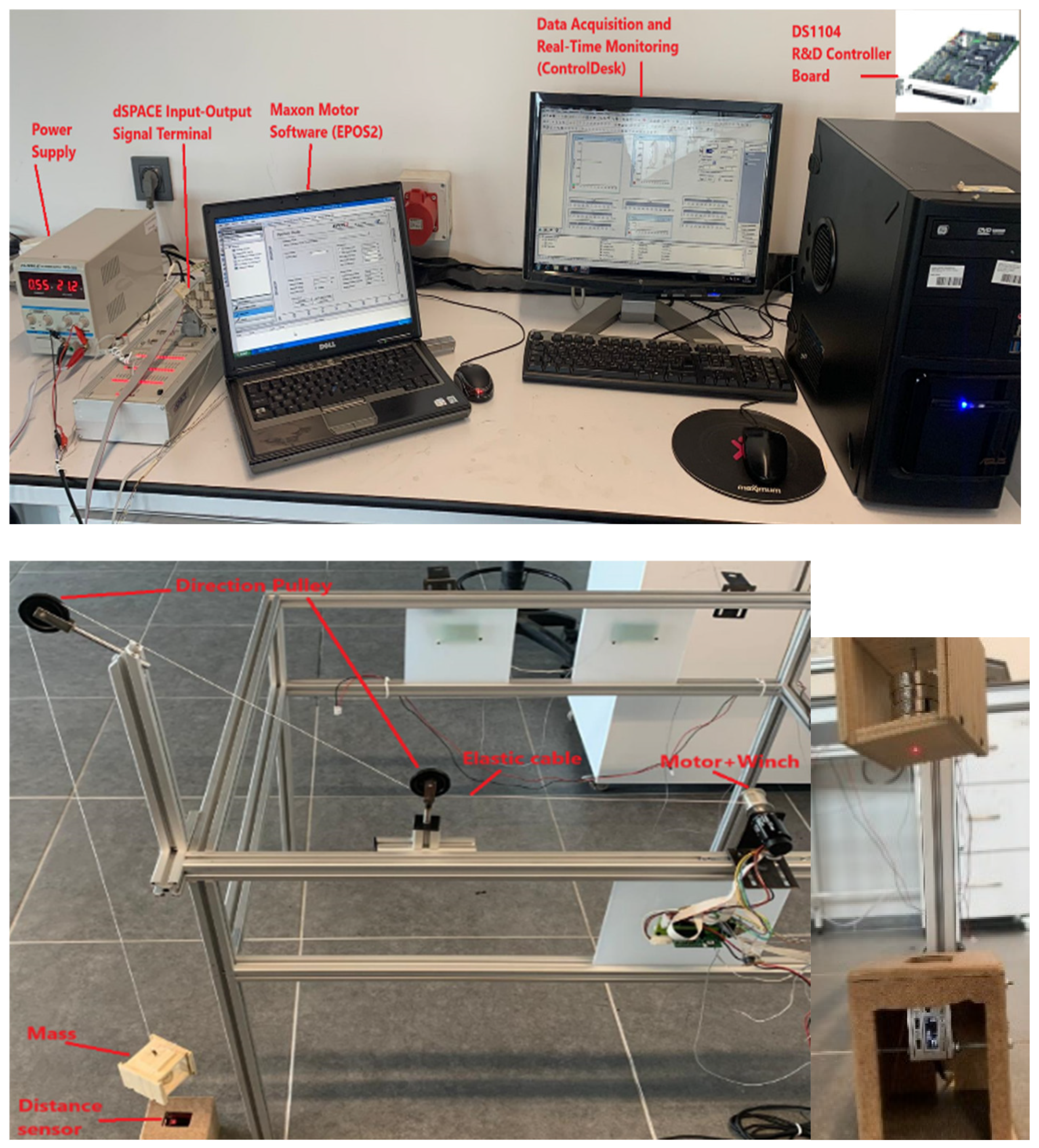
Control engineering studies aim to find practical methods to solve problems. Electromechanical systems, in particular, involve numerous uncertainties, unknown parameters, and disturbances during operation. Thus, all these factors must be considered in controlling design. In this applied engineering field, experimental studies are more convincing than pure simulation analyses. Fortunately, today’s technological advances offer experimental methods such as hardware-in-the-loop simulation or animation for real-time testing and analysis of a controller. Real-time control systems play a critical role in experimental studies. For example, using dSPACE, various control methods have been implemented in real time, verifying the performance of artificial intelligence-based asynchronous motor drives [27]. In this context, the opportunities provided by real-time control systems not only enhance the reliability of experimental studies but also optimize design processes, significantly contributing to the field of control engineering.

The contribution of this study to the literature stands out in two main aspects. First, a realistic model with four degrees of freedom was developed by considering the elastic cable stretching between the winch drum and the guide pulleys and in the vertical direction. Second, through the real-time implementation of the developed controller, the SMC controller has demonstrated superior performance with ESMC compared to the PD method. This paper presents the mathematical modeling, control design, simulation, and experimental results of an elastic cable winch system. An experimental setup was designed on a smaller scale compared to actual crane mechanisms. While cable deformations are typically negligible in real-world applications due to high load-to-cable weight ratios, this study specifically aims to examine in detail the effects of system elasticity on control performance using elastic polyester cables and light loads. This approach will make significant contributions to developing control strategies for innovative applications requiring multiple elastic cables, such as mobile compact winch systems and unmanned aerial vehicle payload transport.

The remainder of the paper is structured as follows: Section 2 presents the detailed mathematical modeling of an elastic cable crane system. Section 3 discusses the design principles and analysis of the SMC controller developed for the system. Section 4 covers the results of the experimental study and their discussion. Finally, Section 5 provides an overall evaluation of the study and offers recommendations for future research.

2. Mathematical Model of an Elastic Cable Winch System

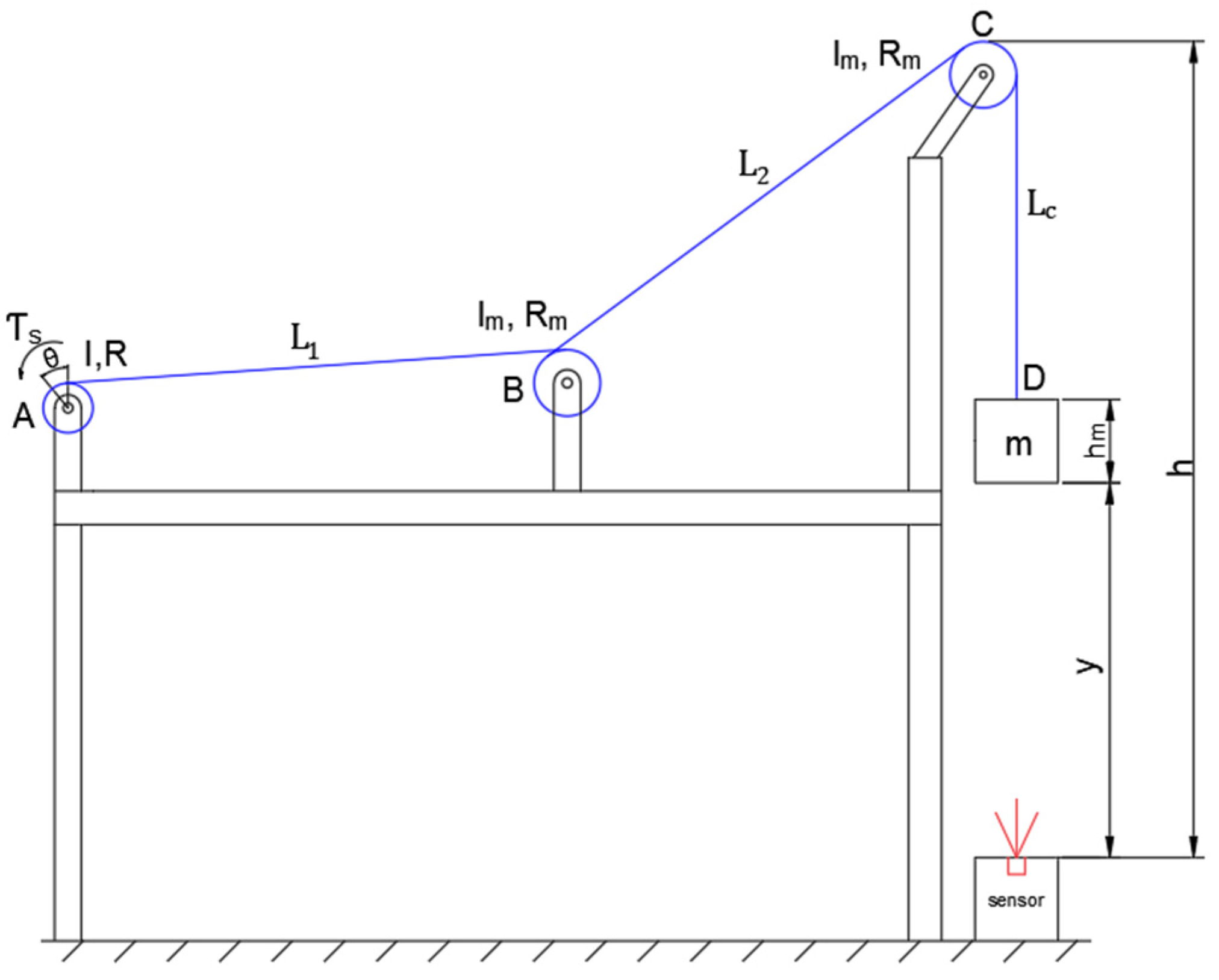
As illustrated in Figure 1, a seemingly simple system consisting of a motor and a mass is modeled more realistically by incorporating the cable’s elasticity.

For mathematical modeling of the winch system, the definition of the system is as follows: the radius of the drum and the direction pulleys are defined as R and R_m, and the moments of inertia are defined as I and I_m, respectively. The cable is determined to be homogeneous and elastic, and its mass is mc. The load consists of the combined mass of the carrier box and any additional weights. The system is structured so that the load moves vertically with the change in cable length.

The angular velocity and acceleration of the drum are demonstrated by $\dot{\theta }$ and $\ddot{\theta }$, respectively. A cable system where the segment between points A and B has a length denoted by $L_1$ and stiffness $k_1$, while the segment between points B and C has a $L_2$ length with $k_2$ stiffness. These stiffness parameters are defined as follows: $k_1=EA/L_1$, $k_2=EA/L_2$.

E represents the Young’s modulus and A is the cross-sectional area of the cable.

Assuming no slippage occurs between the cable and the pulleys, one full turn of the cable is wrapped around the directional pulleys located at points B and C. Due to the elasticity of the cable segments, the rotation angles of the pulleys at points B and C will not necessarily be identical, even if the pulleys share the same diameter. This characteristic introduces additional degrees of freedom to the system.

In this revised configuration, the system exhibits four degrees of freedom: the rotational motions of the pulleys at points A, B, and C, denoted by ${\theta }_A$, ${\theta }_B$, and ${\theta }_C$, and the vertical translation of the attached mass, represented by $y$.

The linear velocities of the cable at these points can be expressed as follows: $V_A=R{\dot{\theta }}_A,$ $V_B=R_m{\dot{\theta }}_B$, $V_C=R_m{\dot{\theta }}_C$ where $R$ and $R_m$ denote the radii of the respective pulleys, and the overdot indicates the time derivative.

$$T_A={\displaystyle \frac{1}{2}}I{\dot{\theta }}_A^2, T_B={\displaystyle \frac{1}{2}}{I}_m{\dot{\theta }}_B^2, T_C={\displaystyle \frac{1}{2}}{I}_m{\dot{\theta }}_C^2, T_y={\displaystyle \frac{1}{2}}m{\dot{y}}^2$$

To calculate the kinetic energy of the unwound portion of the cable, it is essential to determine the linear velocity of its center of mass. The length of the unwound segment is given by $L_c=h-(y+h_m)$, with mass $m_{c,CD}$, and the distance of its center of mass from the sensor is $y_c=y+h_m+0.5\ast l_c=0.5(y+h_m+h)$.

The velocity of the center of mass is thus ${\dot{y}}_c=0.5\dot{y}$.

Accordingly, the kinetic energy of this segment is approximately $T_{CD}\cong {\displaystyle \frac{1}{2}}{m}_{c,CD}{\dot{y}}_k^2$.

The linear velocity of the center of mass of the AB cable can be considered the average of these (${\displaystyle \frac{\left(V_A+V_B\right)}{2}}$). Thus, the kinetic energy of the AB segment is approximately $T_{AB}\cong {\displaystyle \frac{1}{2}}{m}_{L1}{\displaystyle \frac{{\left(V_A+V_B\right)}^2}{2^2}}$.

The total kinetic energy of the system is as follows:

$$T=T_A+T_B+T_C+T_y+T_{AB}+T_{BC}+T_{CD}$$

(1)

$$T={\displaystyle \frac{1}{2}}I{{\dot{\theta }}_A}^2+{\displaystyle \frac{1}{2}}{I}_m{{\dot{\theta }}_B}^2+{\displaystyle \frac{1}{2}}{I}_m{{\dot{\theta }}_C}^2+{\displaystyle \frac{1}{2}}m{\dot{y}}^2+{\displaystyle \frac{1}{8}}{m}_{L1}{\left(R{\dot{\theta }}_A+R_m{\dot{\theta }}_B\right)}^2+{\displaystyle \frac{1}{8}}{m}_{L2}{{R_m}^2\left({\dot{\theta }}_C+{\dot{\theta }}_B\right)}^2+{\displaystyle \frac{1}{8}}{m}_{c,CD}{{(R}_m{\dot{\theta }}_c+\dot{y})}^2$$

(2)

In this formula, $m_{L1}={\lambda L}_1$ and $m_{L2}={\lambda L}_2$ are constants and $m_{c,CD}=\lambda \left[h-\left(y+h_m\right)\right]$ is variable. The difference in the translations at the ends of the AB cable is ${∆}_1=R{\theta }_A-R_m{\theta }_B$ and the potential energy of this part is $U_{AB}={\displaystyle \frac{1}{2}}{k}_1{∆}_1^2$, for the BC cable ${∆}_2=R_m{\theta }_B-R{\theta }_C$ and $U_{BC}={\displaystyle \frac{1}{2}}{k}_2{∆}_2^2$, and for the CD cable ${∆}_3=R{\theta }_C-y$ and $U_{CD}={\displaystyle \frac{1}{2}}{k}_3{∆}_3^2$ where $k_3={\displaystyle \frac{EA}{L_C}}={\displaystyle \frac{EA}{h-(y+h_m)}}$.

The potential energy of the CD part of the cable is $U_{mc}=m_{c,CD}g{\displaystyle \frac{\left(y+h_m+h\right)}{2}}$.

The total potential energy is

$$U=U_{AB}+U_{BC}+U_{CD}+U_m+U_{mc}$$

(3)

$$U={\displaystyle \frac{1}{2}}{k}_1{∆}_1^2+{\displaystyle \frac{1}{2}}{k}_2{∆}_2^2+{\displaystyle \frac{1}{2}}{k}_3{∆}_3^2+mg\left(y+0.5h_m\right)+m_{c, CD}g{\displaystyle \frac{\left(y+h_m+h\right)}{2}}$$

(4)

The motion equations of the crane system are derived using Lagrangian mechanics. The Lagrangian function of the system is defined as the difference between the kinetic energy T and the potential energy U:

$$L=T-U$$

(5)

The equations of motion of the system are derived using the Lagrange equation.

$${\displaystyle \frac{d}{dt}}\left[{\displaystyle \frac{\partial L}{\partial {\dot{q}}_i}}\right]-{\displaystyle \frac{\partial L}{\partial q_i}}=Q_i$$

(6)

The generalized coordinates are $q_1={\theta }_A$, $q_2={\theta }_B$, $q_3={\theta }_C$ and $q_4=y,$ resulting in a total of four equations of motion.

$$\begin{array}{c}{\ddot{\theta }}_A\left(I+{\displaystyle \frac{1}{4}}{m}_{L1}{R}^2\right)+{\ddot{\theta }}_B\left({\displaystyle \frac{1}{4}}{m}_{L1}R{R}_m\right)+{{\theta }_A(k}_1{R}^2)+{{\theta }_B(-k_{1}RR}_m)=\tau \\ {\ddot{\theta }}_A\left({\displaystyle \frac{1}{4}}{m}_{L1}R{R}_m\right)+{\ddot{\theta }}_B\left(I_m+{\displaystyle \frac{1}{4}}{m}_{L1}{R_m}^2+{\displaystyle \frac{1}{4}}{m}_{L2}{R_m}^2\right)+{\ddot{\theta }}_c\left({\displaystyle \frac{1}{4}}{m}_{L2}{R_m}^2\right)+\\ {\theta }_A\left(-k_{1}R{R}_m\right)+{\theta }_B\left(k_1+k_2\right){R_m}^2+{\theta }_C\left(-k_2{R_m}^2\right)=0\\ {\ddot{\theta }}_B\left({\displaystyle \frac{1}{4}}{m}_{L2}{R_m}^2\right)+{\ddot{\theta }}_c\left(I_m+{\displaystyle \frac{1}{4}}{m}_{L2}{R_m}^2+{\displaystyle \frac{1}{4}}{m}_{C,CD}{R_m}^2\right)+\ddot{y}\left({\displaystyle \frac{1}{4}}{m}_{C,CD}{R}_m\right)\\ \hspace{1em}\hspace{1em}\hspace{1em}\hspace{1em}\hspace{1em}\hspace{1em} +{\theta }_B\left({-k}_2{R_m}^2\right)+{\theta }_C\left(k_2+k_{C,CD}\right){R_m}^2-y\left(k_{C,CD}{R}_m\right)=0 \\ \ddot{y}\left(m+{\displaystyle \frac{1}{4}}{m}_{C,CD}\right)+{\ddot{\theta }}_c\left({\displaystyle \frac{1}{4}}{m}_{C,CD}{R}_m\right)+{\displaystyle \frac{1}{8}}\mathsf{\lambda }{{(R}_m{\dot{\theta }}_c+\dot{y})}^2+g\left(m+{\displaystyle \frac{m_{C,CD}}{2}}\right)\\ \hspace{1em}\hspace{1em} +{\displaystyle \frac{k_{C,CD}}{2l_{C,CD}}}{\left(R_m{\theta }_c-y\right)}^2-k_{C,CD}\left(R_m{\theta }_c-y\right)=0\end{array}$$

(7)

The system was initially modeled as a four-degree-of-freedom (4-DOF) structure to reflect its physical characteristics accurately. However, the experimental setup includes only a single motor integrated with an encoder and a laser distance sensor for measuring the vertical position of the load. Since no sensors are available to measure the angular positions of the guide pulleys, the motions of these components cannot be directly observed. As a result, the 4-DOF model contains unobservable states, limiting its practical applicability for control design. Therefore, a reduced two-degree-of-freedom (2-DOF) model, incorporating only the measurable variables (the drum angle and the vertical position of the load) has been adopted.

The elongation occurring in the cable segments between the winch drum at point A and the guide pulley at point B, as well as between the guide pulleys at points B and C, is negligible compared to the elongation observed between the pulley at point C and the load. Therefore, the stretching behavior of the cable is primarily considered over the segment between the pulley and the load. This assumption enables the derivation of a simplified mathematical model, which forms the theoretical basis for subsequent controller design and analysis.

The stretching of the cable takes place mainly between the directional pulley and the mass. For this reason, the elongation of the cable is expressed as $∆=\theta R-y$. If the initial height of the cable is denoted by $h$, its height at any given moment can be expressed as $h-y.$ The stiffness of the cable is given by $k={\displaystyle \frac{EA}{h-y}}$. Assuming both pulleys rotate equally, the relationship between the drum’s and pulley’s angular velocities is ${\dot{\theta }}_m=\dot{\theta }{\displaystyle \frac{R}{R_m}}$.

Within the framework of simplified system dynamics modeling, the original kinetic energy expression Equation (2) has been reduced to Equation (8), while the potential energy expression Equation (4) has been simplified to Equation (9), resulting in a more streamlined formulation.

$$T={\displaystyle \frac{1}{2}}\left(m+m_c\right){\dot{y}}^2+{\displaystyle \frac{1}{2}}\left(I+2I_m{\displaystyle \frac{R^2}{{R_m}^2}}\right){\dot{\theta }}^2$$

(8)

$$U={\displaystyle \frac{1}{2}}k{∆}^2+mgy+{\displaystyle \frac{m_c}{2}}g\left(y+h+h_m\right)$$

(9)

In this system, there are two generalized coordinates: $y\left(t\right)$, which defines the vertical position of the load, and $\theta \left(t\right)$, which defines the angular position of the drum. Thus, the generalized coordinates in Equation (7) are $q_1=\theta$ and $q_2=y$, respectively. On the other hand, the generalized force is composed of the frictional force at the direction pulleys and the driving torque.

$$Q_1=-2b{\dot{\theta }}_m+T_s$$

(10)

As a result, the equations of motion of the two-degree-of-freedom winch system with elastic cable are as follows, where nonlinear effects due to the cable elasticity are noticeable.

$$\begin{array}{c}\left(I+2I_m{\displaystyle \frac{R^2}{{R_m}^2}}\right)\ddot{\theta }+2b\dot{\theta }{\displaystyle \frac{R}{R_m}}+{\displaystyle \frac{EAR}{h-y}}\left(\theta R-y\right)=T_s \\ \left(m+m_c\right)\ddot{y}+{\displaystyle \frac{EA}{{2\left(h-y\right)}^2}}{\left(\theta R-y\right)}^2-{\displaystyle \frac{EA}{h-y}}\left(\theta R-y\right)+\left(m+{\displaystyle \frac{m_c}{2}}\right)g=0\end{array}$$

(11)

3. Controller Design

In this study, motor speed control is implemented using the PID method. In contrast, PD and sliding mode control methods are used for load position control. Figure 2 illustrates the control block diagram of this winch system.

The following electrical and mechanical equations describe the mathematical model of the DC motor used in this study:

$$V_s=V_{Ra}+V_{La}+E_{emf}$$

(12)

where $V_s$ is the supply voltage, $V_{Ra}=R_a{I}_a$, $V_{La}=L_a{\displaystyle \frac{d{I}_a}{dt}}$, $E_{emf}=K_b\stackrel{.}{{\theta }_m}$

$$T_s=T_e-J_m{\ddot{\theta }}_m-T_w-T_L$$

(13)

In Equation (11), T_e is the magnetic motor torque ($T_e=K_t{I}_a$), T_w is the frictional torque ($T_w=B{\dot{\theta }}_m$), T_L is the mechanical load torque, and T_s is the output torque. The parameters of the DC motor used are shown in

Table 1. Parameters of the components used in the winch system.

	Parameters	Value	Unit
Motor Maxon ECmax-303487	Armature resistance (Ra)	3.65	[Ω]
	Armature inductance (La)	24.3 × 10−3	[H]
	Torque constant (Kt)	0.31 × 10−3	[Nm/A]
	EMF constant (Kb)	0.02429	[Vs/rad]
Winch	Drum radius (R)	0.01	[m]
	Inertia moment (I)	2409.25 × 10−9	[kgm2]
Direction pulley	Radius (Rm)	0.022	[m]
	Inertia moment (Im)	1665.88 × 10−9	[kgm2]
Elastic Cable	Diameter (d) Length at time zero (Lo) Cable length between drum-pulley (L1) Cable length between pulleys (L2) Mass per unit (qc) Max. working height (h) Modulus of elasticity (E)	1 1.70	[mm] [m]
		0.3	[m]
		0.4	[m]
		0.0013	[kg/m]
		1.00	[m]
		3.3354 × 107	[N/m2]
Load	Carrier box weight (ma)	0.077	[kg]
	Min-max payload (mb)	0–0.200	[kg]
	The maximum total mass (M)	0.277	[kg]
Distance sensor	Sensing range	50–5000	mm
Keyence LR-TB5000C	Voltage output Sensitivity	0–10 ±1	V mm

.

3.1. PD Control Design

The commonly used PD (Proportional-Derivative) controller has been selected as the initial controller design. PD control is widely recognized for improving system stability and responsiveness.

The control signal (u) is defined as the output of the PD controller, expressed by the equation:

$$U=K_p\left(y_{ref}-y\right)+K_d\left({\dot{y}}_{ref}-\dot{y}\right)$$

(14)

3.2. Sliding Mode Control

A sliding mode control (SMC) law is derived to control the desired set point of a cable-driven winch system having nonlinear properties. Next, a sliding manifold is selected to define the relationship between state variables and prescribed dynamics. Then, the control law is designed to drive the state trajectories to the manifold and restrict them there. The controller is designed using the dynamic equation of the cable-driven system in state-space form. The state variables are chosen as

$$X={\left[x_1 x_2 x_3 x_4\right]}^T={\left[\theta \dot{\theta } y \dot{y}\right]}^T$$

(15)

With the system input as U (output of the controller) and the output as y, the system is written in the state-space form as follows:

$$\begin{array}{c}\dot{x}=A\left(x\right)+B\left(x\right)U \\ y=C\left(x\right)\end{array}$$

(16)

where $x_1$, $x_2$ are the position and the velocity of the winch, respectively. $x_3$ denotes the altitude of the mass, and $x_4$ stands for the load velocity. The elements of the matrices $A$ and $B$ are as follows

$$A\left(x\right)=\left[\begin{array}{c}{x}_2\\ \begin{array}{c}-{\displaystyle \frac{2b{x}_2}{K}}{\displaystyle \frac{R}{R_m}}-{\displaystyle \frac{EAR}{K\left(h-x_3\right)}}\left(x_{1}R-x_3\right)\\ \begin{array}{c}{x}_4\\ -{\displaystyle \frac{EA}{2L{\left(h-x_3\right)}^2}}{\left(x_{1}R-x_3\right)}^2+{\displaystyle \frac{EA}{L\left(h-x_3\right)}}\left(x_{1}R-x_3\right)\end{array}\end{array}\end{array}\right]$$

(17)

$$B\left(x\right)={\left[\begin{array}{cc}0& \begin{array}{cc}{\displaystyle \frac{\eta }{K}}& \begin{array}{cc}0& 0\end{array}\end{array}\end{array}\right]}^T$$

(18)

where $K=\left(I+2I_m{\displaystyle \frac{R^2}{{R_m}^2}}\right)$, $L=\left(m+m_c\right)$, and $\eta$ is the efficiency factor. The torque of the winch system is equal to the multiplication of $\eta$ and the control signal in voltage, i.e., $T_s=\eta U$.

$$C\left(x\right)=y$$

(19)

The sliding mode manifold can be chosen as below.

$$\sigma =Ce+\dot{e}(C>0)$$

(20)

where

$$e={x_3}^r-x_3, \dot{e}={x_4}^r-x_4$$

To ensure the stability of the error dynamics, a Lyapunov function is selected as below.

$$\begin{array}{c}V={\displaystyle \frac{1}{2}}{\sigma }^T\sigma >0\\ \dot{V}={\sigma }^T\dot{\sigma }\le 0\end{array}$$

(21)

Choosing $\dot{\sigma }=-D\sigma$ (D > 0 and positive definite constant),

$$\dot{V}={\sigma }^T\dot{\sigma }=-{\sigma }^{T}D\sigma <0$$

(22)

Canceling the term ${\sigma }^T$ on both sides of Equation (22),

$$\dot{\sigma }+D\sigma =0$$

(23)

Taking the time derivative of (22) and substituting the system equations, the following is derived:

$$\dot{\sigma }=C\dot{e}+\ddot{e}=C\dot{e}+{\dot{x}}_2^r-f-bu$$

(24)

Next, the equivalent control is calculated, which satisfies the following relationship.

$$\dot{\sigma }=0\to u=u_{eq}$$

The equivalent control is found as

$$u_{eq}={\displaystyle \frac{1}{b}}\left({\dot{x}}_2^r-f+C\dot{e}\right)$$

(25)

From (24), the following equations are obtained for $\dot{\sigma }$.

$$\begin{array}{c}\dot{\sigma }=b\left(u_{eq}-u\right)\\ b\left(u_{eq}-u\right)+D\sigma =0\end{array}$$

(26)

Discretizing (25) and (26), they are obtained as follows:

$${\displaystyle \frac{\sigma \left(k\right)-\sigma \left(k-1\right)}{T}}=b\left[u_{eq}\left(k-1\right)-u\left(k-1\right)\right]$$

(27)

$$b\left[u_{eq}\left(k\right)-u\left(k\right)\right]+D\sigma \left(k\right)=0$$

(28)

u_eq (k − 1) and u_eq (k) can be solved using (27) and (28).

$$u_{eq}\left(k-1\right)=u\left(k-1\right)+{\displaystyle \frac{\sigma \left(k\right)-\sigma \left(k-1\right)}{bT}}$$

(29)

$$u_{eq}\left(k\right)=u\left(k\right)-{\displaystyle \frac{D}{b}}\sigma \left(k\right)$$

(30)

Assuming the equivalent control is an average control, and it would not change in one period,

$$u_{eq}\left(k-1\right)=u_{eq}\left(k\right)$$

(31)

Manipulating (29) and (30), the control input for the system can be derived as follows:

$$u\left(k\right)=u\left(k-1\right)+{\displaystyle \frac{1}{bT}}\left[\sigma \left(k\right)\left(1+DT\right)-\sigma \left(k-1\right)\right]$$

(32)

4. Simulation Results

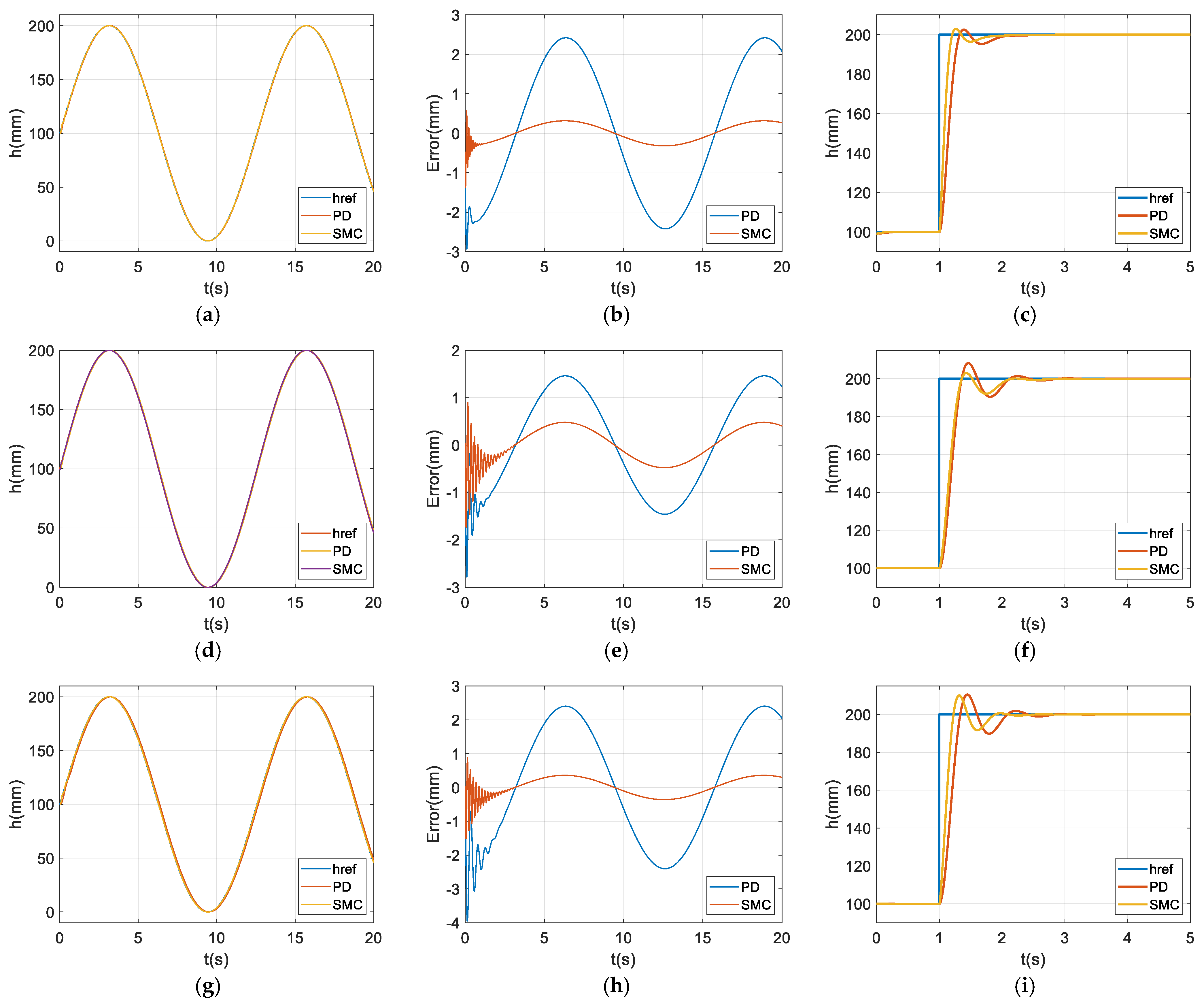
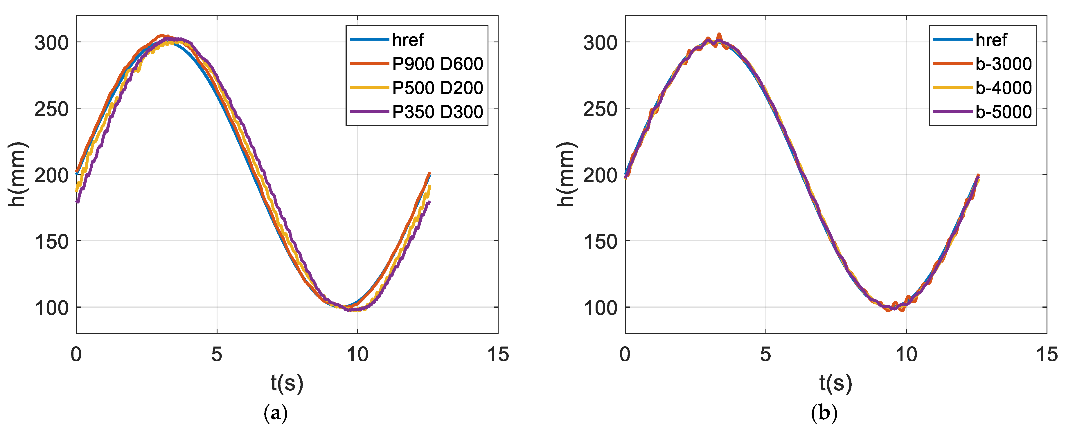
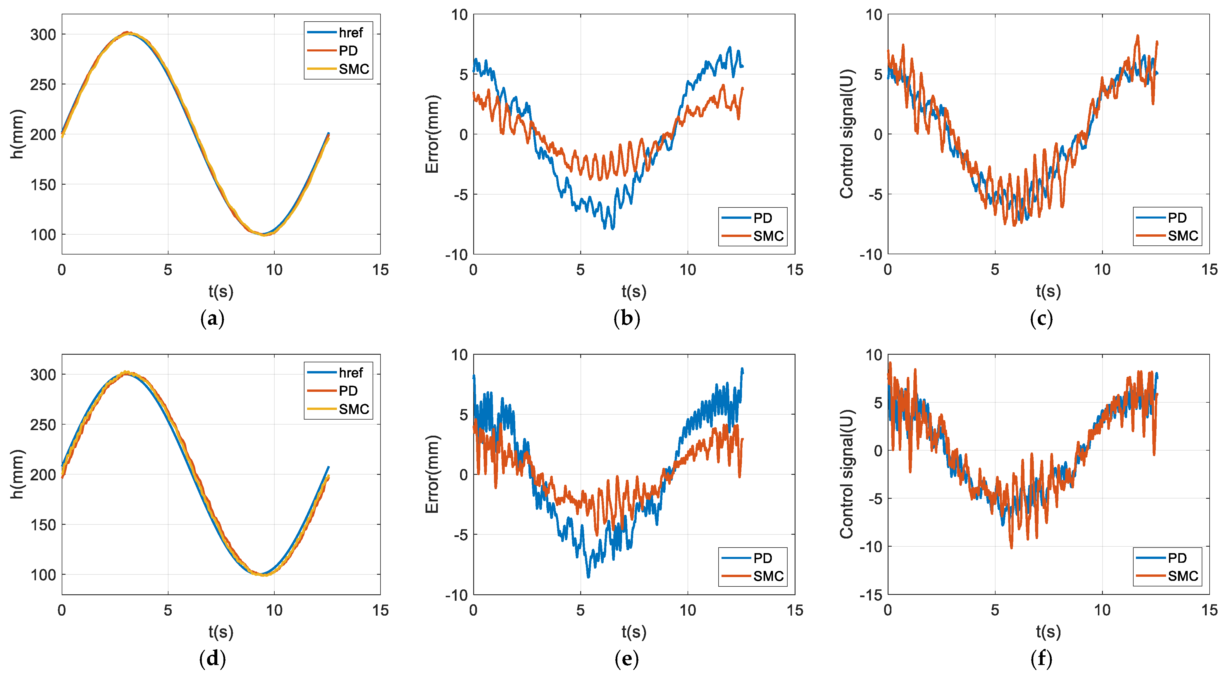
The simulation results obtained in the MATLAB/Simulink environment are presented in Figure 3. In this section, the performance of the proposed control methods is evaluated under different test cases. Test cases include the minimum, medium, and maximum load conditions shown in Figure 3.

• Subfigures (a), (d), and (g) illustrate the trajectory tracking performance;
• Subfigures (b), (e), and (h) present the tracking error between the reference trajectory and the controller output;
• Subfigures (c), (f), and (i) depict the position control performance.

In all the scenarios, the ESMC method demonstrates a more successful performance compared to PD control, withfewer errors and a faster settling time.

These simulations contributed to a better understanding of the system dynamics and enabled the validation of the control algorithms as well as a preliminary evaluation of the system behavior prior to the implementation of real-time experiments.

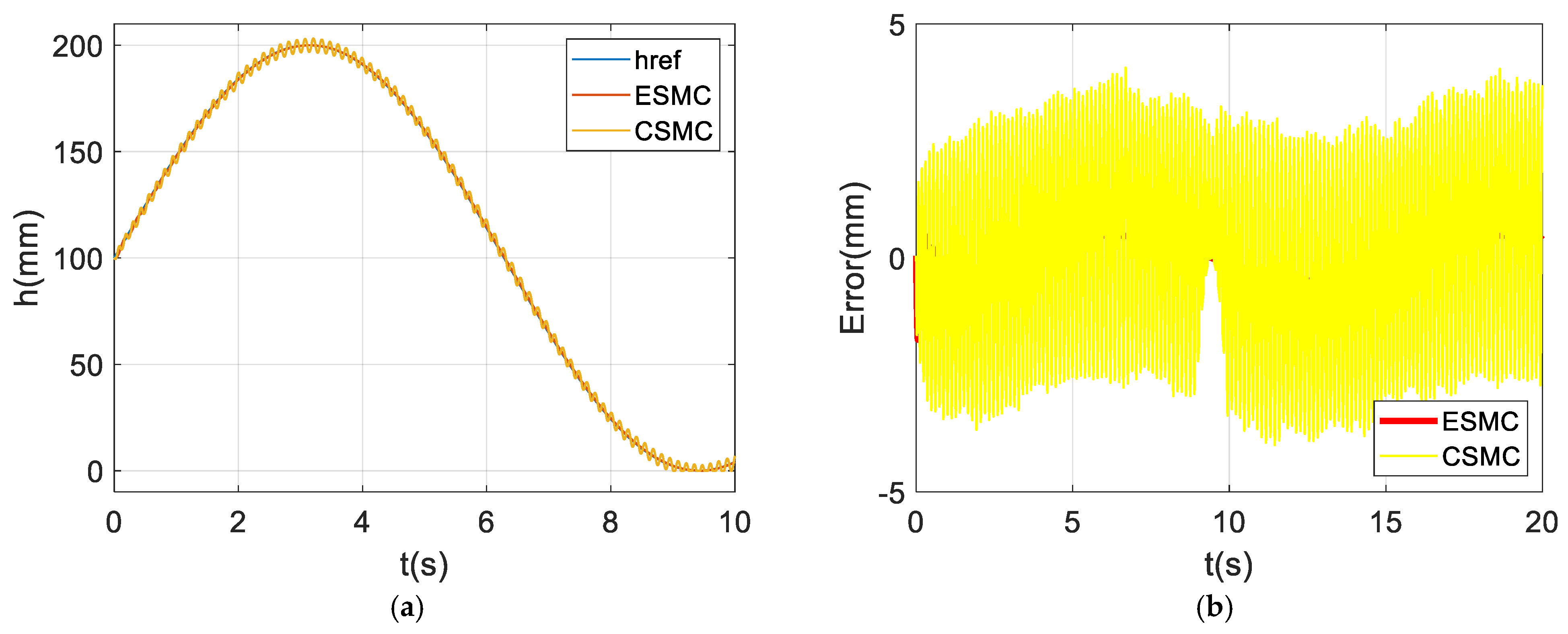
Moreover, the ESMC method and the classical SMC approach are presented in Figure 4.

In this comparison, it is observed that ESMC provides a smoother and more continuous convergence to the sliding surface. This characteristic significantly reduces the high-frequency switching (chattering) often encountered in classical SMC, thereby enhancing the system’s stability. In this respect, ESMC offers a more stable and practically applicable control structure compared to the conventional SMC. Furthermore, in the experimental studies, only the ESMC method was implemented, and the obtained results support the effectiveness of the proposed control approach.

5. Experiments

5.1. Experimental Setup

The real-time experimental setup provides a user-friendly developing environment for fast prototyping and implementing derived control algorithms. The control system is developed in the MATLAB/Simulink (R2023a) environment and executed in real time using the dSPACE DS1104 control card (dSPACE GmbH, Paderborn, Germany). The Simulink model is converted into C code and loaded onto the dSPACE card. Tests are conducted through the ControlDesk interface of dSPACE by accessing Simulink variables (Figure 5).

The position control of the winch platform was achieved by utilizing feedback from a laser distance sensor to monitor the system’s height. The parameters of the experimental winch system are given in Table 1.

5.2. Experimental Data Acquisition

Real-time parameter adjustments were made using the dSPACE ControlDesk user interface, and the process was iteratively continued until optimal results were achieved. The control method coefficients were systematically modified, and the experiments were repeated to assess the impact of these adjustments on system performance. This iterative approach identified and implemented the most effective control parameters.

The experimental results for determining the effective coefficients of the PD controller and ESMC at minimum payload condition are shown in Figure 6.

The experimental results identified the control coefficients as optimal for the system. In the PD control structure, the proportional gain (P) was set to 900 and the derivate gain (D) to 600. In the ESMC algorithm, Equation (30) was derived using a sampling time of T = 0.001 s, consistent with the DS1104 control card’s sampling period. The coefficient D was selected as 0.001, leading to the determination of the control gain b as 4000.

5.3. Experimental Results

In this study, ±100 mm sine curve reference tracking control and 100 mm position control were realized, and the maximum speed limit of the system was set to 100 rpm. To increase the controllability of the system, the speed was deliberately kept low, taking into account the effects of the long cable length. Reducing the speed made the system response more manageable and resulted in smoother operation and improved control precision.

In this section, the performance of the proposed control methods in different test scenarios is investigated. Experiments were carried out for three different loads, 0.077 kg, 0.177 kg, and 0.277 kg. The graphs presented in Figure 7 illustrate the tracking performance of the system under different payload conditions. Graphs (a), (b), and (c) correspond to Case 1 (minimum payload condition), (d), (e), and (f) represent Case 2 (medium payload condition), while (g), (h), and (i) illustrate Case 3 (maximum payload condition).

Tracking control was implemented in three different test scenarios. In all cases, examination of the tracking response and error signal graphs revealed that the SMC method provided more precise tracking performance. As shown in Figure 7g,h, with the increase in load, the PD controller struggled to maintain accurate tracking and became ineffective around the 12th second. In contrast, the SMC controller remained unaffected by the increased load and continued to provide stable and reliable control. In Figure 7c,f, the control signals are analyzed, showing that SMC produces a higher magnitude signal compared to the PD controller, which contributes to improved robustness. Additionally, Figure 7i illustrates that the PD controller had difficulty maintaining control, resulting in elevated control signal amplitudes.

As seen in Figure 8, the sum of absolute error indicates that SMC is not significantly affected by variations in load.

The performance of the position controllers lifting the load 100 mm upward is presented in Figure 9 under medium payload conditions.

An examination of the step response in Figure 9a and the positioning error in Figure 9b reveals that the SMC method provides more precise positioning compared to the PD control approach. Nevertheless, the PD controller still demonstrates an acceptable level of tracking performance. In Figure 9c, it can be observed that the control force in the SMC method is slightly increased to maintain system stability and high robustness while reducing chattering. Figure 9d illustrates the variation in acceleration ripple amplitude based on the motor’s geometric frequency, derived from the motor encoder position output to analyze the motor’s torque ripple behavior. This analysis demonstrated that the SMC algorithm systematically minimized acceleration ripple amplitude at specific frequencies (e.g., 35, 60, 85, and 115 cycles/rev). In contrast, the PD control algorithm generally maintained a higher and more constant ripple level.

6. Conclusions

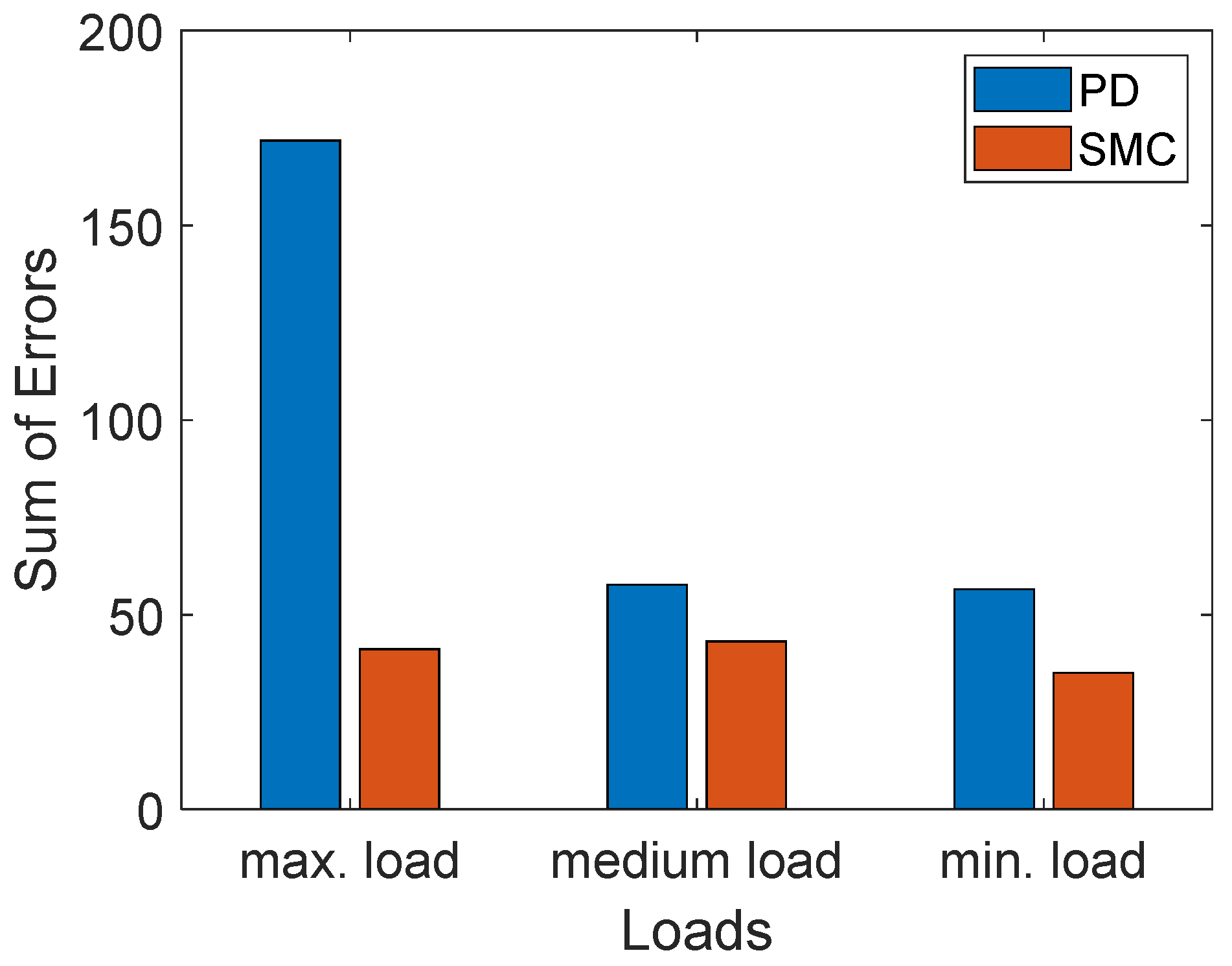
In this study, a comparative analysis of PD and SMC methods was conducted for an elastic cable-driven winch system through both simulations and real-time experiments. The simulation results demonstrated that the SMC algorithm exhibited superior positioning accuracy, reduced overshoot, and enhanced tracking performance compared to the PD controller.

Similarly, in real-time experiments, the SMC algorithm achieved higher accuracy than the PD controller in both step displacement and sinusoidal trajectory tracking tasks. Under varying load conditions, the PD controller exhibited instability at maximum load, whereas the SMC algorithm successfully maintained stable system behavior across all tested scenarios. The nonlinear structure of SMC provides increased robustness against modeling inaccuracies and parameter uncertainties, offering a significant advantage for systems operating under variable loads.

Moreover, the SMC algorithm proved more effective in minimizing torque ripple observed at the motor shaft. The analysis indicated that the SMC systematically reduced acceleration ripple amplitude at specific frequencies, while the PD controller maintained generally higher and more consistent levels of ripple.

Furthermore, during real-time experiments, only the PD controller failed to maintain control under high-load conditions, despite functioning adequately in simulation. This highlights the limitations of evaluating system performance based solely on simulations and underscores the importance of real-time testing.

Future research could concentrate on enhancing the SMC algorithm to improve motor torque ripple behavior and investigate its use in more complex systems with multiple degrees of freedom. Specifically, efforts can be focused on developing control strategies for innovative applications that involve multiple elastic cables, such as those used with unmanned aerial vehicles. Additionally, fixed-time control strategies will be compared to the sliding mode control approach used in this study, in terms of convergence time, robustness, and implementation complexity.

References

1. Zhang, C.; Hammad, A. Improving lifting motion planning and re-planning of cranes with consideration for safety and efficiency. Adv. Eng. Inform. 2012, 26, 396–410. [Google Scholar] [CrossRef]
2. He, B.; Tang, W.; Cao, J. Virtual prototyping-based multibody systems dynamics analysis of offshore crane. Int. J. Adv. Manuf. Technol. 2014, 75, 161–180. [Google Scholar] [CrossRef]
3. Michałowski, S.; Cichocki, W. The Peak Dynamic Loading of a Winch in Term of the Rope Flexibility. Key Eng. Mater. 2013, 542, 105–117. [Google Scholar] [CrossRef]
4. Zhang, Z.; Shao, Z.; You, Z.; Tang, X.; Zi, B.; Yang, G.; Gosselin, C. State-of-the-art on theories and applications of cable-driven parallel robots. Front. Mech. Eng. 2022, 17, 37. [Google Scholar] [CrossRef]
5. Gosselin, C. Cable-driven parallel mechanisms: State of the art and perspectives. Mech. Eng. Rev. 2014, 1, DSM0004. [Google Scholar] [CrossRef]
6. Ouyang, H.; Uchiyama, N.; Sano, S. Anti-sway control of rotary crane only by horizontal boom motion. In Proceedings of the 2010 IEEE International Conference on Control Applications, Yokohama, Japan, 8–10 September 2010; pp. 591–595. [Google Scholar] [CrossRef]
7. Farrage, A.; Takahashi, H.; Terauchi, K.; Sasai, S.; Sakurai, H.; Okubo, M.; Uchiyama, N. Trajectory generation of rotary cranes based on Algorithm and time-optimization for obstacle avoidance and load-sway suppression. Mechatronics 2023, 94, 103025. [Google Scholar] [CrossRef]
8. Fatehi, M.H.; Eghtesad, M.; Amjadifard, R. Modelling and Control of an Overhead Crane System with a Flexible Cable and Large Swing Angle. J. Low Freq. Noise Vib. Act. Control 2014, 33, 395–409. [Google Scholar] [CrossRef]
9. Schlemmer, M.; Agrawal, S.K. A computational approach for time-optimal planning of high-rise elevators. IEEE Trans. Control Syst. Technol. 2002, 10, 105–111. [Google Scholar] [CrossRef]
10. Johansen, T.; Fossen, T.; Sagatun, S.; Nielsen, F. Wave synchronizing crane control during water entry in offshore moonpool operations-experimental results. IEEE J. Ocean. Eng. 2003, 28, 720–728. [Google Scholar] [CrossRef]
11. Bao, J.H.; Zhang, P.; Zhu, C.M. Modeling of Rope Longitudinal Vibration on Flexible Hoisting System with Time-Varying Length. Appl. Mech. Mater. 2011, 130–134, 2783–2788. [Google Scholar] [CrossRef]
12. Moon, S.-M.; Huh, J.; Hong, D.; Lee, S.; Han, C.-S. Vertical motion control of building façade maintenance robot with built-in guide rail. Robot. Comput.-Integr. Manuf. 2015, 31, 11–20. [Google Scholar] [CrossRef]
13. Le, N.B.; Tran, M.S.; Jung, S.H.; Kim, Y.B. Vertical Motion Control of Crane Without Load Position Information Using Nonlinear Control Theory. In AETA 2017-Recent Advances in Electrical Engineering and Related Sciences: Theory and Application; Springer: Cham, Switzerland, 2017; pp. 405–415. [Google Scholar] [CrossRef]
14. Utkin, V. Variable structure systems with sliding modes. IEEE Trans. Autom. Control 1977, 22, 212–222. [Google Scholar] [CrossRef]
15. Bai, Y.; Roth, Z.S. Practical Nonlinear Control Systems. In Classical and Modern Controls with Microcontrollers. Advances in Industrial Control; Springer: Cham, Switzerland, 2019; pp. 323–435. [Google Scholar] [CrossRef]
16. Young, K.D.; Utkin, V.I.; Ozguner, U. A control engineer’s guide to sliding mode control. IEEE Trans. Control Syst. Technol. 1999, 7, 328–342. [Google Scholar] [CrossRef]
17. Edwards, C.; Spurgeon, S.K. Sliding Mode Control: Theory and Applications; CRC Press: Boca Raton, FL, USA, 1998. [Google Scholar]
18. Boiko, I. On plant dynamics transformation through addition of equivalent control. J. Frankl. Inst.-Eng. Appl. Math. 2024, 361, 106930. [Google Scholar] [CrossRef]
19. Mei, Q.; She, J.; Wang, F.; Wu, M.; Wang, Q.-G.; Nakanishi, Y. Performance Enhancement for an Equivalent-Input-Disturbance-Based Control System Using a Sliding-Mode Controller. IEEE-ASME Trans. Mechatron. 2023, 28, 1456–1465. [Google Scholar] [CrossRef]
20. Wang, T.; Tan, N.; Qiu, J.; Yu, Y.; Zhang, X.; Zhai, Y.; Labati, R.D.; Piuri, V.; Scotti, F. Global-Equivalent Sliding Mode Control Method for Bridge Crane. IEEE Access 2021, 9, 160372–160382. [Google Scholar] [CrossRef]
21. Zheng, H.; Li, Y. Disturbance employment-based sliding mode control for 4-DOF tower crane systems. Mech. Mach. Theory 2021, 165, 104443. [Google Scholar] [CrossRef]
22. Xia, J.; Ouyang, H. Chattering Free Sliding-Mode Controller Design for Tower Cranes. IEEE Trans. Ind. Electron. 2024, 71, 4963–4975. [Google Scholar] [CrossRef]
23. Li, X.; Shi, L.; Zhang, Y.; Ma, W.; Wu, K.; Chen, L. Sliding Mode Control of Bridge Crane. In Proceedings of the 2022 34th Chinese Control and Decision Conference (CCDC), Hefei, China, 15–17 August 2022; pp. 4221–4224. [Google Scholar] [CrossRef]
24. Kui, Q.; Li, X.; Lu, Y.; Huan, B.; Xiang, Z.; Tang, F. Hybrid Integral Sliding Mode Tracking Control of Cable-Driven Parallel Robots. In Proceedings of the 2024 IEEE 7th International Electrical and Energy Conference (CIEEC), Harbin, China, 10–12 May 2024; pp. 1608–1613. [Google Scholar] [CrossRef]
25. Polyakov, A. Nonlinear feedback design for fixed-time stabilization of linear control systems. IEEE Trans. Autom. Control 2012, 57, 2106–2110. [Google Scholar] [CrossRef]
26. Chen, C.C.; Chen, G.S. A novel approach to fixed-time stabilization for a class of uncertain second-order nonlinear systems. Appl. Sci. 2020, 10, 424. [Google Scholar] [CrossRef]
27. Menghal, P.M.; Jaya Laxmi, A. Artificial Intelligence-Based Real-Time Control of Induction Motor Using dSPACE Controller. In Advances in Automation, Signal Processing, Instrumentation, and Control; Springer: Singapore, 2021; pp. 801–815. [Google Scholar] [CrossRef]
Figure 1. A schematic elastic cable winch system.
Applsci 15 05462 g001
Figure 2. The real−time block diagram of position control and PID velocity control.
Applsci 15 05462 g002
Figure 3. Simulation results. Case 1: Min. payload (0.077 kg) (ac); Case 2: Medium payload (0.177 kg) (df); and Case 3: Max. payload (0.277 kg) (gi).
Applsci 15 05462 g003
Figure 4. Comparison of ESMC and CSMC−tracking response (a); error signal (b).
Applsci 15 05462 g004
Figure 5. Experimental setup of a real-time controlled winch system with an elastic cable.
Applsci 15 05462 g005
Figure 6. Determination of (a) the PD coefficients and (b) the ESMC coefficients.
Applsci 15 05462 g006
Figure 7. Tracking response, error signal, and control signal graphs for (ac) Case 1, (df) Case 2, and (gi) Case 3.
Applsci 15 05462 g007aApplsci 15 05462 g007b
Figure 8. The sum of absolute errors for each case.
Applsci 15 05462 g008
Figure 9. Comparison of two control methods for a 100 mm reference: position response (a), error signal (b), control signal (c) and motor’s torque ripples (d).
Applsci 15 05462 g009