Abstract
This study presents an enhancement in the prediction of aggressive outbursts in dementia patients from our previous work, by integrating audio-based violence detection into our previous visual-based aggressive body movement detections. By combining audio and visual information, we aim to further enhance the model’s capabilities and make it more suitable for real-world scenario applications. This current work utilizes an audio dataset, containing various audio segments capturing vocal expressions during aggressive and non-aggressive scenarios. Various noise-filtering techniques were performed on the audio files using Mel-frequency cepstral coefficients (MFCCs), frequency filtering, and speech prosody to extract clear information from the audio features. Furthermore, we perform a late fusion rule to merge the predictions of the two models into a unified trained meta-classifier to determine the further improvement of the model with the audio integrated into it with a higher aim for a more precise and multimodal approach in detecting and predicting aggressive outburst behavior in patients suffering from dementia. The analysis of the correlations in our multimodal approach suggests that the accuracy of the early detection models is improved, providing a novel proof of concept with the appropriate findings to advance the understanding of aggression prediction in clinical settings and offer more effective intervention tactics from caregivers.
1. Introduction
1.1. Dementia
Dementia is a condition commonly known for affecting cognitive function because of its progressive neurodegenerative characteristics. A variety of symptoms can manifest, such as aggression, which is very common and challenging through verbal and physical aggression or restlessness. Dementia can also affect memory, language, reasoning, and behavior. It can be caused by various disorders, with the most common being Alzheimer’s disease, and over time, it can impair an individual’s daily functioning. As symptoms progress over time, patients often showcase declines in communication and judgment, mood swings, and personality changes. From the symptoms mentioned above, aggression is most commonly associated with dementia and can manifest both in verbal and physical aggression episodes and agitation [1].
According to findings from studies, 50% of dementia patients exhibit at least one form of aggressive behavior, which can be harmful to caregivers and mental healthcare workers, as well as patients. Aggressive behaviors can be triggered by frustration, confusion, pain, or environmental changes. Such behaviors can pose significant risks to patients themselves and healthcare employees, in turn, increasing stress and emotional burden. Patients sometimes may harm themselves and cause injuries, episodes that increase the patient’s condition over time [2].
The early prediction of these symptoms, before their escalation, presents a significant objective because it can provide the opportunity for timely interventions that can reduce the severity of these episodes, thereby reducing distress for patients and caregivers. Timed interventions can also de-escalate high risk situations and provide time to formulate treatment plans and preventive measures, hence decreasing harm and distress while reducing pharmacological treatment. Previous research has relied heavily on visual cues to detect and predict such aggressive behaviors. By integrating audio-based feature analysis, a more robust prediction method can be provided based on multimodal analysis while increasing prediction accuracy [3].
The mini-mental state examination (MMSE) is commonly used in cognitive impairment screening, with limited effectiveness in dementia progression prediction in patients suffering from mild cognitive impairment (MCI). Researchers, in a review of 11 studies with approximately 1569 patients suffering from MCI, found that the MMSE is not accurate in predicting conversion to dementia, indicating the need for multiple longitudinal assessments [4]. In a review, researchers analyzed 52 cognitive assessment tools commonly used for the identification of mild cognitive impairment (MCI) in its early stages. This review identified the Montreal cognitive assessment (MoCA), mini-mental state examination (MMSE), and clock-drawing test (CDT) as the most cited techniques, with the six-Item cognitive impairment test (6CIT) and the Hong Kong brief cognitive test (HKBC) as the most recommended, taking into account various factors, such as age and education level [5]. Another team of researchers reviewed cognitive impairment and dementia detection in emergency departments. The final results highlight the need for more pragmatic and effective screening approaches and for improved detection techniques in dementia [6].
1.2. Dementia and Machine Learning
Clinical translations in automated dementia diagnosis using machine learning are promising; however, there is also a need for machine-learning models that can generalize well and have improved robustness. Although the research in this field is developing, there are a lot of occurrences of validation inconsistency, while reliance on common datasets improves interpretability and stability. Therefore, the needs for further clinical expertise and focus are crucial [7]. Another study showcases promising solutions for machine-learning applications in the automated prediction of dementia diagnosis. That review examines dementia diagnostic models from 2011 to 2022, with considerations of the modalities of the data. The results demonstrate exceptional performance but with a variety of limitations for future directions [8].
In the fields of medicine and dementia research, there is rapid growth in machine-learning applications that automate the predictions of diagnosis and treatment for the corresponding patients. Another study compares deep-learning models with machine-learning models, showcasing the deep-learning models’ ability to achieve higher-accuracy results compared to those of the traditional machine-learning models and indicating a need for higher computational power and resources. The problems of data scarcity and applications present an obstacle in the further development of such models, even though they show promise for application in dementia care [9].
A meta-analysis study discusses the challenges of Alzheimer’s disease (AD) diagnosis because of the limitations of the current methods in cognitive tests and imaging analysis. That study, exploring the potential of machine-learning models using novel biomarkers, highlights a new way to enhance AD diagnosis accuracy [10]. Similarly, machine learning was utilized for the early detection of dementia, with test scores in cognitive function being used as features for these predictions. The ensemble model of AdaBoost achieved a high accuracy rate of 83%, outperforming other models and showing potential use for AI in diagnoses [11]. Another research study focused on Alzheimer’s disease (AD) and frontotemporal dementia (FTD) and the serious challenges these pose for healthcare and caregivers. In that study, a new approach was proposed using deep learning and EEG classification for AD and FTD by implementing improved preprocessing classification. The results indicated a potential solution for such deep-learning implementation in dementia screening [12].
Finally, another study analyzed Alzheimer’s disease, amyotrophic lateral sclerosis (ALS), and frontotemporal dementia (FTD) and their shared molecular pathophysiology with the use of unsupervised learning. The results revealed a substantial correlation between key molecules [13].
1.3. Detection and Prediction of Episodes of Aggression in Patients with Dementia
In dementia disorders, episodes of agitation and aggression can pose significant challenges for caregivers and mental health facilities when it comes to timely interventions. In a systematic umbrella review, technologies that monitor activities and behavioral symptoms in old-age patients with neurodegenerative diseases were examined. Their application, although promising, faces many challenges because of methodological diversity and the need for standardized metrics in the development of ethical AI in healthcare [14]. The use of wearable sensors is investigated in an attempt to develop a personalized machine-learning model for behavioral and psychological symptoms of dementia (BPSD). That study focused on the development of digital biomarkers, further enhancing the approaches in the digital phenotyping of BPSD [15].
Another study introduces a public dataset, using non-intrusive sensors, such as wearables or cameras, which monitor agitation-related physical behavior in patients suffering from dementia. The findings indicated a high accuracy rate under controlled conditions, but in leave-one-out scenarios, a decline was observed, showcasing the challenges in the invariance domain [16]. Another study presents an efficient computational technique for real-time aggressive behavior detection with the use of a wrist accelerometer. This wireless actigraphic approach collects behavioral symptom data. Its effectiveness is limited, however, because of low computational power [17]. Subsequently, a machine-learning classification model, based on the MediaPipe holistic model, has been suggested and can detect and classify episodes of aggressive behavior in real-time. That proof-of-concept study presents a new approach with the potential to predict episodes of aggression, in patients with dementia, before their onset [18].
1.4. Audio Classification and Machine Learning
A classification method for sound, with the use of convolutional neural networks (CNNs) and Mel-frequency cepstral coefficients (MFCCs) for sound conversion to spectrograms suitable to be used as inputs for CNNs, has been proposed. This method improved the classification accuracy of the dataset from 63% to 97% and offered various benefits, such as faster training [19]. The diversity of acoustic quantification in vocal audio has been used in a generalizable method with an unsupervised random forest framework. The authors demonstrated that their method could classify acoustic structures with a high degree of accuracy, offering a standard tool for music variation comparison [20]. Moreover, the use of Mel spectrograms has been evaluated using the architectures of convolutional neural networks (CNNs) and long short-term memory (LSTM) networks. The findings showcase that a hybrid model, using compression techniques, Taylor pruning, and 8-bit quantization, achieved a high accuracy rate compared to those of traditional methods while using minimal computational resources [21].
A systematic review analyzed machine-learning techniques with small-data augmentation for audio-based sound classification, including voice and speech. The analysis presented common challenges, such as insufficient or highly noised data, as well as their impacts on the classification performance. That review sheds light on sound analysis for feature extraction [22]. A later survey examined multiple audio classification deep-learning models with the main focus on five architectures: convolutional neural networks (CNNs), recurrent neural networks (RNNs), autoencoders, transformers, and hybrid models. Standard audio transformation techniques, such as spectrograms and Mel-frequency cepstral coefficients (MFCCs) were included [23]. A systematic literature review of small data and augmentation techniques examined the potential for improving classification via the deep learning of sound features, while identifying challenges, such as noise or data insufficiency, which make feature extraction difficult and unreliable. Recommendations were made in this context for the enhancement of the performance of sound classification [22]. A recent study explores the repeated training of an already trained convolutional neural network to investigate the impacts on the accuracy and processing time that the retraining parameters will have across several sound datasets [24].
1.5. Machine-Learning Multimodal Approaches with Late Fusion and a Meta-Classifier
Multimodal approaches in machine learning provide a new and powerful tool to enhance the prediction capabilities of a model. A fusion-based machine-learning prediction model has addressed data imbalances by combining classifiers and resampling techniques, improving the overall accuracy rate. The fusion model achieved the highest scores in recall, accuracy, precision, and F1-scores, showcasing the potential of this fusion strategy for breast cancer diagnosis [25].
Multimodal networks that can analyze text and audio are valuable tools for the early detection of mental health disorders. Another study, proposed early and late fusion techniques in multimodal networks for early depression detection, showing highly accurate classification metrics and indicating potential for future depression detection applications [26]. Another team of researchers focused on multimodal emotional prediction with real-time data from physiological markers to automate emotional recognition while handling complexities, such as the diversity of expression methods.
Various ensemble models using real-world data were evaluated and combined with base learners. These were the non-parametric algorithm for classifying data points among the closest neighbors or k-nearest neighbors (KNNs), tree-based models that decide based on rules from data-feature decision trees (DTs), ensemble methods for enhanced classification accuracy by combining multiple decision trees or random forests (RFs), as well as supervised learning models, which find the best optimal hyperplane for classification, defined as support vector machines (SVMs). These achieved high-accuracy results [27]. Deep-learning techniques for detection in homogeneous and heterogeneous sensing scenarios were reviewed using public datasets and deep-learning models [28]. Subsequently, a novel framework was proposed that combined emotional speech recognition and emotional analysis, utilizing features and various deep-learning models. The results demonstrated the benefits of ensemble methods and the need for multimodal fusion for affective emotional analysis [29]. Another study presents a neural-network-based approach for emotional recognition through the use of a wearable stress and affect detection (WESAD) dataset, focusing on wrist-measured blood volume–pulse (BVP) and electrodermal activity (EDA) data. The Siamese model late-fusion-based method exhibited a 99% accuracy in classifying four different emotional states. The model was further optimized for hardware acceleration, adding potential real-time usage in detection systems [30]. Hybrid meta-learning models have achieved strong results in research areas considering time-series forecasting. Another study proposed a time-series-related meta-learning (TsrML) approach and utilized a meta-learner and a base learner in multiple datasets to observe fast adaptation to new small-sample data, outperforming other deep-learning models in terms of accuracy [31].
1.6. Objective
In this study, the main objective is to develop a combined machine-learning model that can precisely classify verbal aggressive and non-aggressive arguments. The model to be combined is an audio model, which uses audio clips from a vast dataset with variations in aggressive and non-aggressive speech instances.
Following audio data processing using filtering techniques, such as Mel-frequency cepstral coefficients (MFCCs) and pitch filtering [32,33], the filtered data are fed into a machine-learning model with the same methodology as its predecessor. After training and testing the model, the prediction capabilities of this model, after the final evaluation, combine the predictions of our visual-based detection model from our previous work with the audio detection results from our current model. The combination of the predictions of these two models employs the late fusion rule [26]. The fused unified predictions are being fed into a meta-classifier model [34] that will be trained on the new data, thus providing better and enhanced prediction capabilities in aggressive outbursts from dementia patients, utilizing both visual and audio information.
1.7. Novelty and Key Contributions
In this study, an enhancement to a previous novel approach is presented, which improves the accuracy and efficiency of aggressive behavior prediction in patients suffering from dementia. The integration of an audio-based detection system combined with a previously developed vision-based model can improve behavior prediction.
The main contributions of this study are as follows:
Potential Benefits from the Previous Work:
- Multimodal Aggression Detection: The introduction of a multimodal technique is presented, combining previously existing visual-based aggression analysis with a new audio-based aggression analysis, thereby enhancing the system’s robustness in real-world scenarios with improved noise reduction;
- Advanced Audio-Processing Techniques: In order to successfully extract audio features from audio files, advanced techniques of audio processing were used, such as Mel-frequency cepstral coefficients (MFCCs), frequency filtering, and speech prosody, improving the model’s classification accuracy;
- Late Fusion Meta-Classifier: A late fusion meta-classifier was applied to merge the multilayered model predictions into a unified data frame consisting of both audio and visual aggression predictions;
- Clinical Applicability and Proof of Concept: The results showcase that the multimodal framework’s implementation improves the detection of early aggression behaviors, providing proof-of-concept validity for the future support of clinical practice.
New Insights:
- The results of this multilayer approach demonstrate that when audio-based aggression predictions are merged with visual prediction, the overall aggression prediction is improved, providing a more comprehensive approach to patient behavior;
- The correlations between body movements and vocal frequencies provide insight into their association.
Practical Implications:
- This multimodal system could support real-world clinical systems by providing real-time alerts generating suitable interventions;
- Because of its enhanced accuracy, this approach could be integrated into future clinical practice.
2. Materials and Methods
Following previous research in which a machine-learning model was developed as a proof of concept to detect and predict episodes of aggressive behavior in patients with dementia [18], in this study, a second model was developed, which classifies aggressive and non-aggressive verbal communications, utilizing the Python 3.12.3 language and Python libraries, such as SciKit, OpenCV, and Pandas. The random forest classifier was selected in order to follow the same classification approach. The pipeline used during the training and the testing of the audio classification model was also identical to that used for the progenitor model. The main aim was to create a second machine-learning model based on audio features that would further enhance the performance of the previous model, with a more robust method for predicting aggressive outbursts in dementia patients. High priority was given to techniques for noise control and overfitting prevention.
2.1. Data Collection and Processing
In this study, a dataset from the Kaggle “Audio-based Violence Detection Dataset” [35] was utilized. The dataset was structured in one folder containing 131 audio .wav files. Each file had a naming convention labeled appropriately, pinpointing its class type. The number of files labeled as angry.wav was 127 in total, and each file contained from 15 s to 15 min of aggressive or violent verbal audio interactions from various daily conversations between individuals. The number of files labeled as nonviolence, which contained casual audio verbal interactions, was four in total, with each file containing approximately 1 h of audio footage. A detailed analysis of the files is shown in Table 1.

Table 1.
Demonstration of files’ data structure.
Initially, all the audio files were loaded into memory, using a library for audio analysis (Librosa). Because of the imbalanced nature of the dataset, necessary steps were followed in order to separate larger audio files into smaller chunks and process them accordingly. All the audio files were separated by code into smaller chunks, producing audio samples consisting of 15 s of audio information. The audio files that were not equally partitioned were discarded to maintain uniformity. Regarding the nonviolence audio clips, they were four in count and long in duration and were split in order to ensure an identical number of total audio files between aggression and non-aggression cases (anger and nonviolence audio files).
Because these audios were sampled from various real-world daily life interactions, the information within the audio files contained unwanted noise and artifacts. Before any further processing, in order to isolate the distortion of the information, bandpass filtering was first applied to isolate frequencies within a specific range. Audio signals were filtered in the range from 85 Hz to 255 Hz to reduce noise and focus on specific vocal ranges. Unwanted noise within this range was removed. In the second phase of the noise filtering, a Butterworth filter was applied, which is known for its flat passband. By applying this filter, both forward and backward phase distortions were prevented [36,37]. For further noise and artifact reduction in the audio files, spectral gating was applied to isolate and remove the background noise. The noise reduction library successfully estimated and suppressed the noise spectrum. Finally, using trim_silence, all the silent portions of the audio were removed during the whole audio length. This was necessary to remove unnecessary data and improve the accuracy of the extraction of the features later.
2.2. Feature Extraction
After the noise filtering, we proceeded with extracting features from the audio files and exporting useful information to a data frame .csv file. While loading the preprocessed audio files into memory, we resampled it at a target rate of 16 kHz, so we can ensure sampling rate consistency across all the audio files. The frequency range choice of 16 kHz was chosen because it is the target speech frequency. To extract meaningful information from the audio files, the first step is to extract Mel-frequency cepstral coefficients (MFCCs), which are widely used in speech and audio recognition, representing the spectral envelope of the audio. Utilizing Librosa’s feature MFCC function, we calculated the mean and standard deviation of each MFCC. Besides MFCC information, pitch is also a crucial fundamental characteristic of speech. To extract the pitch of each audio chunk, Librosa’s core method, piptrack, was utilized to estimate the pitch and calculate the mean and standard deviation of each audio. Furthermore, the method extract_spectral_features was used to extract spectral features, like the bandwidth, contrast, flatness, and spectral centroid, which are crucial to describe the frequency content. Finally, we extracted the temporal features, like the root-mean-square energy (RMS) and zero-crossing to describe the time-domain characteristics of the audio, using the extract_temporal_features method. After the completion of preprocessing, these pieces of information were stored in a .csv file named “audio_features.csv”. The newly created data frame included the proper column names and the appropriate information for each audio file and consisted of 1210 entries for non-aggressive verbal interactions, as well as 1666 entries for aggressive (angry) verbal interactions.
Before proceeding with the training, testing, and evaluation of our model, we split the audio_features.csv file into two new data frames. One will be used for training our model, and one will be used for testing our model as an external sample with data unseen by the model during training. This will provide a more robust and truer overview of the model generalization capabilities and will reduce potential overfitting problems during the evaluation. To create the trainingDataset.csv file, we randomly selected 10% of the entries from each class in the audio_features.csv data frame, resulting in 121 non-aggressive verbal entries and 164 aggressive verbal entries. Because the imbalance of the training dataset is minor and the random forest classifier ensemble can handle small imbalances in the class, the data frame was left as is. For the testing dataset, the remaining 90% of the data that were not selected during the previous step were assigned to the testingDataset.csv file consisting of 1089 entries of non-aggressive verbal communication and 1484 of aggressive verbal communication correspondingly. The reason only 10% of the extracted data was used for training and a large portion of 90% of the data was used for testing was to avoid making the model learn patterns and make predictions based on them but to actually test the model’s ability for good generalization for the data provided and to avoid overfitting.
2.3. Model Development and Training
In order to evaluate the efficacy of the chosen features we acquired during the extraction, a random forest classifier was utilized. The random forest classifier is an algorithm commonly used in machine learning, which combines the output of multiple decision trees to reach a single result [38]. In order to be able to compare the performance of this subsequent model to that of the prior visual detection model and demonstrate further enhancement of the prior model’s capability, the pipelines and methods used in the previous work were applied for training and testing [18].
Test–train split was utilized in the dataset, with 80% of the data used for training and the other 20% of the data used for testing. For handling missing values in the developed model, we used the simple imputer for our mean imputation strategy. Quality control was achieved by implementing a standard scaler to standardize features and remove the mean and scaling to unit variance [39]. Next, cross-validation was performed for the three classification models, using five folds to evaluate the models’ performances and choose the model with the best performance ratio to advance.
2.4. Trained Model’s Evaluation
As before, the calculation and plotting of the metrics were performed to assess each model’s performance.
Accuracy: The percentage of the correctly classified samples;
Precision: The percentage of true positives out of all the positive classifications;
Recall: The percentage of true positives out of all the actual positive classifications;
F1-Score: The harmonic mean of the precision and recall;
ROC Curve and AUC: A graphical representation of the tradeoff between the true positive and the false positive rates at different thresholds. These are used as the discrimination ability between the classes of the model;
Confusion Matrix: The number of true negative, true positive, false negative, and false positive classifications of the model;
Learning Curves: Graphical representations of the performances of the models in the training and validation datasets. These graphs represent the models’ accuracy or loss during training.
For each model, all the metrics were calculated. The learning curves display the training and cross-validation scores against the number of training examples. They provide an estimate of overfitting or underfitting.
2.5. Testing the Model’s Performance on New Data
Fine tuning hyperparameters using GridsearchCV is a strongly recommended strategy to evaluate the model before testing [40]. However, this step was skipped, as it was skipped during the training of the visual prediction model to maintain integrity. Fine tuning was skipped as well in our prior model to achieve uniformity. The final results of the model prediction and probabilities were calculated and saved as an audio_predictions.csv file, containing the filenames of the audios that were used, their true labels, the predicted labels, and their probability prediction rates. The results were also plotted using ROC/AUC score curves, confusion matrices, and learning curves, as well as positive predictive values (PPVs) and negative predictive values (NPVs). Finally, the balanced accuracy was calculated and presented at the end of the testing phase, with these metrics providing a pulverized understanding of the model’s classification capabilities.
2.6. Multimodal Approach and Late Fusion
As previously mentioned, the aim is to develop a second verbal-based prediction model to improve the performance of the initial visual prediction model. In order to test whether the subsequent model improves the first one, cross-testing and validation evaluations must be implemented. Because an existing model was already trained, tested, and validated in previous work, the development of a second model can be performed through late fusion testing (decision-level fusion). Late fusion training consists of two or more separate classifiers that were trained and tested in a similar way [41]. Each classifier outputs a prediction set file after its final testing phase, and this file is saved for future use, and these predictions are later combined using a fusion rule. Through this method, the probabilities and the weights are averaged from each classifier, based on the performance of the validation sets. Majority voting is then used, based on the class labels predicted by each classifier. Finally, a meta-classifier is developed, trained, and tested in the fused dataset, following the same training and testing methods. The final results depict the predictions of the model for the combined prediction data from each of the classifiers.
The early fusion (concatenation) technique is also feasible in this case, with simplicity of implementation as well as the ability to allow classifiers to learn relationships between features directly, making it a strong candidate. Instead of utilizing the predictions of the two classifiers, early fusion extracts both visual and audio features from both models and concatenates them into a single training dataset, which is then used to train and test a single model [42]. However, the flexibility of late fusion provides a more robust way to differentiate classifiers for each modality and handles various importance and feature scales of modalities in a superior way. Late fusion’s application is less prone to overfitting compared to that of its counterpart, early fusion, which is crucial for this proof of concept [43]. Also, late fusion is ideal when data modalities are different from each other. In this case, audio data and visual data were collected from two different datasets, with no interrelationship with each other. For these reasons, late fusion will be the focus of this model.
2.7. Fusion Rule and Meta-Classifier Evaluation
The first step for implementing late fusion is to load the prediction .csv files from both our visual and audio prediction models. Each file consists of a list of predictions that were gathered during the testing phase of both models. Below, in Table 2 and Table 3, a sample from each file is presented in Table 2 and Table 3.
Table 2.
Sample from visual_detection_results.csv file after visual model testing.
Table 3.
Sample from audio_detection_results.csv file after visual model testing.
The two prediction data frame files were loaded into memory. Merging was not based on common filenames (as we would have performed in the case of two datasets from the same source with a high correlation degree between them) but was based on the true value, the predicted label in our case. Each row was iterated based on the visual data frame and correlated with a corresponding row that exists in the audio data frame in the same order [44,45,46].
Traditional multimodal analysis methods are unable to solve uncertainty estimation problems among different modalities effectively. In order to avoid label mismatches or conflicts in probability uncertainties, we employed a stable and tested methodology [47] to counter these issues.
First, we defined a function that will calculate the uncertainty of the predictions between the two models. This is measured based on the differentiality between the two highest probabilities, and when the two probabilities are close to each other, an indication flag of high uncertainty is being raised, indicating that the model is not confident. Next, we developed a hybrid uncertainty calibration that adjusts the final predictions of the two models based on the confidence of each model (visual and audio models). In the case of one model being more confident than the other, that model has more influence in the final decision. If the certainty of the models is equal, a weighted average based on their confidence levels is created, and this defines the final prediction.
Subsequently, noise functions were applied, and two types of noise were introduced to the probabilities in order to simulate real-world conditions. The Gaussian noise was randomly added to the visual probabilities with normal distribution, and salt-and-pepper noise was added to the audio probabilities, where values of 0 and 1 were randomly set to simulate sudden data errors.
As the next step, we refined the true labels into a new column named refined_true_label. The function responsible for this functionality adjusts the final label (aggressive or non-aggressive). The way this is achieved is by finding if either model has a probability greater than 0.7 to decide the label directly, but if the probabilities are low, it averages the probabilities to make a new decision.
This multimodal methodology enables each data modality to leverage its strengths while mitigating uncertainty through rigorous confidence thresholding and the avoidance of low-reliability data points. This can apply in real-world scenarios, when a single modality might dominate in obscure cases, such as when an individual uses verbal aggression with a conflicting body stance. Merged results consist of the filenames, true labels, predicted labels, and average probabilities, as shown in Table 4.
Table 4.
Sample from merged_results.csv file.
Proceeding with the fusion completion, the new files were loaded, as merged_detection_results.csv, and refined_true_label was set as the target value for our model. The pipeline follows the same pipeline as that of the visual and audio models, including value imputation, feature standardization, model training with a testing–training split of 80–20%, fivefold cross-validation, and evaluation using ROC-AUC scores, confusion matrices, learning curves, as well as positive predicted values and negative predictive values.
3. Results
3.1. Trained Model’s Performance
The performance of the audio model during the evaluation was investigated with the use of cross-validation on the training data, the F1-score, accuracy, precision, recall, confusion matrices, balanced accuracy, and PPV and NPV values. Finally, paired t-testing and the inference time were calculated to further obtain insights into the evaluation, as shown in Table 5.
Table 5.
Model’s evaluation metrics after the training.
3.1.1. Classification Performance in the Training Set Using Random Forest
Our model shows excellent performance in the test set, with high scores in all the metrics. The high level of performance indicates that the specific dataset that was used during the training aids the classifier to improve while providing a clear distinction between the classes. Although the high performance of the model during the training might indicate potential overfitting, the choice to use a very low percentage of the holistic dataset (10%) for training is proof that the model does not overfit and generalizes well in the training set. Cross-validation was also used to mitigate this and prevent the model from learning patterns in the specific set of data. This ensures good model generalization and prevents overfitting. Just like in the prior visual model, the models display the ability to generalize well for the data because of the low standard deviations across the folds combined with the high performance metrics Figure 1.

Figure 1.
ROC-AUC scores of the model after training. A model that makes random guesses (practically a model with no discriminative power), is represented by the diagonal dashed blue line that extends from the bottom left (0, 0) to the top right (1, 1). The ROC curve for any model that outperforms the random one will be above this diagonal line.
Cross-validation scores (five folds): This represents the model accuracy for the specified folds (five folds) of the data. The scores, with a high value of 0.93 and a low value of 0.81, indicate that the model might perform consistently across some splits of the data, but this is acceptable, considering the imbalances of the data.
Mean cross-validation score: This represents the average accuracy for all five folds during the cross-validation and gives a more robust estimation of the performance of the model for unseen data. The score of 0.88 indicates solid generalizability, showcasing a robust model.
Inference Time: This is a crucial metric for applications in real time, which represents the time the model needs to make predictions based on new data. The score of 0.09 proves the suitability of the model for real-time applications.
Balanced Accuracy Before Cross-validation: This helps in the case of imbalanced classes depicting the average of the recall gathered in each class. The score of 0.92 provides an excellent result in a dataset with class imbalances, like ours.
ROC-AUC Score: This measures the model’s ability to distinguish between positive and negative classes, with a score of 1 being a perfect performance. The score of 0.9 highlights a strong model capable of distinguishing between classes.
Precision: This is the percentage of actual positive instances out of all the instances the model evaluated as positive. The score of 0.93 means that the model predicts correct positive classes 93.75% of the time.
Recall: This is the percentage of the actual positive cases that the model correctly identifies. The score of 0.93 means that the model successfully identifies 93.75% of the actual positive cases.
F1-Score: This is the precision and recall’s harmonic mean, which balances both metrics in order to identify both false positives and false negatives. The score of 0.93 indicates that the model has both high sensitivity and specificity.
Accuracy: This is the correctly classified instances’ overall percentage. The score of 0.92 shows that the model performs well in the overall classification.
Positive Predictive Value (PPV): This is the percentage of actually positive instances out of all the instances the model evaluated as positive. The score of 0.93 shows that most of the positive predictions are correct.
Negative Predictive Value (NPV): This is the percentage of actually negative instances out of all the instances the model evaluated as negative. The score of 0.92 shows that the model is predicting negative instances correctly 92% of the time.
Balanced Accuracy After Cross-validation: The score of 0.92 indicates that the pre cross-validation accuracy and post cross-validation accuracy are consistent, meaning that no significant bias or instability had been introduced to the model, further enhancing the model’s reliability.
Confusion Matrix Figure 2

Figure 2.
Confusion matrix of the model after training.
True Positives (TPs): 30—Instances of the positive class correctly identified by the model.
True Negatives (TNs): 23—Instances of the negative class correctly identified by the model.
False Positives (FPs): 2—Instances of the negative class incorrectly identified by the model.
False Negatives (FNs): 2—Instances of the positive class incorrectly identified by the model.
Learning Curve: This depicts the performance of the model during its training with the training dataset. The training score showcases that the model performs extremely well with the training data, as is expected because the data have never been seen by the model. The cross-validation score shows a small gap (0.9–1.0) with the training score, while making a plateau, indicating that the model generalizes well Figure 3.
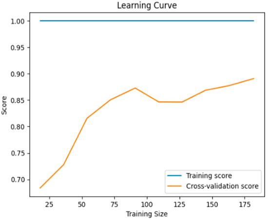
Figure 3.
The learning curve of the model after training.
3.1.2. Paired t-Test Analysis
We performed a t-test analysis to evaluate if there is a statistically significant difference between the evaluation metrics and the test set. Below, in Table 6 and Figure 4, the results are presented.
Table 6.
Paired t-test evaluation metrics for the audio classifier.
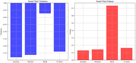
Figure 4.
Graphical representation of the paired t-test statistics and values.
Paired t-test results: This represents the comparison of the performances of the model before and after the cross-validation. A p-value above 0.05 indicates that there is no significant statistical difference between them. A high p-value indicates that cross-validation did not change the performance of the model significantly.
T-test for Accuracy: The p-value is greater than 0.05, meaning that there is no statistically significant difference between the accuracy of the cross-validation and the accuracy of the test set
T-test for Precision: The p-value is greater than 0.05, meaning that there is no statistically significant difference between the precision of the cross-validation and the precision of the test set
T-test for Recall: The p-value is high, meaning that the difference in recall between the cross-validation and the test set is because of random chance, without any statistically significant difference. That also indicates that the test set’s recall is not different from the cross-validation’s recall.
T-test for the F1-Score: There is no statistically significant difference between the F1-scores acquired from the cross-validation and the test set, indicating that the F1-score is similar across both datasets.
3.2. Model’s Performance After Testing in an External Dataset
After training our model with a small portion of the data (10% or 285 entries), we saved the trained model and then we introduced a portion of the data unseen by the model during the training. Even though we used a testing–training split during the training to evaluate the model’s performance, a model trained with a smaller portion of data and then tested with a large portion of unseen data is crucial to ensure overfitting is avoided and a good model evaluation in generalization. The model showcased exemplary performance in the new dataset (90% of the data or 2573 entries), further ensuring its robustness, generalizability, and ability for real-world scenario applications, as shown in Table 7.
Table 7.
Model’s evaluation metrics after the testing.
Performance of the Trained Model in the Test Set (External Dataset)
The trained model’s overall performance exhibits a very high score, and the trained model predicts correctly the data instances, with a good ability to distinguish positive and negative classes. The curve shape pinpoints that the model achieves a high true-positive rate and, at the same time, maintains a low number of false positives. A minor score drop is observed, and it is acceptable considering the fact that the model was trained on a very small portion of data with the class imbalance and yet maintains its reliability [48,49] Figure 5.
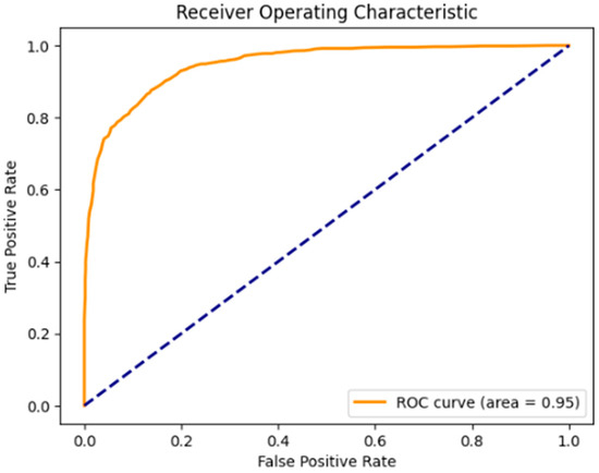
Figure 5.
ROC-AUC score of the model after testing.
Balanced Accuracy in the External Dataset: The score of 0.88 suggests that the model is generalizing well to the unseen data, but at the same time, some noise or feature variability may have been introduced, therefore, causing the drop in the score.
ROC-AUC Score: The score of 0.95 shows that although the balanced accuracy dropped, the model’s overall ability for predictions remains reliable.
Precision: The score of 0.87 means that the model predicts correct positive classes 87% of the time.
Recall: The score of 0.87 means that the model successfully identifies 87% of the actual positive cases.
F1-Score: The score of 0.87 indicates that the model has both high sensitivity and specificity.
Accuracy: The score of 0.87 shows that the model performs well in the overall classification. Consistency with other metrics is shown, where the F1-, precision, and recall scores are aligned, reinforcing the reliability of the model.
Positive Predictive Value (PPV): The score of 0.88 shows that most of the positive predictions are correct.
Negative Predictive Value (NPV): The score of 0.85 shows that the model is predicting negative instances correctly 85% of the time.
Confusion Matrix Figure 6
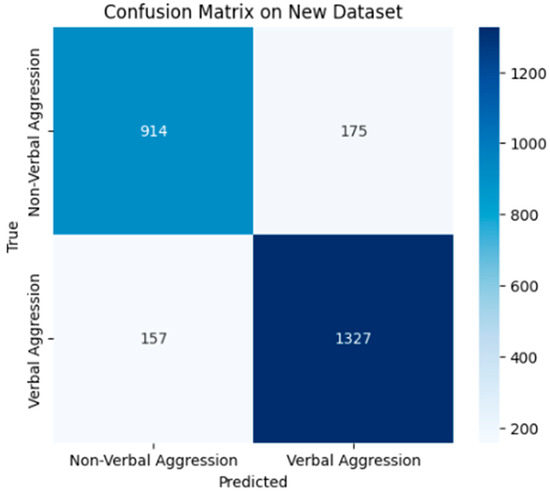
Figure 6.
Confusion matrix of the model after testing.
True Positives (TPs): 1327—Instances of the positive class correctly identified by the model.
True Negatives (TNs): 914—Instances of the negative class correctly identified by the model.
False Positives (FPs): 175—Instances of the negative class incorrectly identified by the model.
False Negatives (FNs): 157—Instances of the positive class incorrectly identified by the model.
Accuracy for Aggression Detections: 90%—From all the true labels as aggressive, the model identified 90% of them as actually aggressive.
Accuracy for Argument Detections: 84%—From all the true labels as non-aggressive, the model identified 84% of them as actually non-aggressive.
The performance of the model tested in an external dataset shows promising results, showcasing a good prediction balance between the two classes falling between the 0.8 and 0.9 accuracy values. These values are based on the results derived as a direct output from our code after the testing finalization, saved in a ‘detection_results.csv’ file. The final results are shown below in Figure 7.

Figure 7.
Probability range/count of correct argument and non-argument predictions per the 0.1 accuracy range, with 1.0 being the perfect accuracy score.
3.3. Meta-Classifier Performance Evaluation After Late Fusion
After applying the late fusion rule to the visual_detection_results.csv and audio_detection_results.csv files, we loaded the dataset merged_detection_results.csv file, consisting of the merged results, and performed an identical pipeline with those of the two previous models to develop a meta-classifier. The meta-classifier reads the data, imputes missing values (if any), standardizes the features, and, using 5k-fold cross-validation, trains the random forest classifier using a testing–training split of 80–20 to make predictions for the combined detection results. The final results are shown in Table 8, Table 9 and Table 10.
Table 8.
Model evaluation results after testing.
Table 9.
Model evaluation metrics’ confusion matrix.
Table 10.
Model evaluation’s classification report.
ROC-AUC Score: 95.52%—An indication that the models’ discrimination abilities between the classes are excellent, as shown in Figure 8.
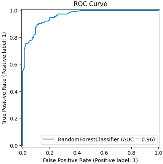
Figure 8.
ROC-AUC score of the trained meta-classifier with the late fusion technique.
Accuracy: 88.0%—A high value, indicating the ability of the model to predict correctly.
Precision: 87.60%—The prediction of the positive class (aggressive) by the model indicates that it is correct 87% of the time.
Recall: 92.17%—An indication that the model is identifying correct true positives and that the missed predictions are few.
F1-Score: 89.83%—The harmonic mean of the model, between the precision and recall, is high, showcasing a good balance.
Balanced Accuracy: 87.26%—An indication that the model performs well across both classes and not only in the dominant class.
Inference Time—Overall, the inference time is 0.0030 s, which means that the model ensures quick predictions in real-world scenario applications.
Positive Predictive Value (PPV): 87.60%—The prediction of the positive class (aggressive) by the model indicates that it is correct 87% of the time.
Negative Predictive Value (NPV): 88.61%—This indicates a high prediction accuracy in the non-aggressive class.
Cross-Validated Balanced Accuracy: 86.82%—This score is similar to the balanced accuracy of the test set, proving the reliability of the model.
Cross-validated ROC-AUC score: 95.52%—This depicts the good generalization ability and robustness of the model.
Confusion Matrix Figure 9
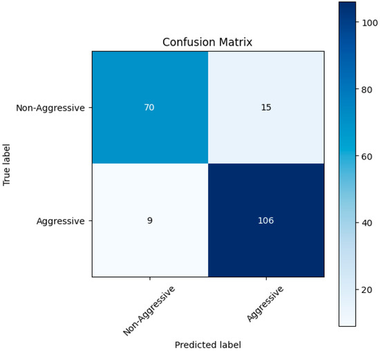
Figure 9.
Confusion matrix results of the trained meta-classifier with the late fusion technique.
True Positives (TPs): 106—Instances of the positive class correctly identified by the model.
True Negatives (TNs): 70—Instances of the negative class correctly identified by the model.
False Positives (FPs): 15—Instances of the negative class incorrectly identified by the model.
False Negatives (FNs): 9—Instances of the positive class incorrectly identified by the model.
Accuracy for Aggression Detections: 92%—From all the true labels as aggressive, the model identified 92% of them as actually aggressive.
Accuracy for Argument Detections: 82%—From all the true labels as non-aggressive, the model identified 82% of them as actually non-aggressive.
Learning Curve: The training score showcases that the model performs extremely well with the training data, but the performance slightly drops from around 460 to 550 samples and then increases steadily while making a plateau. This behavior is expected because the data have never been seen by the model and were not balanced, with the non-aggression class having fewer entries than the aggression class; therefore, this drop is insignificant. This is also the reason the training score remains stable at 1.0 (which is desirable), but the cross-validation score is trying to reach it Figure 10.

Figure 10.
Learning curve results of the trained meta-classifier with the late fusion technique.
Paired t-test Analysis
We performed a t-test analysis on the meta-classifier to evaluate if there is a statistically significant difference between the evaluation metrics and the test set. In all our metrics, the p-value is greater than 0.05, eliminating the indication of statistically significant differences in the performance of the model between the cross-validation and the test set. Below, in Table 11 and Figure 11, the results are presented.
Table 11.
Paired t-test evaluation metrics for the meta-classifier.
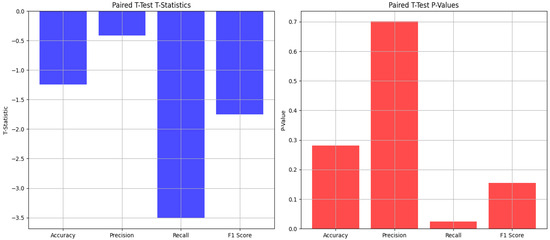
Figure 11.
Graphical representation of the paired t-test statistics and values.
T-test for Accuracy: The t-stat indicates small differences in accuracy between the cross-validation and the test set. The p-value is higher than the typical 0.05 threshold, indicating no statistically significant difference between the accuracy in the cross-validation and the test set.
T-test for Precision: The t-stat indicates small differences in precision between the cross-validation and the test set. The p-value is higher than the typical 0.05 threshold, indicating no statistically significant difference between the precision in the cross-validation and the test set. This also indicates that the precisions in the test set and the cross-validation are consistent.
T-test for Recall: The t-stat indicates a more noticeable difference in recall between the cross-validation and test set without reaching considerably high values. The p-value indicates some statistically significant difference between recall in the cross-validation and the test set. This means that the observed difference in recall did not occur by random chance; therefore, there is a meaningful distinction between recall values in the two sets.
T-test for the F1-Score: The t-stat indicates very small differences in the F1-score between the cross-validation and the test set. The p-value suggests that the F1-score in the test set is consistent with the F1-score observed during the cross-validation.
In Figure 12, we can see the performance metrics of the meta-classifier after the final testing. In Figure 13, we can see the meta-classifier’s count of predictions per probability range. The results show an improvement in certainty, as the probabilities increase from 0.6 to 1.0, which is a good indication. The lower non-aggression prediction count is acceptable because the aggression class had more entries than the non-aggression class.
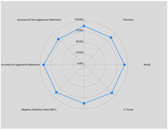
Figure 12.
Meta-classifier’s final model evaluation metrics.
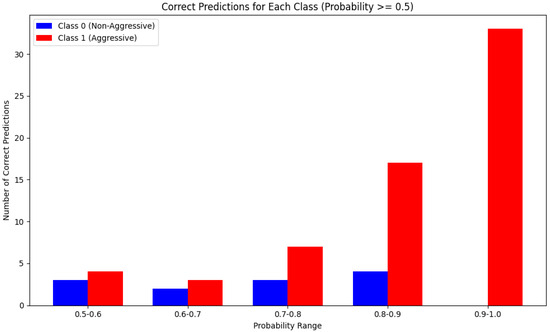
Figure 13.
Probability range/count of correct argument and non-argument predictions per the 0.1 accuracy range, with 1.0 being the perfect accuracy score.
In summary, in the final meta-classifier evaluation, we observe that the combination of audio and visual data further enhanced the model, providing a more robust application of the multimodal approach for predicting aggressive behaviors in real-world applications. Although the recall for the non-aggression class has some room for improvement, this is an acceptable outcome, considering the class imbalance (606 instances in the aggression class vs. 390 non-aggression-class instances) [50,51]. However, the balanced accuracy indicates that the model is robust and that it handles class imbalances well [52].
The effect of the class imbalance on our model is visible in Figure 9 and Figure 12, and in Figure 13, with the model favoring the majority class (aggression), recall in the non-aggression class is slightly lower (0.84) while being higher in the aggression class (0.98). A balanced accuracy of 87.26% supports the model’s bias. Class-balancing mitigation strategies and bias elimination could be applied to the model, such as oversampling techniques, like the synthetic minority oversampling technique (SMOTE) or utilizing the random forest’s attribute class_weight = ‘balanced’, which would increase the minority class’s weight. Nonetheless, on the basis of an unbiased comparison among the audio model, the visual model, and the meta-classifier, no class-balancing mitigation strategy was used because in the previous model, none of these class imbalance mitigation techniques were applied. To mitigate this, a cross-validation of 5 × 5 folds was used in the visual model from the prior work, in the audio classifier, and in the meta-classifier, providing methodological class imbalance mitigation and eliminating random predictions. In spite of this meta-classifier bias, it provides a head-to-head comparison between the previous model and the enhanced prediction model.
3.4. Comparison of the Initial Visual Model and the Late Fusion Model
Following the testing phase of the meta-classifier with the late-fusion-merging technique, the evaluation metrics of the meta-classifier were compared, combining predictions from both visual and audio features with the performance of the visual model. These results are presented in Figure 14.
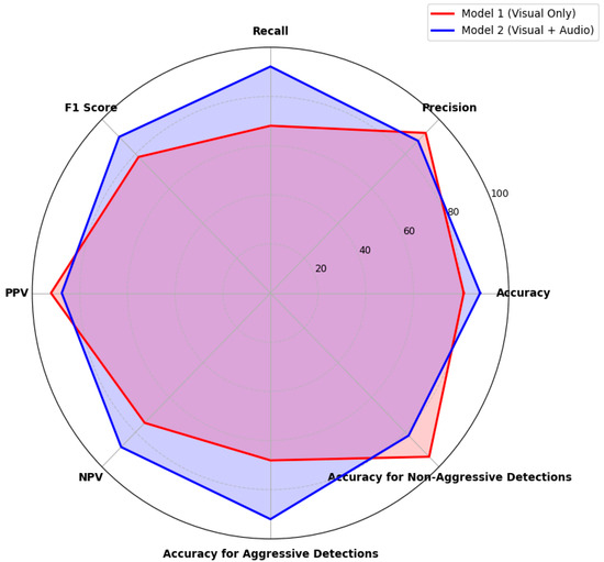
Figure 14.
Performance comparison between the initial model, which uses visual cues only to predict aggressive behaviors, and the late fusion meta-classifier model, which utilizes both visual and audio features for predictions.
The multimodal meta-classifier indicates stability, as shown in Figure 14, with performance metrics distributed across the spider diagram. Significant improvements in the recall, accuracy, F1-score, accuracy for aggression detections, and NPV are shown. However, minor reductions in the precision and PPV are observed, as well as a drop in the accuracy for non-aggression detections. These performance drops are because of the class imbalance in the late fusion merging. The drops in the performances of these three metrics are in the context of a meta-classifier model with balanced metrics.
As shown in Figure 15, the initial visual model has shorter inference times (3.40 ms) than the meta-classifier’s inference time (95.50 ms). The meta-classifier model is 28 times slower. The meta-classifier has to process both audio and visual features, increasing the computational complexity. A tradeoff can be observed in the metrics, where the meta-classifier outperforms the visual-only model in all the scores. This improved performance highlights that the new model significantly enhances the quality of the classification by incorporating audio features. Although speed is the key in real-world applications, the tradeoff for quality improvement is admissible.

Figure 15.
Performance comparison of inference times between the initial model, which uses visual cues only, and the late fusion meta-classifier model, which utilizes both visual and audio features for the prediction of aggressive behaviors.
The statistical testing of results is shown in Figure 16. The t- and p-values were used to measure the difference in significance. A t-value indicates the size of the difference relative to the variability between the two models. For a significant difference, there must be a very large absolute value. A p-value below 0.05 is the threshold for a significant statistical difference.
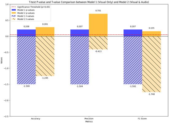
Figure 16.
Comparison of t-test statistical significances between the initial model, which uses visual cues only to predict aggressive behaviors, and the late fusion meta-classifier model, which utilizes both visual and audio features.
- Accuracy (Model 1: t = −1.5000, p = 0.2080; Model 2: t = −1.2454, p = 0.2809)
- Both models have high p-values, significantly higher than the threshold value (0.05), indicating that there is no significant difference between the two models. Model 1 has a negative t-value and lower p-value, which point toward higher significance than the Model 2 comparison’s threshold.
- Precision (Model 1: t = −1.5042, p = 0.2070; Model 2: t = −0.4129, p = 0.7008)
- Model 1 has a higher negative t-value and lower p-value, which demonstrates a higher significance than the Model 2 comparison’s threshold. Model 2 exhibits the minimal precision difference, with a high p-value of 0.7008.
- F1-Score (Model 1: t = −1.5021, p = 0.2075; Model 2: t = −1.7476, p = 0.1555)
- Model 2 exhibits a higher negative t-value and a low p-value, which translates to no statistical significance, indicating that Model 2 is slightly better in the F1-score than Model 1.
According to these findings, Model 1 has better precision, and Model 2 has a balanced performance with a higher F1-score. No significant statistical difference was observed between the two models.
4. Discussion
Patients with dementia are more likely to injure themselves and others during episodes of aggression. The factors associated with these behaviors have been the subject of numerous studies. An important objective is to make caregivers less stressed by identifying the risks associated with these behaviors. Further investigation of the interaction between different cases of behaviors has been conducted by examining vocally and physically aggressive and non-aggressive behaviors in order to better understand the elements involved in agitation and aggressive behaviors in individuals with dementia. The results indicated that verbal aggressiveness was the most disruptive [53,54].
In this study, a machine-learning model that is capable of detecting and classifying aggressive and non-aggressive human behaviors according to audio data was developed, trained, and validated. This model is a multimodal analysis combining previous work, which will further enhance the capabilities of a proof-of-concept implementation and detect aggressive behavior in patients with dementia with higher accuracy and increased reliability. As in the previous work, limitations in acquiring clinical datasets from real dementia patients present an obstacle because of ethical concerns as well as patient consent. Collaborations with psychiatric institutions are mandatory to gather such data and demonstrate the applicability of the model under real-life conditions. A proof of concept provided the basis for the development of the model to simulate real-world scenarios, increasing the reliability of the model, preparing it for clinical applications, and allowing future model evaluations with clinical data [55,56].
The introduction of audio-based classifier predictions, combined with predictions from the visual classifier using a meta-classifier, enhanced model predictions by a factor of 3%. The visual prediction model in the final testing presented an ROC-AUC score of 0.94 [18], with a positive predictive value of 0.92 and a negative predictive value of 0.74. The final results, after evaluating the combined predictions using a meta-classifier, showcased an ROC-AUC score of 0.96, with a positive predictive value of 0.87 and a negative predictive value of 0.88. These results suggest an ROC-AUC score improvement of 2.13%. The positive predictive value slightly decreased by −5.75%. A performance drop is anticipated because of the increased complexity of the information used, producing a realistic evaluation. A significant improvement in the negative predictive value by 18.92% indicates that the model can more accurately predict negative occurrences. The late fusion of the two models led to a more precise and reliable application in predicting aggressive and non-aggressive episodes of behavior. Although these metrics show improvement, there are still some things to consider.
4.1. Key Points for Comparison
The comparison of the metrics was developed using the same evaluation metrics across all three models. Even though the two models (audio and visual) were trained in two different datasets, they were evaluated in a similar test during the meta-classifier phase.
During the merging of the predictions from multiple models, we are leveraging the strengths from both models, and this can sometimes lead to improved performance. Because the meta-classifier, indeed, improves the model’s performance but not significantly, it is safe to assume that this biased occurrence was avoided.
When combining predictions, there is the need to address if this improvement is statistically significant. Even though a small increase in the ROC-AUC score is not a substantial improvement, it is worth considering that there was a large improvement in the negative predictive cases. The quality of our evaluation and improvement is also further proved by the results of the paired t-tests, which show a statistically significant improvement and not a random chance.
In conclusion, all the above proves that this implementation would make an impact in real-world scenarios. This will be further confirmed with an early fusion method and real-world clinical data acquired from the psychiatric department.
4.2. The Model’s Advantages
The improvements in the evaluation metrics with the late fusion multimodal and meta-classifier implementation depict that the model is effective in classifying cases. The analysis is now being executed using two different types of data (visual images and audio clips), providing robustness for the model’s ability to differentiate instances at different decision thresholds, as shown in Figure 13. Moreover, the model showcases high precision in both positive and negative predictions, with the false positives and false negatives remaining at low values. The combination of the random forest’s ensemble nature alongside the techniques used in handling overfitting and data discrepancies contributes to the model’s overall performance and reliability. The fused model shows a balanced performance throughout all the metrics (Figure 13 and Figure 14), with improved prediction performance. The statistical analysis showed no significant difference, with the exception of the F1-score showing a minor increase. As a result, predicting and preventing episodes of aggression can be more accurate, and intervention strategies from caregivers to dementia patients could improve the efficiency [57,58,59].
4.3. The Model’s Disadvantages
Regarding the model’s weaknesses, its stability could be the focus of improvement. As indicated by the new fused-data learning-curve graph in Figure 11, the cross-validation scores approximate the training set scores, in a fluctuating course with the first training samples reaching the model’s stability. This could indicate that the model needs more training data samples for improved learning. Further, a t-stat score of −1.81 indicates a significant difference in recall between the cross-validation and test set scores. As mentioned above, the model shows longer inference times compared to those of the initial model because of its complexity in having to process both visual and audio features for making predictions, thus increasing computational time. Further, no mitigation strategies were used to handle the class imbalance, providing a fair comparison with the initial model. This signifies a minor bias toward the positive class. Moreover, in Figure 14, Figure 15 and Figure 16, the statistical analysis indicates that the combined late fusion model shows slight declines in some metrics, maintaining a balanced improvement in performance. This does not interfere with the model’s functionality and is something that could be improved with a larger and more balanced training sample. Moreover, the introduction of larger real clinical data containing audio and visual information from patients with dementia could resolve these issues [60,61].
4.4. The Choice of the Methodology
The pipeline was selected based on previous work and remained constant in this study in order to follow the model’s hierarchy and, therefore, provide consistent results. Therefore, the ensemble classification nature of the random forest classifier was reused because its ability to adapt to different operating conditions and its consistency in performance at various decision thresholds make it an ideal approach for our application [42]. Other classification model choices could be implemented in this study, but they would make the point of the enhancement obsolete because a different classifier would provide neither reliability nor unification to a later holistic implementation of the model in real-world scenarios. Our aim is to prove that an audio implementation indeed enhances our application and, therefore, leaves room in the future for early fusion research and the unification of the two models into one powerful model that will be tested on real clinical data containing both audio and visual feedback.
4.5. Challenges in Real-World Clinical Settings
There is a need to address the use of simulated and/or controlled datasets and how these impact real-world clinical settings. As discussed previously, the datasets used in both the visual and audio models were from free online open-source datasets, like the Kaggle and 3D Poses in the Wild Dataset. They were used to develop our models and provide a proof-of-concept model that could be tested in the future in real-world clinical scenarios. Clinical visual and audio data can further improve the models in future work. Clinical datasets could identify challenges that can impede the nature of the results, such as environmental and background noises that exist in clinical environments. Further, individual variability could impede predictions because each patient exhibits varying behaviors. Another important factor in considering real clinical data is quality control. Real-world data suffer from missing values and mislabeling, impacting their quality and ease of use. To this end, mitigation techniques have already been implemented in all the models currently studied.
4.6. Strategies for Real-World Application
Adaptation strategies to the challenges discussed can be implemented, such as robust data augmentation, simulating noise in clinical data during the training, and domain adaptation techniques to transfer learning from a controlled dataset to a clinical dataset with the use of fine tuning. These strategies have been implemented in the models. Finally, collaboration with healthcare institutions is necessary in order to acquire clinical data from psychiatric institutions, as well as active learning within an active feedback loop, where human experts can monitor and decide on the validity of the results.
4.7. Ethical Considerations
Considering the wider moral ramifications of machine-learning algorithm applications for predicting aggressive behaviors in vulnerable populations, we must address related ethical issues, such as privacy and misclassification risk.
Privacy: Predictive models frequently use sensitive data, including audio biometric data, pictures, video records, and behavioral logs. We must abide by stringent privacy regulations and ethical standards to prevent abuse or unlawful usage. All the datasets and participants must remain anonymous, and the participants must provide their agreement after being fully informed about how their data will be used. Strict data privacy is another crucial responsibility of researchers, particularly for vulnerable populations [60,61];
Risk of False Positives and False Negatives: False positives could have a number of negative effects, including unwarranted medical intervention or stigmatization, as a result of incorrect predictions of aggressive conduct. These could lead to incorrect actions or have a detrimental impact on the health of individuals who are already at risk. Clinical decision making is supported by the use of predictive models. Such dangers can be reduced by combining machine learning with the knowledge of skilled employees [62,63];
Bias and Fairness: Biases in training data can be applied by algorithms, leading to incorrect findings. When working with communities or vulnerable populations, this is particularly troublesome. When creating such models, mitigation techniques are incorporated. Regular actions must be taken to guarantee the fairness, transparency, and minimization of bias in such systems [60,61]. Considering misclassification and bias mitigation in the datasets, both datasets were not balanced from their sources. To mitigate bias and fairness, cross-validation techniques with 5 × 5 folds were used to eliminate randomness and reduce misclassification risks;
Ethical Deployment and Oversight: Prior to putting such models into practice in community contexts, like psychiatric hospitals, schools, or prisons, it is imperative to involve interdisciplinary and mental health teams of experts. To prevent unnecessary risks to individuals who are already in danger, the morality of these models must be ensured [60,61];
Accountability and Human Agency: The purpose of machine-learning models is to assist human judgment. Case-by-case use should be left to experts, who can understand the model’s behavior and predictions in a broader context. When working with vulnerable groups, formal accountability structures should be implemented to ensure such functionality;
Patient Consent and Privacy: The dataset was acquired from Kaggle’s “Audio-based Violence Detection Dataset” a free open-source dataset, with audio files ready for academic use. No consent form was needed because of the dataset’s nature. No ethics board or institutional review board (IRB) approval was needed or engaged in this study. The data (both visual and audio) were already anonymized from their sources without posing any potential risk or harm through the intended use. The dataset was publicly available and pre-existing, with no direct interaction with patients, and did not contain any personally identifiable information (PII). To prevent unethical bias in data cross-validation, 5 × 5 folds were utilized in all our models current and prior, to eliminate random predictions.
5. Conclusions
In this study, the main goal was to create a secondary classifier model based on audio data, which will enhance the prediction capabilities of our initial visual model in predicting aggressive outbursts in dementia patients. Using the same methodology as in the initial visual model, an audio model was developed, trained, and tested using data noise and artifact filtering, imputation of missing data, and standardization. Following the initial results, merging the prediction results of the two models followed, using the late fusion technique and feeding the final dataset into a meta-classifier. The meta-classifier was trained and tested on the combined data types (audio and visual) and showcased improved prediction results. As more complex and differentiated data were introduced to the model, a more realistic real-world application scenarios could provide insights about the future of this multimodal analysis.
It should be taken into consideration that controlled conditions were used in the previous work. Real-world environmental data often contain noise and variability. In this research, data of such a nature were introduced, with audio clips containing information about various daily life instances. Audio noise and artifacts were filtered with real-life variability. Even though the nature of the data was not controlled in this model development, the results nonetheless improved. This could be a strong indication that our proof of concept could be tested under real-world conditions and be tested using real clinical data.
For future work, the model could be implemented with an early fusion rule, in order to cross-validate the results and the model’s capabilities. Also, the acquisition of a real-world clinical dataset will further indicate utilization in providing a novel approach for advanced care in dementia patient facilities, encompassing a greater variety of noise and behaviors in its functionality. Although the model provides promising results, stability issues may occur because of the small size of the training data sample. Another important step toward future improvement would be an early fusion model. In this model, prediction merging from the audio and visual models would merge features in a unified concatenated dataset. This integration could provide a better representation and lead to an improved understanding of the classification performance. This proof of concept will provide useful insights about the future implementation of the model, its generalizability skills, and its resilience, opening a new door for machine learning in psychiatric applications and healthcare systems while also improving patients’ qualities of life.
Author Contributions
Conceptualization, I.G.; Methodology, I.G., R.F.S. and N.K.; Software, I.G.; Validation, I.G.; Formal analysis, I.G.; Investigation, I.G. and A.V.; Resources, I.G.; Data curation, I.G.; Writing—original draft, I.G.; Writing—review & editing, I.G., R.F.S., N.K. and M.S.; Visualization, I.G.; Supervision, I.G. and I.V. All authors have read and agreed to the published version of the manuscript.
Funding
This research received no external funding.
Institutional Review Board Statement
Not applicable.
Informed Consent Statement
Not applicable.
Data Availability Statement
The original data presented in the study are openly available at https://www.kaggle.com/datasets/fangfangz/audio-based-violence-detection-dataset (accessed on 15 January 2025).
Conflicts of Interest
The authors declare no conflict of interest.
References
- Devshi, R.; Shaw, S.; Elliott-King, J.; Hogervorst, E.; Hiremath, A.; Velayudhan, L.; Kumar, S.; Baillon, S.; Bandelow, S. Prevalence of Behavioural and Psychological Symptoms of Dementia in Individuals with Learning Disabilities. Diagnostics 2015, 5, 564–576. [Google Scholar] [CrossRef]
- Schablon, A.; Wendeler, D.; Kozak, A.; Nienhaus, A.; Steinke, S. Prevalence and Consequences of Aggression and Violence towards Nursing and Care Staff in Germany—A Survey. Int. J. Environ. Res. Public Health 2018, 15, 1274. [Google Scholar] [CrossRef]
- Priyadarshinee, P.; Clarke, C.J.; Melechovsky, J.; Lin, C.M.Y.; Balamurali, B.T.; Chen, J.M. Alzheimer’s Dementia Speech (Audio vs. Text): Multi-Modal Machine Learning at High vs. Low Resolution. Appl. Sci. 2023, 13, 4244. [Google Scholar] [CrossRef]
- Arevalo-Rodriguez, I.; Smailagic, N.; Roqué-Figuls, M.; Ciapponi, A.; Sanchez-Perez, E.; Giannakou, A.; Pedraza, O.L.; Cosp, X.B.; Cullum, S. Mini-Mental State Examination (MMSE) for the early detection of dementia in people with mild cognitive impairment (MCI). Cochrane Database Syst. Rev. 2021, 7, CD010783. [Google Scholar] [CrossRef]
- Chun, C.T.; Seward, K.; Patterson, A.; Melton, A.; MacDonald-Wicks, L. Evaluation of Available Cognitive Tools Used to Measure Mild Cognitive Decline: A Scoping Review. Nutrients 2021, 13, 3974. [Google Scholar] [CrossRef]
- Nowroozpoor, A.; Dussetschleger, J.; Perry, W.; Sano, M.; Aloysi, A.; Belleville, M.; Brackett, A.; Hirshon, J.M.; Hung, W.; Moccia, J.M.; et al. Detecting Cognitive Impairment and Dementia in the Emergency Department: A Scoping Review. J. Am. Med. Dir. Assoc. 2022, 23, 1314.e31–1314.e88. [Google Scholar] [CrossRef]
- Martin, S.A.; Townend, F.J.; Barkhof, F.; Cole, J.H. Interpretable machine learning for dementia: A systematic review. Alzheimer’s Dement. 2023, 19, 2135–2149. [Google Scholar] [CrossRef]
- Javeed, A.; Dallora, A.L.; Berglund, J.S.; Ali, A.; Ali, L.; Anderberg, P. Machine Learning for Dementia Prediction: A Systematic Review and Future Research Directions. J. Med. Syst. 2023, 47, 17. [Google Scholar] [CrossRef]
- Merkin, A.; Krishnamurthi, R.; Medvedev, O.N. Machine learning, artificial intelligence, and the prediction of dementia. Curr. Opin. Psychiatry 2022, 35, 123–129. [Google Scholar] [CrossRef]
- Chang, C.H.; Lin, C.H.; Lane, H.Y. Machine Learning and Novel Biomarkers for the Diagnosis of Alzheimer’s Disease. Int. J. Mol. Sci. 2021, 22, 2761. [Google Scholar] [CrossRef]
- Irfan, M.; Shahrestani, S.; Elkhodr, M. Enhancing Early Dementia Detection: A Machine Learning Approach Leveraging Cognitive and Neuroimaging Features for Optimal Predictive Performance. Appl. Sci. 2023, 13, 10470. [Google Scholar] [CrossRef]
- Stefanou, K.; Tzimourta, K.D.; Bellos, C.; Stergios, G.; Markoglou, K.; Gionanidis, E.; Tsipouras, M.G.; Giannakeas, N.; Tzallas, A.T.; Miltiadous, A. A Novel CNN-Based Framework for Alzheimer’s Disease Detection Using EEG Spectrogram Representations. J. Pers. Med. 2025, 15, 27. [Google Scholar] [CrossRef]
- Wei, Z.; Iyer, M.R.; Zhao, B.; Deng, J.; Mitchell, C.S. Artificial Intelligence-Assisted Comparative Analysis of the Overlapping Molecular Pathophysiology of Alzheimer’s Disease, Amyotrophic Lateral Sclerosis, and Frontotemporal Dementia. Int. J. Mol. Sci. 2024, 25, 13450. [Google Scholar] [CrossRef]
- Boyle, L.D.; Giriteka, L.; Marty, B.; Sandgathe, L.; Haugarvoll, K.; Steihaug, O.M.; Husebo, B.S.; Patrascu, M. Activity and Behavioral Recognition Using Sensing Technology in Persons with Parkinson’s Disease or Dementia: An Umbrella Review of the Literature. Sensors 2025, 25, 668. [Google Scholar] [CrossRef] [PubMed]
- Iaboni, A.; Spasojevic, S.; Newman, K.; Martin, L.S.; Wang, A.; Ye, B.; Mihailidis, A.; Khan, S.S. Wearable multimodal sensors for the detection of behavioral and psychological symptoms of dementia using personalized machine learning models. Alzheimer’s Dement. Diagn. Assess. Dis. Monit. 2022, 14, e12305. [Google Scholar] [CrossRef]
- Sharma, N.; Klein Brinke, J.; Braakman Jansen, L.M.A.; Havinga, P.J.M.; Le, D.V. Wi-Gitation: Replica Wi-Fi CSI Dataset for Physical Agitation Activity Recognition. Data 2024, 9, 9. [Google Scholar] [CrossRef]
- Inoue, Y.; Moshnyaga, V.G. A Real-Time Detection of Patient’s Aggressive Behaviors on a Smart Sensor. In Proceedings of the 2024 IEEE 67th International Midwest Symposium on Circuits and Systems (MWSCAS), IEEE, Springfield, MA, USA, 11–14 August 2024; pp. 911–914. [Google Scholar] [CrossRef]
- Galanakis, I.; Soldatos, R.F.; Karanikolas, N.; Voulodimos, A.; Voyiatzis, I.; Samarakou, M. A MediaPipe Holistic Behavior Classification Model as a Potential Model for Predicting Aggressive Behavior in Individuals with Dementia. Appl. Sci. 2024, 14, 10266. [Google Scholar] [CrossRef]
- Chu, H.C.; Zhang, Y.L.; Chiang, H.C. A CNN Sound Classification Mechanism Using Data Augmentation. Sensors 2023, 23, 6972. [Google Scholar] [CrossRef]
- Keen, S.C.; Odom, K.J.; Webster, M.S.; Kohn, G.M.; Wright, T.F.; Araya-Salas, M. A machine learning approach for classifying and quantifying acoustic diversity. Methods Ecol. Evol. 2021, 12, 1213–1225. [Google Scholar] [CrossRef]
- Mou, A.; Milanova, M. Performance Analysis of Deep Learning Model-Compression Techniques for Audio Classification on Edge Devices. Science 2024, 6, 21. [Google Scholar] [CrossRef]
- Abayomi-Alli, O.O.; Damaševičius, R.; Qazi, A.; Adedoyin-Olowe, M.; Misra, S. Data Augmentation and Deep Learning Methods in Sound Classification: A Systematic Review. Electronics 2022, 11, 3795. [Google Scholar] [CrossRef]
- Zaman, K.; Sah, M.; Direkoglu, C.; Unoki, M. A Survey of Audio Classification Using Deep Learning. IEEE Access 2023, 11, 106620–106649. [Google Scholar] [CrossRef]
- Tsalera, E.; Papadakis, A.; Samarakou, M. Comparison of Pre-Trained CNNs for Audio Classification Using Transfer Learning. J. Sens. Actuator Netw. 2021, 10, 72. [Google Scholar] [CrossRef]
- Sakri, S.; Basheer, S. Fusion Model for Classification Performance Optimization in a Highly Imbalance Breast Cancer Dataset. Electronics 2023, 12, 1168. [Google Scholar] [CrossRef]
- Nykoniuk, M.; Basystiuk, O.; Shakhovska, N.; Melnykova, N. Multimodal Data Fusion for Depression Detection Approach. Computation 2025, 13, 9. [Google Scholar] [CrossRef]
- Younis, E.M.G.; Zaki, S.M.; Kanjo, E.; Houssein, E.H. Evaluating Ensemble Learning Methods for Multi-Modal Emotion Recognition Using Sensor Data Fusion. Sensors 2022, 22, 5611. [Google Scholar] [CrossRef]
- Saidi, S.; Idbraim, S.; Karmoude, Y.; Masse, A.; Arbelo, M. Deep-Learning for Change Detection Using Multi-Modal Fusion of Remote Sensing Images: A Review. Remote Sens. 2024, 16, 3852. [Google Scholar] [CrossRef]
- Resende Faria, D.; Weinberg, A.I.; Ayrosa, P.P. Multimodal Affective Communication Analysis: Fusing Speech Emotion and Text Sentiment Using Machine Learning. Appl. Sci. 2024, 14, 6631. [Google Scholar] [CrossRef]
- Choi, H.S. Emotion Recognition Using a Siamese Model and a Late Fusion-Based Multimodal Method in the WESAD Dataset with Hardware Accelerators. Electronics 2025, 14, 723. [Google Scholar] [CrossRef]
- Xu, Z.; Yu, G. A Time Series Forecasting Approach Based on Meta-Learning for Petroleum Production under Few-Shot Samples. Energies 2024, 17, 1947. [Google Scholar] [CrossRef]
- Abdul, Z.K.; Al-Talabani, A.K. Mel Frequency Cepstral Coefficient and its Applications: A Review. IEEE Access 2022, 10, 122136–122158. [Google Scholar] [CrossRef]
- Liu, W.; Li, A.; Wang, X.; Yuan, M.; Chen, Y.; Zheng, C.; Li, X. A Neural Beamspace-Domain Filter for Real-Time Multi-Channel Speech Enhancement. Symmetry 2022, 14, 1081. [Google Scholar] [CrossRef]
- Vogel, R.; Schlosser, T.; Manthey, R.; Ritter, M.; Vodel, M.; Eibl, M.; Schneider, K.A. A Meta Algorithm for Interpretable Ensemble Learning: The League of Experts. Mach. Learn. Knowl. Extr. 2024, 6, 800–826. [Google Scholar] [CrossRef]
- FangFangZ. (n.d.). Audio-Based Violence Detection Dataset [Dataset]. Kaggle. Available online: https://www.kaggle.com/datasets/fangfangz/audio-based-violence-detection-dataset (accessed on 15 January 2025).
- Huang, C.-S. An Adaptive Cutoff Frequency Design for Butterworth Low-Pass Filter Pursuing Robust Parameter Identification for Battery Energy Storage Systems. Batteries 2023, 9, 198. [Google Scholar] [CrossRef]
- Zhang, S.; Gao, Y.; Cai, J.; Yang, H.; Zhao, Q.; Pan, F. A Novel Bird Sound Recognition Method Based on Multifeature Fusion and a Transformer Encoder. Sensors 2023, 23, 8099. [Google Scholar] [CrossRef] [PubMed]
- Cao, Y.; Zhao, P.; Xu, B.; Liang, J. An Improved Random Forest Approach on GAN-Based Dataset Augmentation for Fog Observation. Appl. Sci. 2024, 14, 9657. [Google Scholar] [CrossRef]
- Nezami, N.; Haghighat, P.; Gándara, D.; Anahideh, H. Assessing Disparities in Predictive Modeling Outcomes for College Student Success: The Impact of Imputation Techniques on Model Performance and Fairness. Educ. Sci. 2024, 14, 136. [Google Scholar] [CrossRef]
- Radzi, S.F.M.; Karim, M.K.A.; Saripan, M.I.; Rahman, M.A.A.; Isa, I.N.C.; Ibahim, M.J. Hyperparameter Tuning and Pipeline Optimization via Grid Search Method and Tree-Based AutoML in Breast Cancer Prediction. J. Pers. Med. 2021, 11, 978. [Google Scholar] [CrossRef]
- Pereira, L.M.; Salazar, A.; Vergara, L. A Comparative Analysis of Early and Late Fusion for the Multimodal Two-Class Problem. IEEE Access 2023, 11, 84283–84300. [Google Scholar] [CrossRef]
- Lueangwitchajaroen, P.; Watcharapinchai, S.; Tepsan, W.; Sooksatra, S. Multi-Level Feature Fusion in CNN-Based Human Action Recognition: A Case Study on EfficientNet-B7. J. Imaging 2024, 10, 320. [Google Scholar] [CrossRef]
- Huang, X.; Ma, T.; Jia, L.; Zhang, Y.; Rong, H.; Alnabhan, N. An effective multimodal representation and fusion method for multimodal intent recognition. Neurocomputing 2023, 548, 126373. [Google Scholar] [CrossRef]
- Zhang, T.; Luo, B.; Sharda, A.; Wang, G. Dynamic Label Assignment for Object Detection by Combining Predicted IoUs and Anchor IoUs. J. Imaging 2022, 8, 193. [Google Scholar] [CrossRef]
- Liu, K.; Liu, J.; Liu, S. Enhanced Semi-Supervised Medical Image Classification Based on Dynamic Sample Reweighting and Pseudo-Label Guided Contrastive Learning (DSRPGC). Mathematics 2024, 12, 3572. [Google Scholar] [CrossRef]
- Deng, Y.; Zhang, C.; Yang, N.; Chen, H. FocalMatch: Mitigating Class Imbalance of Pseudo Labels in Semi-Supervised Learning. Appl. Sci. 2022, 12, 10623. [Google Scholar] [CrossRef]
- Pan, Q.; Meng, Z. Hybrid Uncertainty Calibration for Multimodal Sentiment Analysis. Electronics 2024, 13, 662. [Google Scholar] [CrossRef]
- Zou, R.; Wang, N. Imbalanced Data Parameter Optimization of Convolutional Neural Networks Based on Analysis of Variance. Appl. Sci. 2024, 14, 9071. [Google Scholar] [CrossRef]
- Zheng, M.; Wang, F.; Hu, X.; Miao, Y.; Cao, H.; Tang, M. A Method for Analyzing the Performance Impact of Imbalanced Binary Data on Machine Learning Models. Axioms 2022, 11, 607. [Google Scholar] [CrossRef]
- Williams, C.K.I. The Effect of Class Imbalance on Precision-Recall Curves. Neural Comput. 2021, 33, 853–857. [Google Scholar] [CrossRef]
- Das, S.; Mullick, S.S.; Zelinka, I. On Supervised Class-Imbalanced Learning: An Updated Perspective and Some Key Challenges. IEEE Trans. Artif. Intell. 2022, 3, 973–993. [Google Scholar] [CrossRef]
- Hellín, C.J.; Olmedo, A.A.; Valledor, A.; Gómez, J.; López-Benítez, M.; Tayebi, A. Unraveling the Impact of Class Imbalance on Deep-Learning Models for Medical Image Classification. Appl. Sci. 2024, 14, 3419. [Google Scholar] [CrossRef]
- Scuteri, D.; Contrada, M.; Loria, T.; Tonin, P.; Sandrini, G.; Tamburin, S.; Nicotera, P.; Bagetta, G.; Corasaniti, M.T. Pharmacological Treatment of Pain and Agitation in Severe Dementia and Responsiveness to Change of the Italian Mobilization–Observation–Behavior–Intensity–Dementia (I-MOBID2) Pain Scale: Study Protocol. Brain Sci. 2022, 12, 573. [Google Scholar] [CrossRef]
- Cesana, B.M.; Poptsi, E.; Tsolaki, M.; Bergh, S.; Ciccone, A.; Cognat, E.; Fabbo, A.; Fascendini, S.; Frisoni, G.B.; Frölich, L.; et al. A Confirmatory and an Exploratory Factor Analysis of the Cohen-Mansfield Agitation Inventory (CMAI) in a European Case Series of Patients with Dementia: Results from the RECage Study. Brain Sci. 2023, 13, 1025. [Google Scholar] [CrossRef] [PubMed]
- Li, H.; Rajbahadur, G.K.; Lin, D.; Bezemer, C.P.; Jiang, Z.M. Keeping Deep Learning Models in Check: A History-Based Approach to Mitigate Overfitting. IEEE Access 2024, 12, 70676–70689. [Google Scholar] [CrossRef]
- Freiesleben, T.; Grote, T. Beyond generalization: A theory of robustness in machine learning. Synthese 2023, 202, 109. [Google Scholar] [CrossRef]
- Oh, S.-I.; Kang, H.-B. Object Detection and Classification by Decision-Level Fusion for Intelligent Vehicle Systems. Sensors 2017, 17, 207. [Google Scholar] [CrossRef] [PubMed]
- Khan, I.A.; Birkhofer, H.; Kunz, D.; Lukas, D.; Ploshikhin, V. A Random Forest Classifier for Anomaly Detection in Laser-Powder Bed Fusion Using Optical Monitoring. Materials 2023, 16, 6470. [Google Scholar] [CrossRef]
- Tsai, H.; Yang, T.W.; Ou, K.H.; Su, T.H.; Lin, C.; Chou, C.F. Multimodal Attention Network for Dementia Prediction. IEEE J. Biomed. Health Inform. 2024, 28, 6918–6930. [Google Scholar] [CrossRef]
- Solís-Martín, D.; Galán-Páez, J.; Borrego-Díaz, J. A Model for Learning-Curve Estimation in Efficient Neural Architecture Search and Its Application in Predictive Health Maintenance. Mathematics 2025, 13, 555. [Google Scholar] [CrossRef]
- Schmid, L.; Roidl, M.; Kirchheim, A.; Pauly, M. Comparing Statistical and Machine Learning Methods for Time Series Forecasting in Data-Driven Logistics—A Simulation Study. Entropy 2025, 27, 25. [Google Scholar] [CrossRef]
- Joseph, J. Predicting crime or perpetuating bias? The AI dilemma. AI Soc. 2024, 1–3. [Google Scholar] [CrossRef]
- Farayola, M.M.; Tal, I.; Connolly, R.; Saber, T.; Bendechache, M. Ethics and Trustworthiness of AI for Predicting the Risk of Recidivism: A Systematic Literature Review. Information 2023, 14, 426. [Google Scholar] [CrossRef]
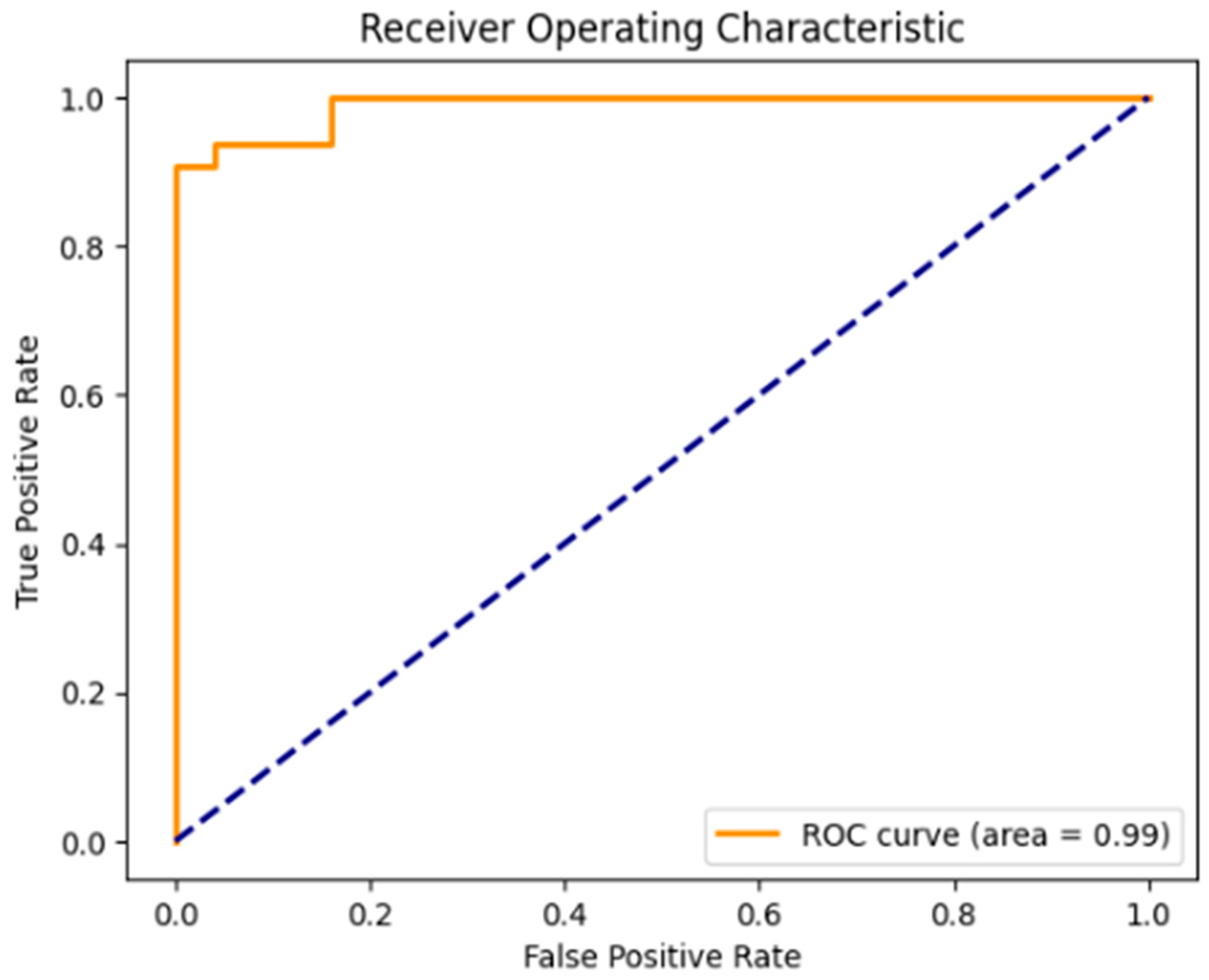
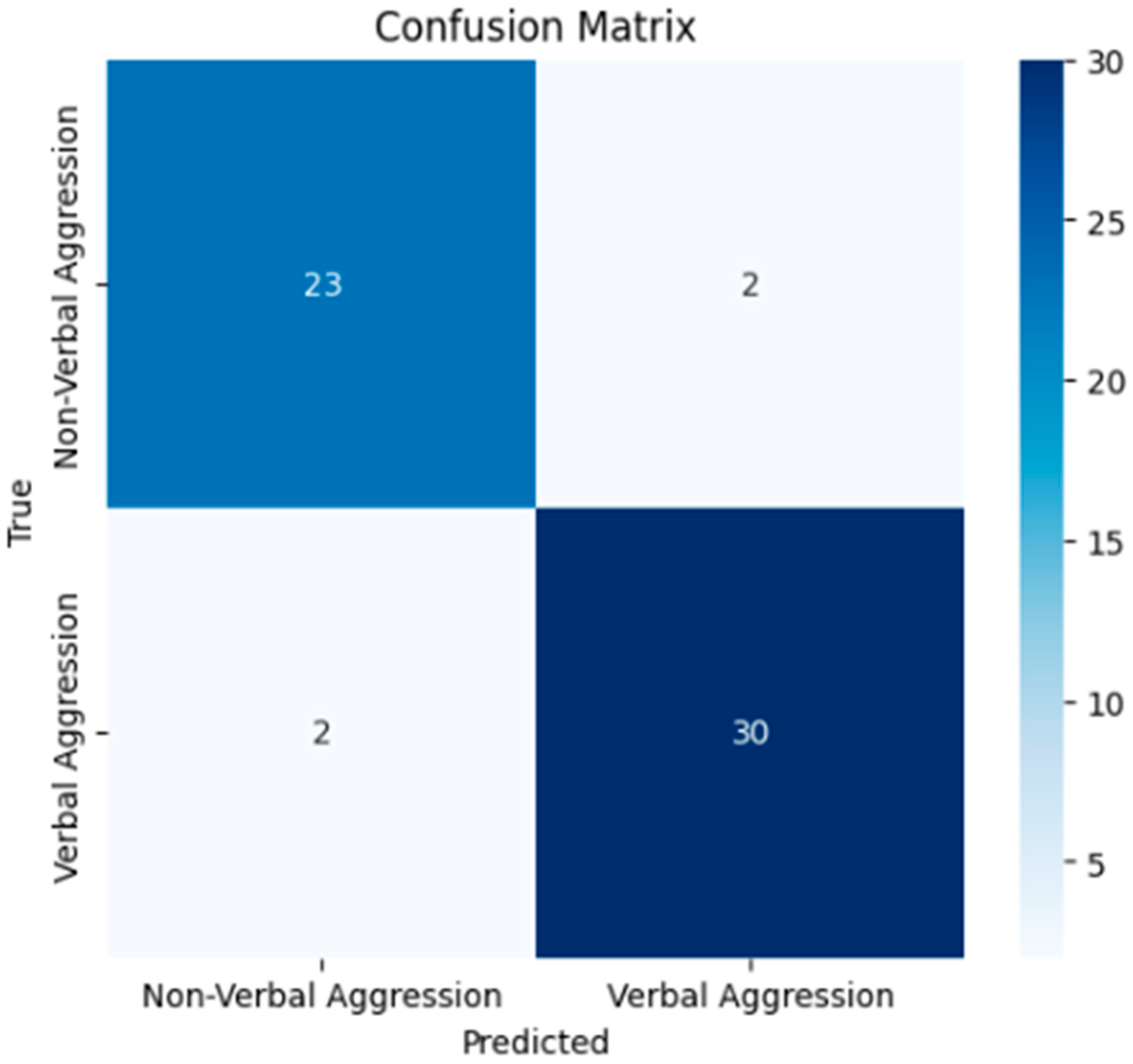
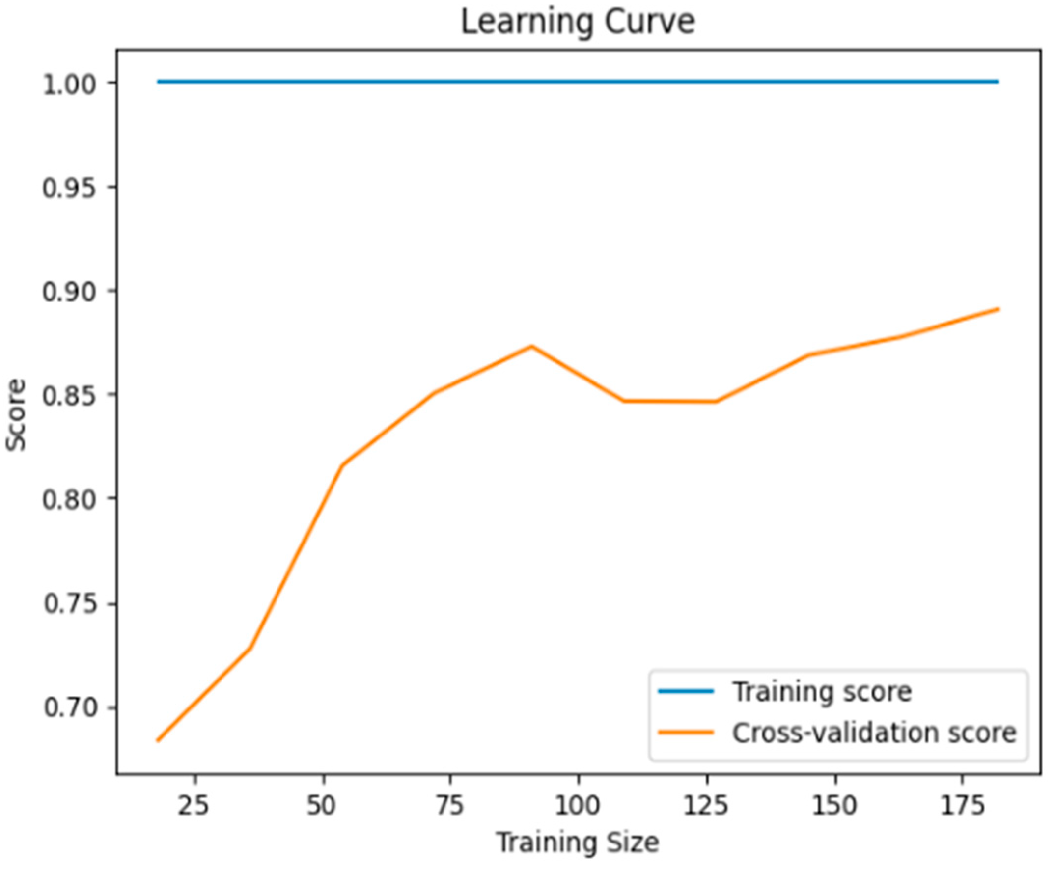
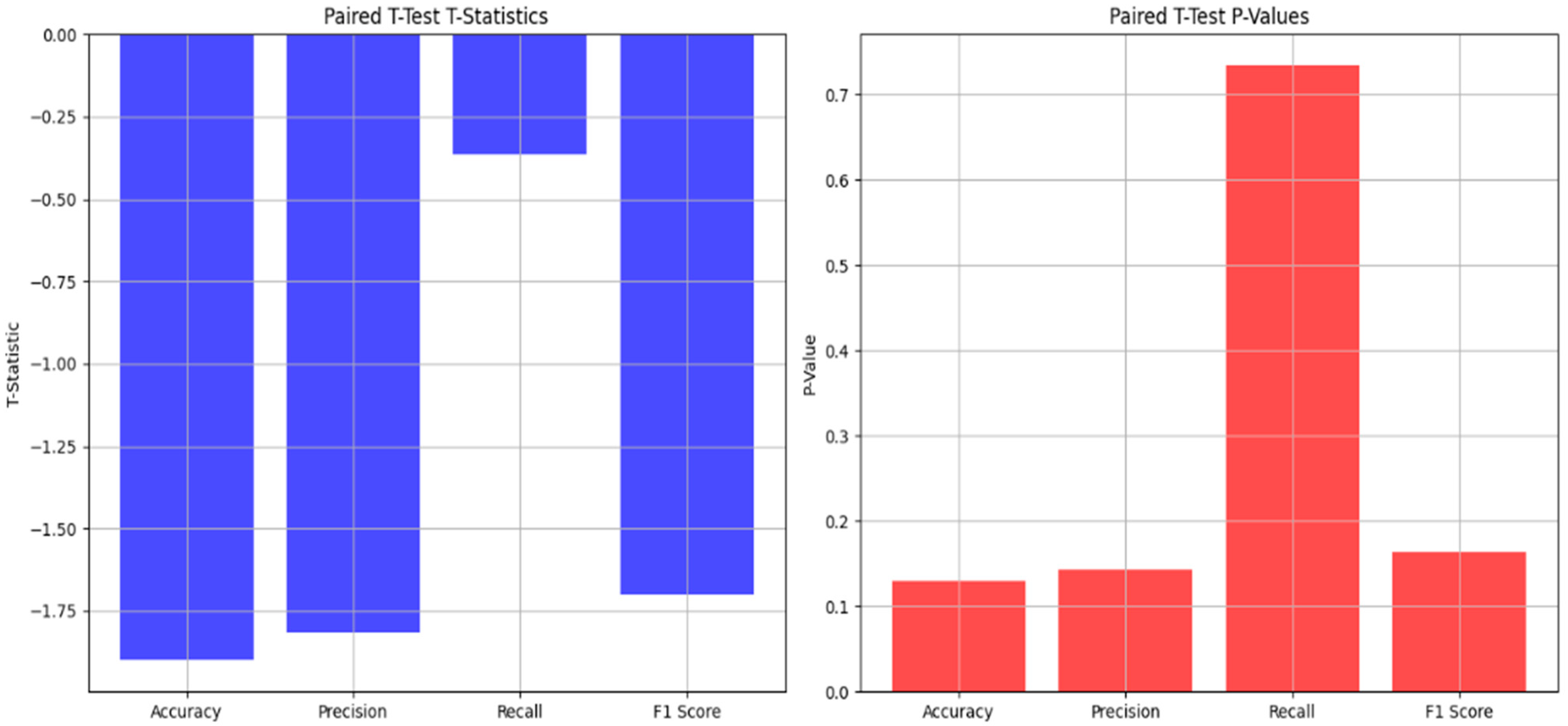


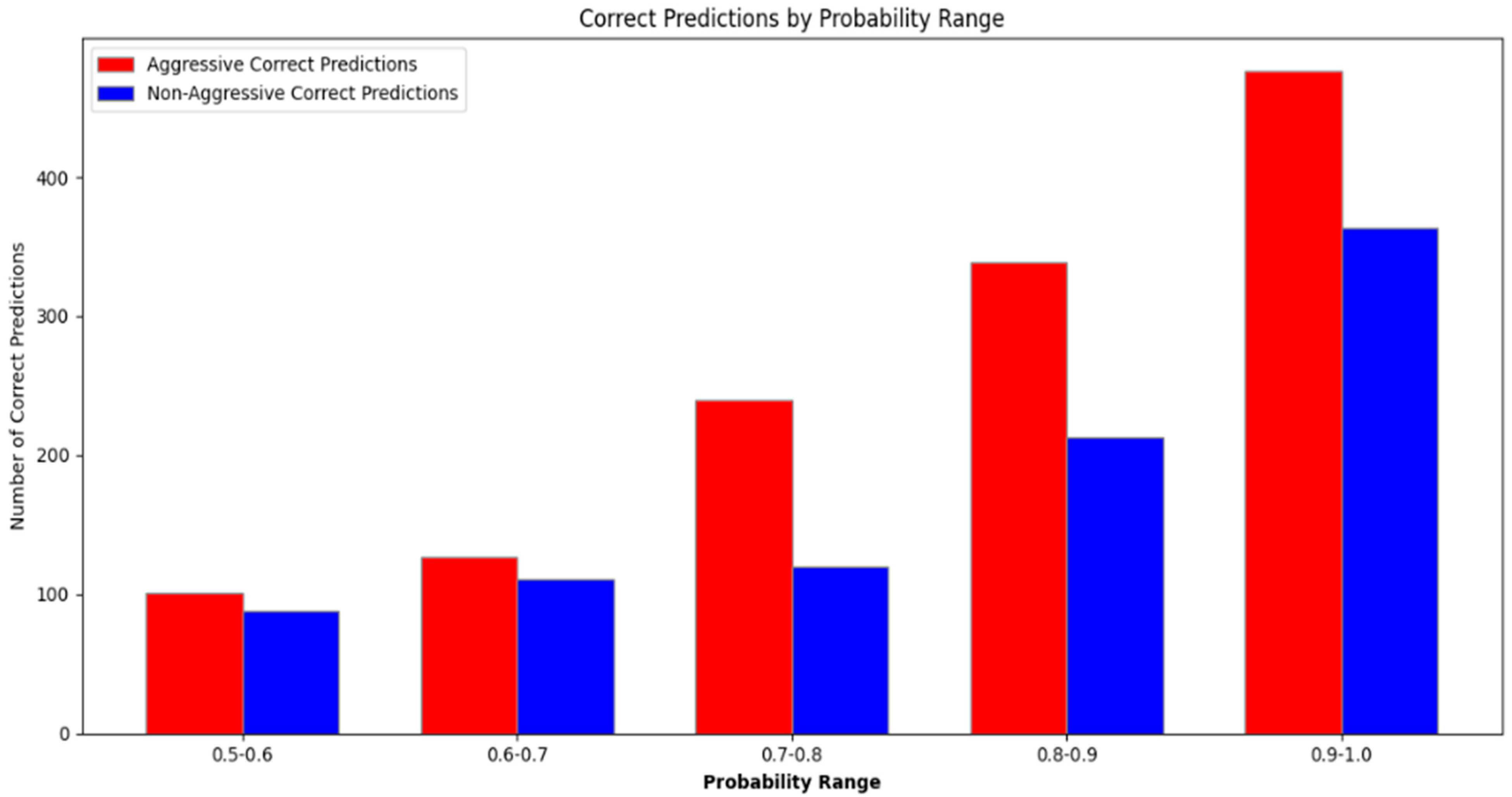
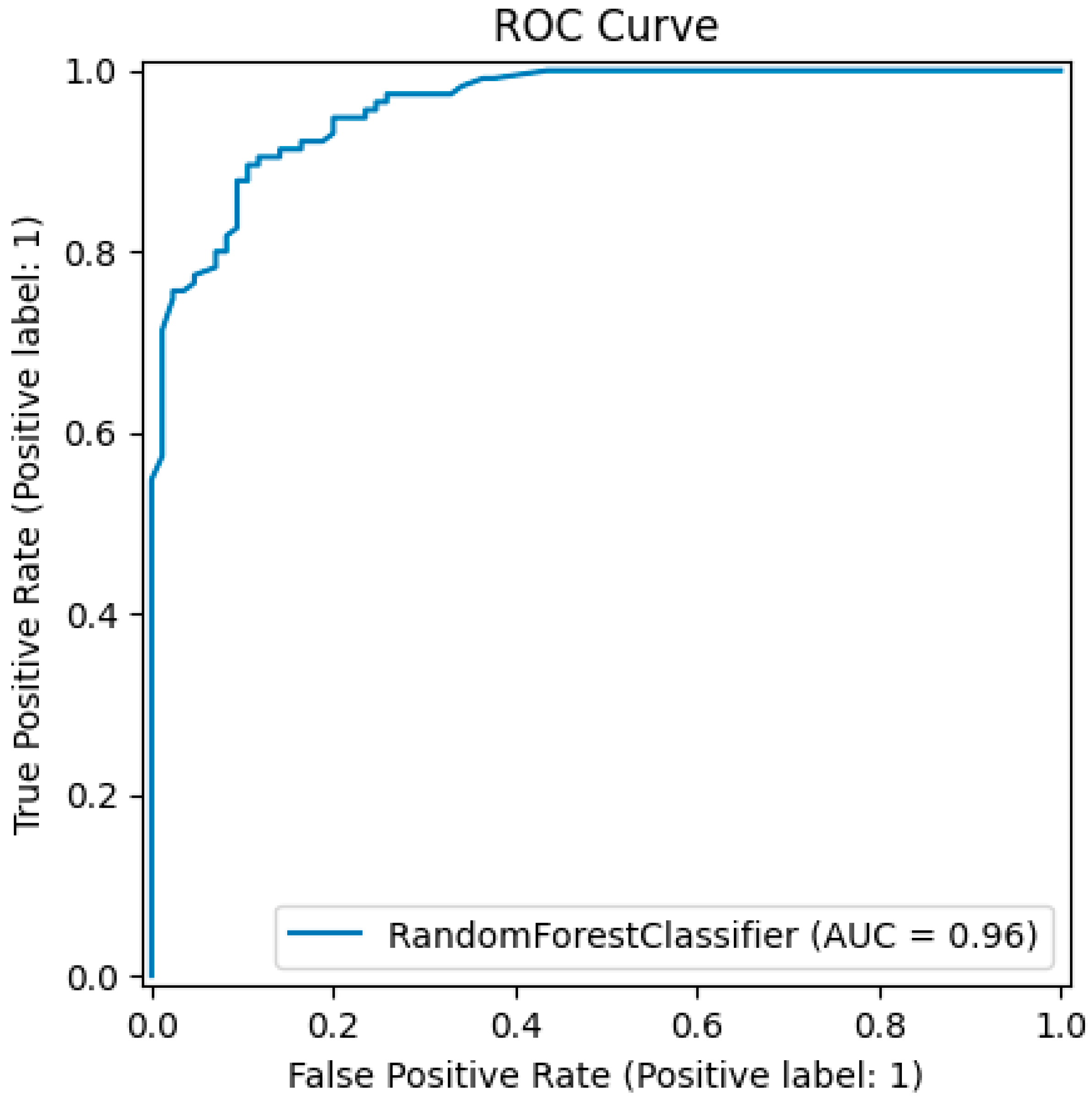

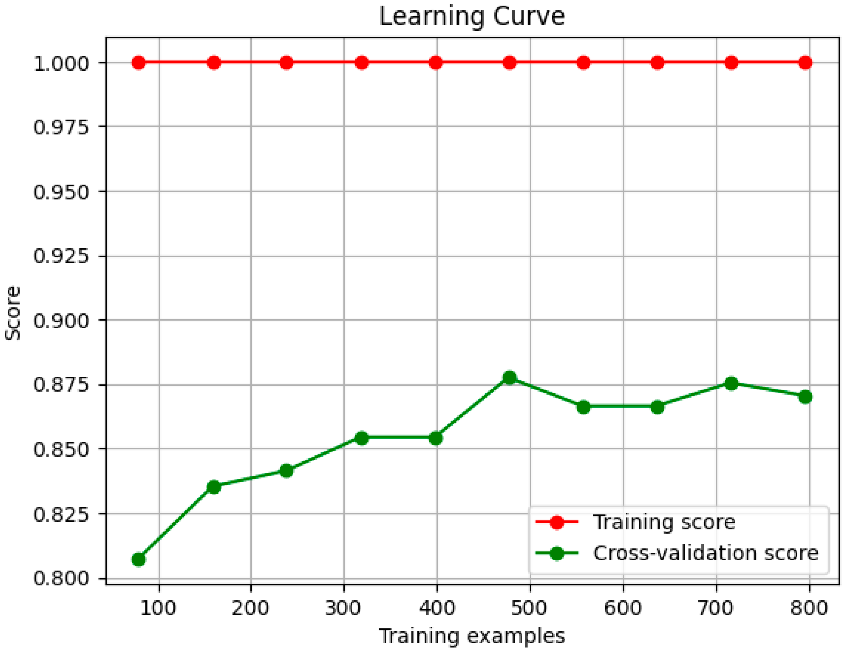

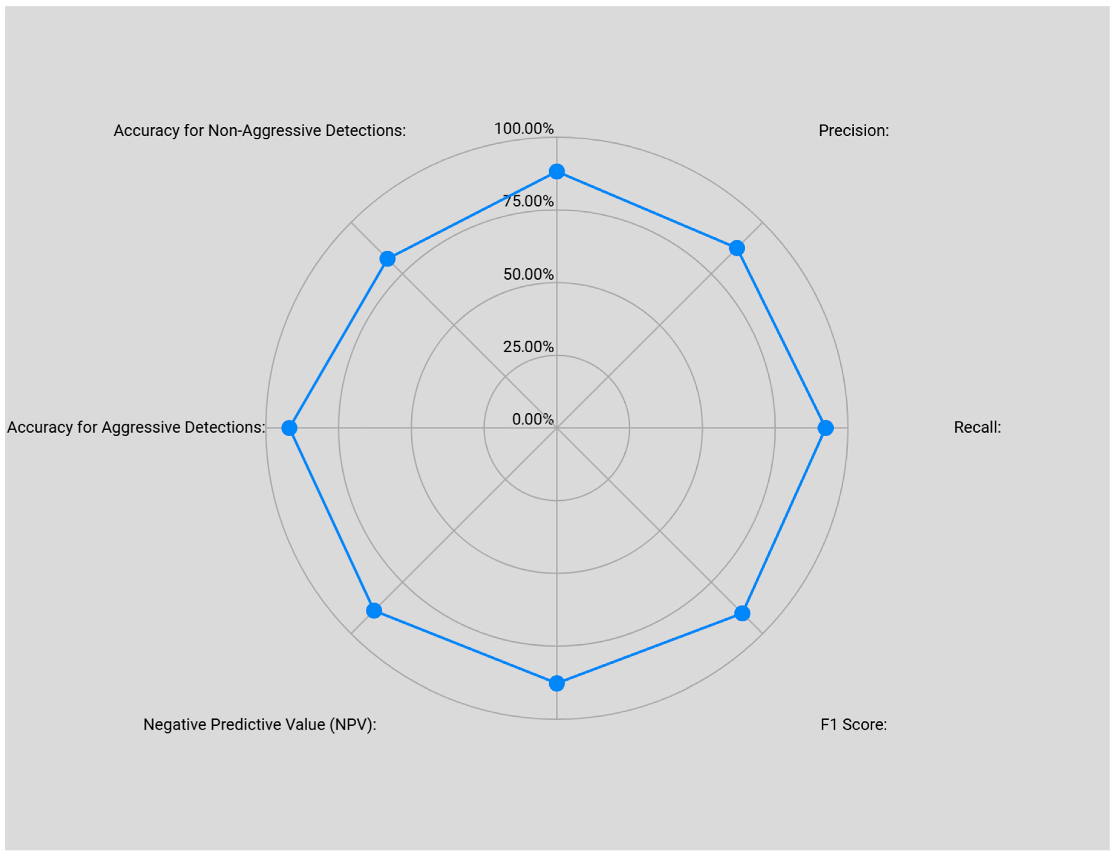

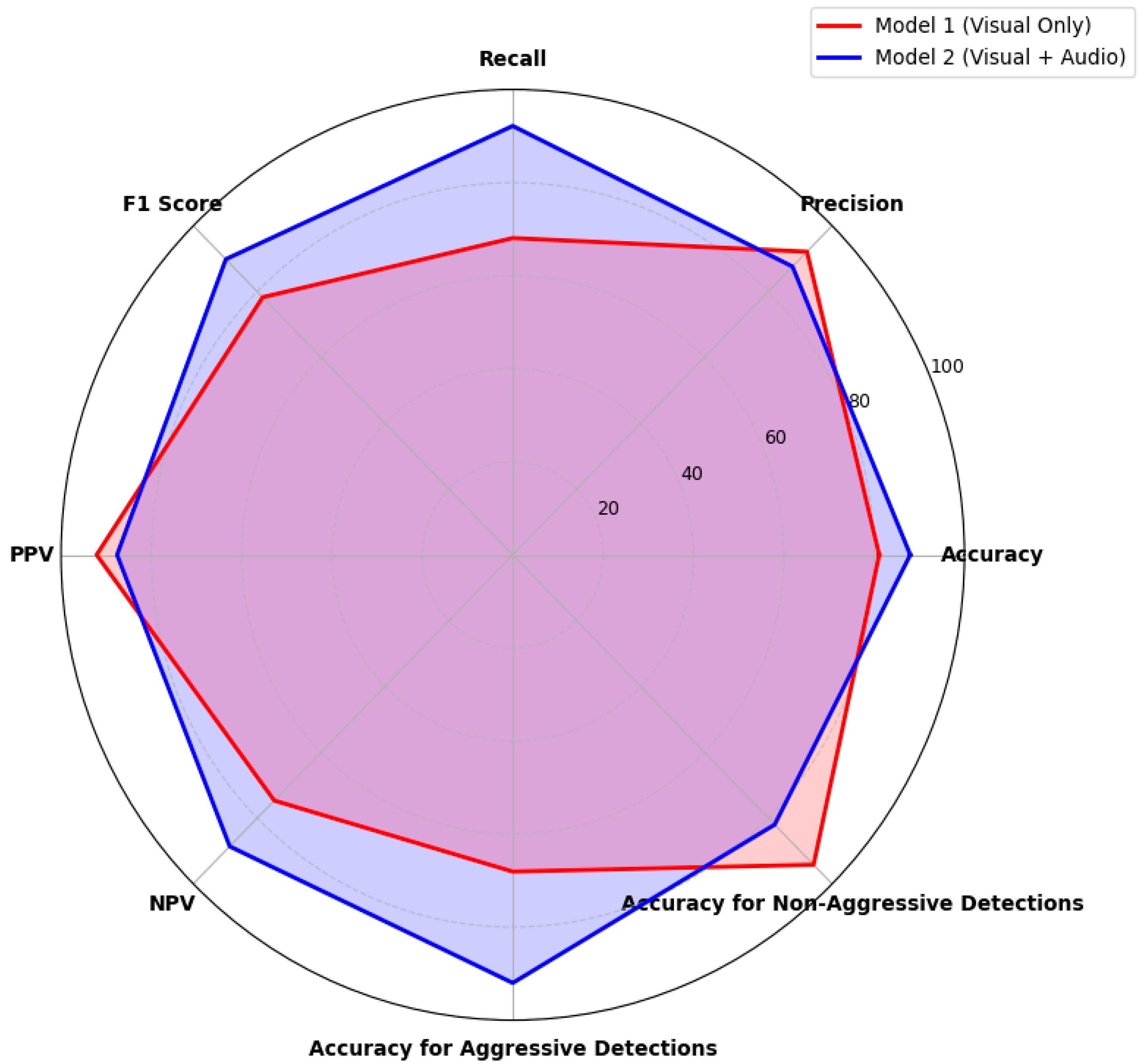
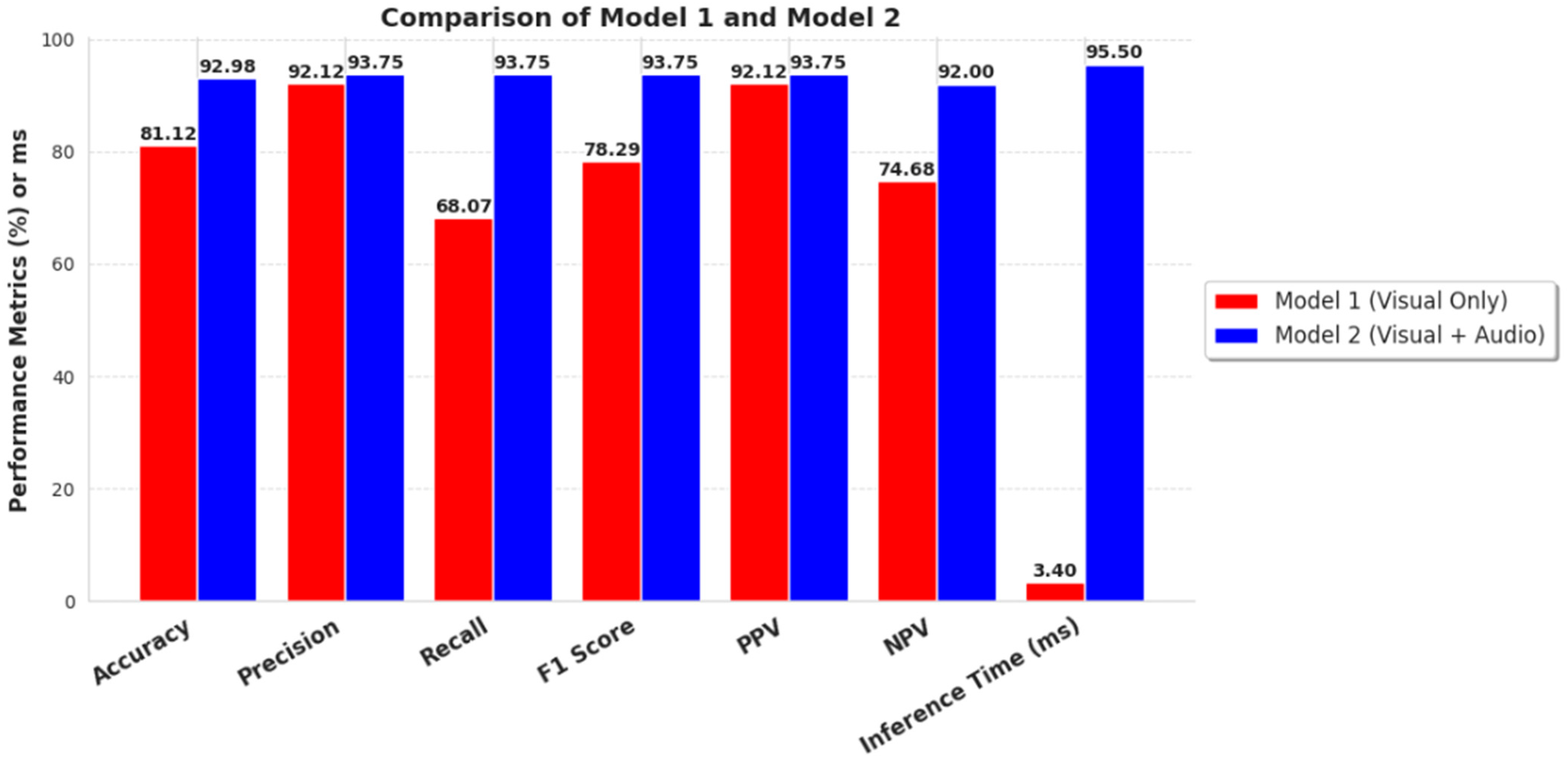
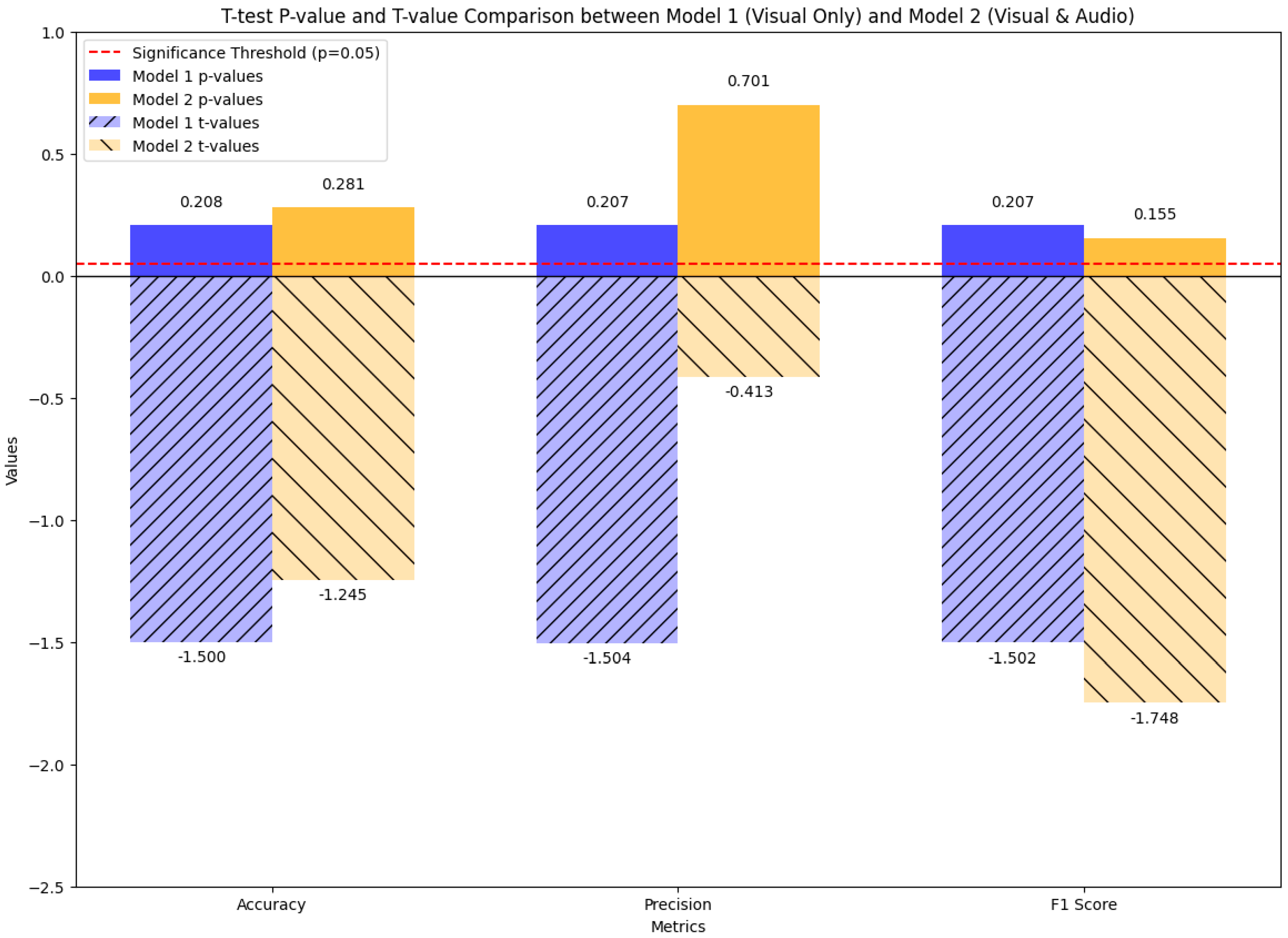
Disclaimer/Publisher’s Note: The statements, opinions and data contained in all publications are solely those of the individual author(s) and contributor(s) and not of MDPI and/or the editor(s). MDPI and/or the editor(s) disclaim responsibility for any injury to people or property resulting from any ideas, methods, instructions or products referred to in the content. |
© 2025 by the authors. Licensee MDPI, Basel, Switzerland. This article is an open access article distributed under the terms and conditions of the Creative Commons Attribution (CC BY) license (https://creativecommons.org/licenses/by/4.0/).