Research on Fleet Size of Demand Response Shuttle Bus Based on Minimum Cost Method

Abstract

Demand-responsive connector services (DRC) are an important means to improve the current mobility connection problem. In this study, we develop a hybrid model for the minimization of total system cost for demand response shuttle buses, which includes operating cost and user cost, with fleet size per hour as the optimization variable of the model. The relevant variables are analyzed and numerically modeled by Matlab, and the relationship between fleet size, vehicle capacity and demand density and waiting time, onboard time, vehicle travel distance, and total system cost is analyzed. The results indicate that introducing financial subsidies markedly lowers the critical demand density necessary to ensure system viability. Moreover, subsidy intensity is positively associated with the service’s operational robustness. Through parametric examination, we observe a strictly monotonic relationship between subsidy magnitude and demand thresholds: as subsidy levels increase, the minimum demand requirements for sustainable operation decrease in a consistent, progressive manner; meanwhile, the optimal fleet size exhibits an approximately linear relationship with travel demand per unit area across varying vehicle capacities. Notably, an increase in vehicle capacity corresponds to a decrease in the growth rate of the required fleet size. This model demonstrates robust adaptability across diverse operational scenarios and serves as an effective tool for evaluating the efficiency of resource allocation in demand-responsive transit (DRT) services. Furthermore, it provides valuable theoretical support for the scheduling and planning of public transportation systems, particularly in low-density urban environments.

1. Introduction

With the acceleration of urbanization and the diversification of travel needs, people are demanding higher quality travel services [1]. Traveling as a service has become a development trend of urban public transport in the future [2]. The traditional fixed-route transit (FRT) mode can meet the travel demand of high-density passenger flow through the reasonable arrangement of the travel plan, but in the area where the travel demand of the residents is small in scale and spatially scattered, the conventional bus mode will produce a series of problems [3]. On the one hand, the line can only stop at fixed stations and the passenger direct access rate is low, resulting in many passenger service blind spots, insufficient passenger flow, and serious vehicle idling. Bus companies, in order to improve economic efficiency, will reduce the frequency of buses and shorten service times. However, this not only fails to solve the problem but also increases passenger waiting times and reduces service levels. Consequently, it becomes difficult to cultivate a stable passenger flow along the route [4]. On the other hand, when residents face public transportation that cannot meet their travel demands, they must choose other modes of travel. This provides conditions and space for the increase in private car ownership and illegal transportation operations [5,6]. Therefore, in reality, there is an urgent need for flexible and economic modes of transport organization to serve the residents of such areas [7,8].

Demand-responsive transport is a flexible mode of operation. After years of development, a different form of layout evolved, mainly containing five kinds: point deviation (PD), new request stops (NRS), flexible route segments (FRS), demand-responsive connector (DRC), and zone route (ZR). Demand-responsive connector (DRC) is a common mode serving low-density areas, which requires vehicles to respond to passengers’ dynamic requests in real time within an area, but requires that they arrive at pre-determined transfer points (at least one) at a fixed time to ensure interchange with other modes in the bus network [9,10,11,12]. An important feature of a DRC service is the ability to achieve door-to-door service, which provides a high degree of flexibility. However, it increases vehicle diversions distances while meeting the needs of dispersed passenger travel [13,14,15]. Therefore, how to reasonably allocate the number of vehicles to meet the demand and ensure the service quality is a key issue that needs to be solved for DRC services [16].

Researchers have proposed various pricing methodologies from diverse perspectives. For instance, Burris et al. [17] analyzed traveler responsiveness to fare adjustments to inform bus pricing strategies. Kaddmira et al. [18] integrated marginal cost pricing into agent-based models to optimize short-distance fares, while Boson [19] explored optimal pricing frameworks under varying service conditions. Qiu et al. used the demand elasticity coefficient to design the bus fare setting model [20]. There are also several studies focusing on bus schedule optimization. Szeto et al. developed a model with the objective of minimizing passenger transfers and total travel time to optimize bus routes and frequency between suburban and urban areas [21]. Zeng et al. proposed an equilibrium bus boarding model to study the optimal pricing and bus departure intervals in the presence of inefficiencies of bus commuting during high peak hours [22]. Wagate et al. proposed a model to optimize bus schedules by considering the stations and routes of urban buses in order to optimize the bus scheduling process [23]. Some scholars have considered the uncertainty of passenger demand and optimized the bus schedules accordingly. Avila et al. constructed a bi-objective mathematical model to solve the multi-period urban bus schedules taking into account the uncertainty of passenger demand [24].

While existing studies address fare optimization through factors like congestion, subsidies, and passenger demographics, they often overlook vehicle-related parameters, such as fleet size and capacity. A holistic approach integrating passenger needs with operational constraints—including long-term economic and environmental impacts—remains underexplored [25].

Recent studies on fleet sizing span diverse vehicle types. For example, Li [26] developed a hybrid bus allocation model incorporating constraints like fleet size, passenger flow, express stop frequency, emissions, and electric bus range. Genetic algorithms were employed to assess how electric vehicle adoption impacts total operational costs. Wang, based on the travel trajectory and travel demand of some new energy vehicles in Shanghai, used genetic algorithms to solve for the fleet size of small-scale self-driving shared vehicles (SAVs), and finally determined that the optimal scenario occurs when one SAV replaces 2.4 private cars on average [27]. Emami considered vehicle scheduling and dispatcher allocation, and constructed a hybrid fleet size optimization model for shared vehicles with profit maximization of the operator as the objective, CO2 emission and road congestion levels as the constraints, and solved the degree of influence of different factors on the fleet size by using Gurobi in Matlab R2022b [28]. Yetkin proposed a planning method for the minimum fleet for reservation carpooling, by constructing a topological relationship graph of journeys between carpooling passengers and solving the minimum path in this topological relationship, and then calculating the minimum fleet size [29]. Zhu proposed a two-layer model based on IC card swipe data for regional schedule optimization and fleet size constraints based on the station influence degree, and the optimized results showed that the number of buses allocated was reduced while meeting the base passenger demand, and a reasonable trip chain and travel plan were further constructed [30]. Golbabaei proposed a minimum fleet size adjustment method for a demand-aware dynamic carpooling system, and the minimum fleet size is calculated by the Hopcroft–Karp algorithm based on the trip diagram [31].

In addition to the above methods of constructing fleet sizes for different vehicle types, some authors have also proposed fleet models based on the minimization of transit operating costs [32]. Konstanze conducted field simulations for an automated demand-responsive transportation system and showed that when the travel cost of the total operating cost is minimized and the maximum passenger waiting time requirement is met, the optimal fleet model for shuttle services can be determined [33]. It was also shown that the most effective ways to reduce system costs to passengers are to increase the level of demand, increase the proportion of independently arriving passengers, and use adequate vehicle sizes and shorter vehicle dwell times. Among them, Quadrifoglio et al. established a model for optimizing and adjusting the operating efficiency parameters of the bus system by analyzing the key parameters of the flexible bus system, and carried out simulation and verification analyses to correct the parameters of the model with regard to the design of the system routes and the scheduling problems established in the previous stage. Mandar considered that people make this trip by car, shuttle bus, bike, or walking modes. Cars and shuttle buses, which share the same road network, constitute about 76% of the total trips. As road congestion is expected to grow in the future, it is prudent to look for other modes that can fulfill the travel demand.

In Japan, DRCs have primarily been explored in the context of public transportation in both urban and rural settings. The Japanese government has shown significant interest in integrating DRC systems to address challenges posed by an aging population and declining ridership on conventional public transport systems. A prominent example of DRC implementation in Japan is the “Himawari Bus” service in the Fukutsu region, which operates using an advanced algorithm that adjusts routes based on real-time user demand. Quadrifoglio et al. (2007) [34] studied the effectiveness of such systems, concluding that they provide a more sustainable alternative to traditional bus services in sparsely populated areas.

In Europe, DRC systems have been adopted and tested in various cities to enhance public transport efficiency, particularly in regions facing similar challenges of underutilized services. Countries like the Netherlands and the UK have pioneered the development and implementation of DRC technologies, focusing on both environmental sustainability and social inclusivity. In the Netherlands, the “OV-bus” system has been extensively studied. Research by Quadrifoglio et al. (2018) [35] analyzed the performance of DRC systems in Dutch cities, emphasizing the role of real-time data and demand forecasting in optimizing service routes. The findings indicate that DRCs, when integrated with smart city technologies, can reduce emissions and improve operational efficiency while maintaining or even increasing passenger satisfaction. The UK has seen similar success with DRCs, particularly in areas like Manchester and London. The TFL Go app, which provides on-demand shuttle services, has been the subject of multiple studies, including Kim et al. (2018) [36] who examined the integration of DRCs with traditional bus and rail networks. Their research highlights that DRCs can offer a cost-effective solution for filling gaps in transit coverage while contributing to the decarbonization goals set by the European Union.

Both Japan and European countries have demonstrated the potential of demand-responsive connectors to revolutionize transportation systems. In Japan, DRCs have been especially useful in rural and aging-population areas, while European research has focused on integrating these systems into urban transport networks to reduce emissions and congestion. The studies reviewed highlight that, while challenges remain in terms of technological integration and user adoption, the future of DRCs holds promise for creating more sustainable and flexible transport solutions. Further research and pilot programs will be essential in refining the efficiency and scalability of these systems

Current research gaps include the absence of fleet optimization models balancing passenger and operator interests for DRC services. To address this, our study introduces a cost-minimization framework that optimizes fleet size by harmonizing user experience (e.g., wait times) with operational efficiency (e.g., vehicle utilization). The model construction relies on the dynamic variables of travel demand decisions, such as operating cycle, slack time, waiting time, in-vehicle time and vehicle travel distance, etc., and then uses numerical simulation to further study the relationship between fleet size, demand density, vehicle capacity and the above dynamic variables, and finally simulates the total system cost of DRC buses under different scenarios of different demands through simulation, so as to analyze and obtain the optimal fleet cost under different demands and different vehicle types. The optimal fleet size under different demands and different vehicle types is analyzed [37].

Conventional models often assume single-vehicle operations within partitioned service zones, disregarding interdependencies between zones. This oversimplification fails to account for cross-zone demand patterns or operational constraints, leading to sub-optimal fleet allocation. Therefore, it is necessary to take into account the distribution of passenger flow, vehicle capacity constraints, operating time limitations and other factors between the various service areas, to establish a model of the number of vehicles allocated to the line, and to coordinate and optimize the allocation of vehicles on the line.

2. Cost Model of DRC

In this Section, the objective function is constructed with the goal of minimizing the total cost of the DRC system, and the optimal fleet size is further obtained based on the relationship between the vehicle occupancy rate [38], the frequency of departure and the type of vehicle, and the model is simulated as a whole as well as analyzed in different scenarios. In order to facilitate the calculation, first we set up the DRC operation.

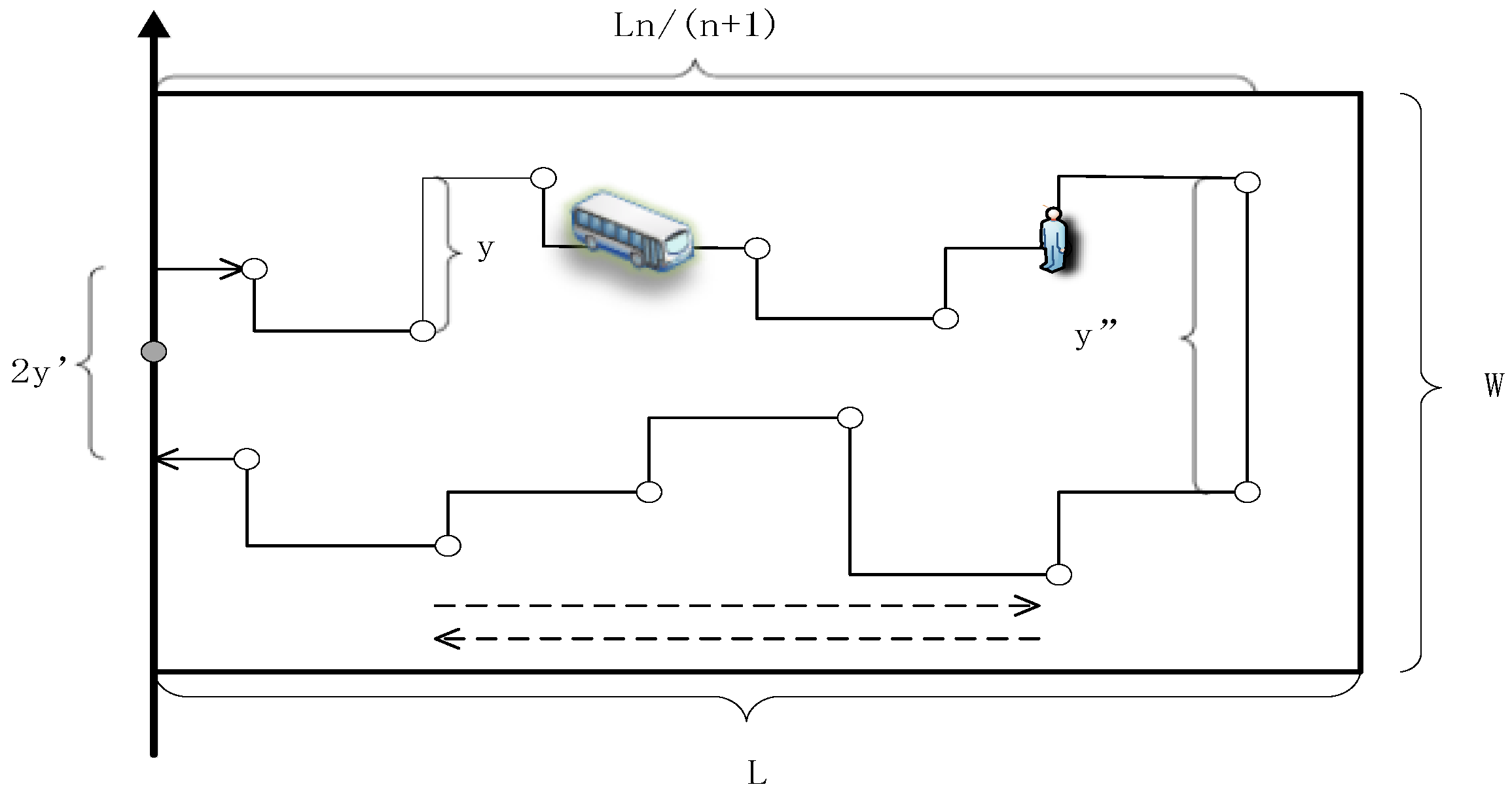
2.1. Assumptions of DRC Vehicle Operation

The service area of DRC buses is usually a rectangular range, and the process of a vehicle starting from and returning to the starting point within the service area is regarded as one operation cycle. Vehicle operation within the area is assumed as follows [39]:

(1)

The service area is a rectangle of length L and width W, with the start and end points located at W/2;

(2)

Within the service area, travel demand conforms to a Poisson distribution;

(3)

The vehicle maintains a uniform speed and its average operating speed is v;

(4)

The boarding and alighting demands of each passenger do not overlap, i.e., the number of stops of the vehicle is equal to the number of traveling demands.

According to the DRC operation characteristics and the above assumptions, the operation of DRC in the service area is simplified as shown in Figure 1:

2.2. Definition of Variables

In this Section, we define the variables used throughout the model to improve clarity and ensure proper understanding of the equations presented in the study. Below

Table 1. Definition of Variables.

Symbol	Full Name	Unit
Q	Demand per hour	person/hour
K	Vehicle capacity	seats/vehicle
P	Cost coefficient	RMB (yuan)/hour
V	Average vehicle speed	km/h
L	Length of the service area	km
W	Width of the service area	km
$\alpha$	Proportion of boarding passengers	-
T	Operation cycle time	hours
B	Number of vehicles in operation	vehicles
f	Frequency of vehicle departures	departures/hour
$\beta$	Vehicle utilization rate	-
S	Total distance traveled by a vehicle	km
Cu	User cost	RMB (yuan)
Co	Operational cost	RMB (yuan)
Ct	Total system cost	RMB (yuan)
$\mathsf{\gamma }$	Demand density	person/km2
Tw	Total waiting time of the passenger	hours
Tv	Total in-vehicle time of the passenger	hours

is a list of the key variables, their symbols, full names, and the corresponding units of measurement.

These variables are critical for the model’s simulation and optimization processes, including determining the optimal fleet size and analyzing the cost-efficiency of the DRC system.

2.3. User Cost Modeling

The time cost of a transit rider consists of three components: walking time, waiting time and time on board [40]. Since DRC is a door-to-door service, the walking time of passengers is zero. Therefore, the user cost expression for this model is:

$$C_u=P_w\ast T_w+P_v\ast T_v$$

(1)

where P_W is the waiting time cost coefficient; P_V is the in-vehicle time cost coefficient; T_W is the total waiting time of the passenger; T_V is the total in-vehicle time of the passenger.

The total waiting time of passengers is calculated by the hourly passenger demand Q and the average waiting time of each journey, which can be expressed as follows:

$$T_w=Q\ast {{\displaystyle t}}_w$$

(2)

where T_w refers to the total waiting time of passengers during the operating cycle.

It is a dynamic variable that is a function of fleet size, travel demand, and vehicle capacity. When the DRC receives a trip request, it automatically assigns the demand to the next operating cycle, which means that the traveler waits an additional cycle. Therefore, the average waiting time expectation of a passenger is expressed as:

$$E\left({{\displaystyle t}}_{\mathrm{w}}^p\right)={\displaystyle \frac{T}{2}}+{\displaystyle \frac{T}{2}}=T$$

(3)

$$E\left({{\displaystyle t}}_{\mathrm{w}}^d\right)={\displaystyle \frac{T}{2}}$$

(4)

$$\begin{array}{c}E\left({{\displaystyle t}}_w\right)=\alpha E\left({{\displaystyle t}}_w^{\mathrm{p}}\right)+\left(1-\alpha \right)\left({{\displaystyle t}}_w^d\right)\\ =\left(1+\alpha \right){\displaystyle \frac{T}{2}}\end{array}$$

(5)

where $E\left({{\displaystyle t}}_{\mathrm{w}}^p\right)$ represents the expected waiting time of the boarding passenger; $E\left({{\displaystyle t}}_{\mathrm{w}}^d\right)$ represents the expected waiting time of the alighting passenger; α represents the demand ratio of the boarding passenger in the cycle, and α takes the value of 0.5 in general.

In order to further find the running cycle T in the above formula, first calculate the running distance of the vehicle. The expected value of the maximum horizontal distance that the vehicle needs to travel in an operation cycle can be expressed as Equation (6):

$$\begin{array}{cc}\hfill E\left[\max (x_i)\left|i=1,\dots n\right.\right]& ={\displaystyle {\int }_0^L\left\{P\left[\max \left({{\displaystyle x}}_i\right)\left|i=1,\dots n\right.\right]\ge t\right\}dt}\hfill \\ & ={\displaystyle {\int }_0^L\left\{1-P\left[\max \left({{\displaystyle x}}_i\right)\left|i=1,\dots n\right.\right]\le t\right\}dt}\hfill \\ & ={\displaystyle {\int }_0^L\left\{1-{\displaystyle \prod _{i=1}^n\left[P\left({{\displaystyle x}}_i\right)\le t\right]}\right\}dt}\hfill \\ & ={\displaystyle \frac{L\mathrm{n}}{n+1}}\hfill \end{array}$$

(6)

where n is the in-cycle travel demand of the DRC, and X_i represents the horizontal travel distance of passenger i within the service area.

Since passengers are uniformly distributed in the service area, from Figure 1, the vertical distance between any passenger in the service area in the upper or lower half of the service area can be expressed as $E\left(y\right)={\displaystyle \frac{W}{6}}$; The vertical distance between the starting point and the first or the last passenger in the vehicle’s run can be expressed as $E\left(y_1\right)={\displaystyle \frac{W}{4}}$; The vertical distance between the last passenger served in the upper half and the first passenger served in the lower half can be expressed as $E\left(y_2\right)={\displaystyle \frac{W}{2}}$. The straight line distance of the DRC running in a cycle is represented by S. Combined with Equation (6), it is expressed as Equation (7):

$$\begin{array}{c}S=2E(x_i)+2{\displaystyle \frac{W}{4}}+{\displaystyle \frac{W}{2}}+\left(n-2\right){\displaystyle \frac{W}{6}}\\ =2L{\displaystyle \frac{n}{n+1}}+{\displaystyle \frac{2W}{3}}+{\displaystyle \frac{W}{6}}n\end{array}$$

(7)

The passenger demand rate per unit of time per unit of area is $\tau$, and the frequency of departure is f, then the cycle service demand is $n={\displaystyle \frac{LW\tau }{f}}$. Therefore, the traveling time of the vehicle is obtained from Equation (8):

$$T_C={\displaystyle \frac{S}{v}}={\displaystyle \frac{2L}{v}}\ast {\displaystyle \frac{LW\tau }{LW\tau +f}}+{\displaystyle \frac{2W}{3v}}+{\displaystyle \frac{L{W}^2\tau }{6vf}}$$

(8)

The DRC operating cycle contains the vehicle travel time, vehicle stopping time and passenger service time, which is expressed as Equation (9):

$$T={\displaystyle \frac{2L}{v}}\ast {\displaystyle \frac{n}{n+1}}+{\displaystyle \frac{2W}{3v}}+{\displaystyle \frac{L{W}^2\tau }{6vf}}+(n-1){{\displaystyle t}}_n+{\displaystyle \sum _{i=1}^n{{\displaystyle t}}_i}$$

(9)

where $t_n$ is the station service time, $t_i$ is the time required for passengers to board and alight from the train, the total consumption of passengers ${\displaystyle \sum _{i=1}^n{{\displaystyle t}}_i}$ in the cycle is ${\displaystyle \frac{LW\tau }{f}}\ast t_i$.

Substituting Equations (5) and (9) into Equation (2), the specific expression for the waiting time of passengers in the operating cycle can be obtained as Equation (10):

$$T_w=Q\ast {\displaystyle \frac{3}{4}}\left({\displaystyle \frac{2L}{v}}\ast {\displaystyle \frac{Q}{Q+f}}+{\displaystyle \frac{2W}{3v}}+{\displaystyle \frac{Q\ast W}{6vf}}+{\displaystyle \frac{Q-f}{Q}}\ast {{\displaystyle t}}_n+{\displaystyle \frac{Q}{f}}\ast {{\displaystyle t}}_i\right)$$

(10)

The total passenger in-vehicle time is the product of the travel demand and the passenger’s desired in-vehicle time and can be expressed as Equation (11):

$$T_v=Q\ast {\displaystyle \frac{S}{2v}}={\displaystyle \frac{Q}{2v}}\ast \left(2L\ast {\displaystyle \frac{Q}{Q+f}}+{\displaystyle \frac{2W}{3}}+{\displaystyle \frac{W}{6}}\ast {\displaystyle \frac{Q}{f}}\right)$$

(11)

Bringing the above Equations (10) and (11) into Equation (2) yields an expression for the user cost over the operating cycle as Equation (12):

$$C_u={\displaystyle \frac{3P_{w}Q}{4}}\ast \left({\displaystyle \frac{2L}{v}}\ast {\displaystyle \frac{Q}{Q+f}}+{\displaystyle \frac{2W}{3v}}+{\displaystyle \frac{QW}{6vf}}+{\displaystyle \frac{Q-f}{Q}}\ast t_n+{\displaystyle \frac{Q}{f}}\ast t_s\right)+{\displaystyle \frac{P_{v}Q}{2v}}\ast \left(2L\ast {\displaystyle \frac{Q}{Q+f}}+{\displaystyle \frac{2W}{3}}+{\displaystyle \frac{QW}{6f}}\right)$$

(12)

2.4. Vehicle Operating Cost Modeling

The operating cost of the DRC is expressed using a linear function of vehicle type, and its operating cost can be expressed as Equation (13):

$$C_o=B\ast (c_0+c_{1}K)$$

(13)

where $c_0$ represents the direct cost coefficient of vehicle operation, $c_1$ represents the variable cost coefficient of operation related to the vehicle type, and K represents the seating capacity class of the vehicle.

In view of the low-density demand and scattered distribution characteristics of the DRC service area [41], DRC mainly uses small- and medium-sized buses. At present, the main parameters of commonly used small- and medium-sized buses are shown in

Table 2. Main parameters of some small- and medium-sized passenger cars in the country.

Model	Dimension (M)	Rated Passenger Capacity	Fuel Consumption (100 km/L)
SC6608BC5	5.99 × 2.12 × 2.665	10–19	13.4
DD6701K01F	7.49 × 2.32 × 2.9	10–23	≤13
XML6602	5.99 × 2.28 × 2.85	10–19	≤12.5
JS6608	5.99 × 2.25 × 2.76	12–19	12
YS6718	5.99 × 2.19 × 2.85	10–20	10
MD6873	8.72 × 2.50 × 3.2	24–49	18
XQ6892SH2	8.99 × 2.48 × 3.25	33	20

:

3. Cost-Based Fleet Size Model

The objective function is constructed with the objective of minimizing the total cost of DRC, and the total system cost includes user cost and vehicle operation cost, and the objective function is as Equation (14):

$$\min C=C_u+C_o$$

(14)

Substituting the user cost Equation (12) and operational cost Equation (13) constructed in the previous Section into Equation (14), the cost objective function of the DRC over the operating cycle can be obtained as Equation (15):

$$\min C=B\ast (c_0+c_{1}K)+P_w\ast Q\ast {\displaystyle \frac{\left(1+\alpha \right)T}{2}}+P_v\ast {\displaystyle \frac{Q\ast S}{2v}}$$

(15)

The constraints are Equations (16) and (17):

$$k(f)\le K$$

(16)

$${\displaystyle \sum _{i=1}^n{{\displaystyle T}}_i}\le ST$$

(17)

where Equation (16) indicates that the number of passengers on board at any moment will not exceed the rated capacity of the bus vehicle, and Equation (17) indicates that the sum of the time spent on picking up and dropping off passengers for detours should be less than or equal to the slack time.

In the demand response bus operation process, the slack time is an essential factor for smooth vehicle operation, which is the extra time pre-set by the vehicle to allow the DRC to respond to the new travel demand and drive away from the base route, i.e., the difference between the vehicle travel time and the time required for the vehicle to complete the base route. It is expressed as Equation (18)

$$ST=T_c-{\displaystyle \frac{2L}{v}}={\displaystyle \frac{2W}{3v}}+{\displaystyle \frac{L{W}^2\tau }{6vf}}-{\displaystyle \frac{2L}{v}}\ast {\displaystyle \frac{f}{LW\tau +f}}$$

(18)

In addition to the above constraints, there exists a relationship between vehicle occupancy rate, frequency of departure and vehicle type in the DRC operating model, which can be expressed as Equation (19):

$$O_B={\displaystyle \frac{LW\tau }{fK}}\ast {\displaystyle \frac{L}{S}}$$

(19)

where O_B represents the average occupancy rate of the vehicle, taking the value in the range of [0, 1]. When taking O_B as 1, it means that the vehicle is fully loaded.

According to the above equation, the frequency function for vehicle type K can be derived as shown in Equation (20):

$$K(f)={\displaystyle \frac{L^{2}W\tau }{Sf}}={\displaystyle \frac{L\ast Q}{f\ast (2L\ast \frac{Q}{Q+f}+\frac{2W}{3}+\frac{W}{6}\ast \frac{Q}{f})}}$$

(20)

Limited by the scheduling algorithm and constrained operational decisions, it is very difficult to find the resolution of the optimal departure frequency, so this paper adopts a numerical simulation method, using Newton’s iterative method, to solve the model, so as to obtain the optimal departure frequency $f^{*}$ based on $f^{*}$ and the actual effective utilization rate of vehicles β.

The expression for the optimal fleet size per unit hour can be obtained as Equation (21):

$$B={\displaystyle \frac{f^{*}}{\beta }}$$

(21)

where β is generally taken as its reciprocal, taking the value of 1.05.

According to the above two models, we can obtain the corresponding algorithm diagram. It is shown in Figure 2.

4. Numerical Simulation

4.1. Overall Simulation Results

Numerical simulation of the model is carried out using Matlab to analyze the relationship between passenger travel demand [42], vehicle type and system cost, and fleet size of DRC. Firstly, the basic parameters in the model are set in

Table 3. Basic parameter values.

L(km)	W(km)	c0 (CNY/h)	c1 (CNY/h/car)	Pw (CNY/h)	Pv (CNY/h)	v (km/h)	tn (h)	ts (h)
10	5	90	1.5	30	10	30	1/200	1/1200

.

Based on the passenger capacity of small- and medium-sized buses in Table 2, the vehicle capacity is set to 10~40 seats. According to the survey, the average traveling demand in the unit area is 10~50 passengers per hour. According to the above parameters, the simulation of DRC vehicle travel distance, average passenger waiting time, average in-vehicle time, and total system cost is carried out, and the results show that the minimum traveling distance of the vehicle is 14.45 km, the minimum average waiting time of the passenger is 0.61 h, the minimum average in-vehicle time of the passenger is 0.40 h, and the minimum total cost of the DRC is CNY 408.85. The specific simulation results are shown in

Table 4. Numerical Simulation Results.

Variable	Maximum Value	Minimum Value	Mean	Median	Standard Deviation
Traveling distance (km)	66.71	14.45	27.55	24.89	10.13
Average waiting time (h)	1.68	0.61	0.78	0.70	0.21
Average in-vehicle time	1.12	0.40	0.52	0.47	0.14
Total system cost (CNY)	3560.44	408.85	1628.62	1638.52	623.20

and the curve diagram is shown in Figure 3.

4.2. Optimal Fleet Size Analysis

Based on the above overall numerical simulation results, the effects of different vehicle types and demand density on fleet size and total DRC cost are further analyzed [43], and the simulation results are shown in

Table 5. Key influencing factors results analysis table.

Q	k = 10		k = 20		k = 30		k = 40
	B	minC	B	minC	B	minC	B	minC
10	0.96	408.68	0.89	409.18	0.84	410.39	0.80	411.98
20	1.92	616.42	1.79	637.76	1.69	658.73	1.60	678.00
30	2.88	1220.98	2.69	1277.04	2.53	1330.93	2.39	1379.64
40	3.83	1522.29	3.58	1526.96	3.37	1626.92	3.19	1716.86
50	4.79	2020.34	4.47	2087.51	4.21	2146.70	3.99	2189.65

.

From Table 5, it can be seen that under different vehicle capacities, there is a certain linear relationship between demand density and optimal departure size. When k = 10 seats/vehicle, the optimal fleet size is 0.096 times the density demand; when k = 20 seats/vehicle, the optimal fleet size is 0.089 times the density demand; when k = 30 seats/vehicle, the optimal fleet size is 0.084 times the density demand; when k = 40 seats/vehicle, the optimal fleet size is 0.080 times the density demand.

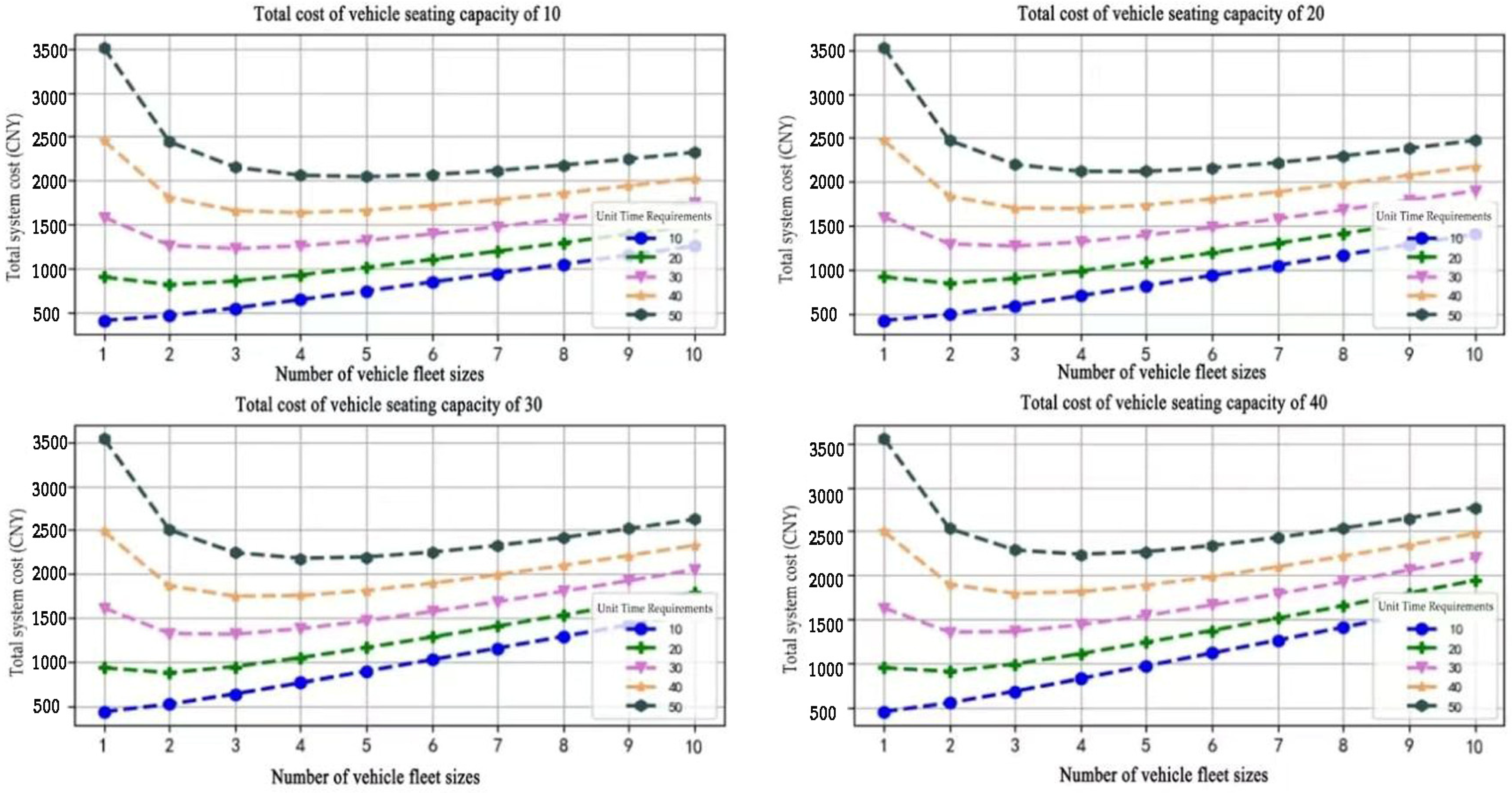
4.3. Impact of Different Fleet Sizes on Operation

Different fleet sizes will have an impact on the DRC’s parameters, such as running distance, waiting time, and in-vehicle time, and the relationship between fleet size and the impact of these parameters is further analyzed through simulation.

4.3.1. Traveling Distance

The influence of fleet size and demand density on travelling distance is shown in

Table 6. Numerical simulation results of DRC vehicle travel distance.

B	Q
	10	20	30	40	50
1	30.34	39.92	48.97	57.87	66.71
2	24.51	30.34	35.26	39.92	44.47
3	21.81	26.67	30.34	33.67	36.84
4	20.00	24.51	27.64	30.34	32.85
5	18.63	22.99	25.84	28.21	30.34
6	17.52	21.81	24.51	26.67	28.57

. For a given fleet size, the DRC traveling distance increases as the demand increases [44]. For a given level of demand, an increase in DRC fleet size results in a decrease in the overall diversions distance as well, and a decrease in the distance traveled by vehicles. As the number of vehicles operating increases from one to two vehicles/hour, the vehicle distance traveled decreases significantly, while the trend of decreasing distance traveled becomes flatter when the fleet size is larger than two vehicles/hour.

4.3.2. Average Waiting Time

The simulation results of fleet size and demand density on average waiting time are shown in

Table 7. Numerical simulation results of average waiting time.

B	Q
	10	20	30	40	50
1	0.80	1.02	1.24	1.46	1.68
2	0.69	0.80	0.91	1.02	1.13
3	0.66	0.73	0.80	0.88	0.95
4	0.64	0.69	0.75	0.80	0.86
5	0.63	0.67	0.71	0.76	0.80
6	0.62	0.66	0.69	0.73	0.77

. From the table, it can be seen that for a given fleet size, when travel demand increases, it means that the probability of a vehicle serving a newly requested stop increases, the route deviation distance increases, and the passenger waiting time increases. For a given level of demand, increasing fleet size results in an increase in the probability that a passenger with a new request for service will be accepted and a decrease in waiting time. When the fleet size is two to three vehicles/hour, an increase in demand density of 10 persons/hour increases the average waiting time by about 10 min, while when the vehicles exceed four vehicles/hour, the average waiting time increases by less than 3 min, suggesting that the right fleet size improves the operational efficiency, while continuing to increase the size reduces the waiting time insignificantly, but increases the overall operational cost.

4.3.3. Average In-Vehicle Time

The effects of travel demand and fleet size on average in-vehicle time are shown in

Table 8. Numerical simulation results of average in-train time.

B	Q
	10	20	30	40	50
1	0.53	0.68	0.83	0.97	1.12
2	0.46	0.53	0.61	0.68	0.75
3	0.44	0.49	0.53	0.58	0.63
4	0.43	0.46	0.50	0.53	0.57
5	0.42	0.45	0.48	0.51	0.53
6	0.41	0.44	0.46	0.49	0.51

. The change rule of average in-vehicle time and average waiting time is basically the same. Under a certain fleet size, as the demand density increases, the average in-vehicle time increases; while under a certain demand density, as the fleet size increases, the average in-vehicle time decreases; when the fleet size is larger than four vehicles/hour, the time decreases more gently.

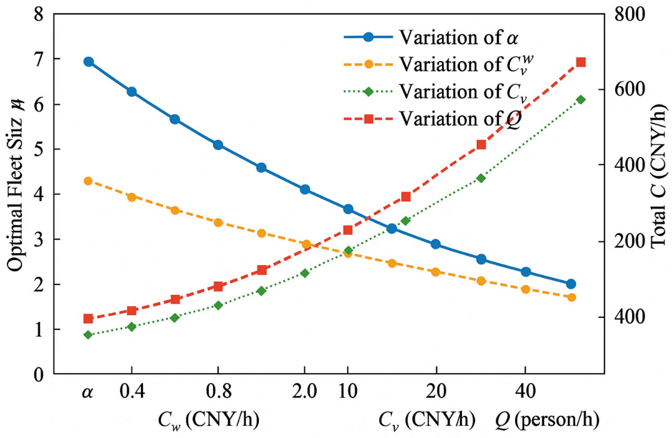
4.4. Analysis of Key Influencing Factors

In order to further study the variables affecting the optimal fleet size, this Section simulates the fleet size, demand density and DRC total system cost for different vehicle types, and seeks the relationship between fleet size and total system cost under different vehicle types and different demand densities, and it is not difficult to find out that there exists a minimum total system cost under different demand densities, and the fleet size corresponding to the minimum cost is the optimal fleet size [45]. The fleet size corresponding to the minimum cost is the optimal fleet size, and the optimal fleet size changes with the change in demand density and vehicle capacity. The change trend is shown in Figure 4.

Based on the above research, in order to further analyze the relationship between the key influencing factors in the DRC optimal fleet size model, obtain the optimal fleet size and the minimum cost value of the system under different vehicle capacities and different demand densities, and analyze the relationship between the vehicle capacities, demand densities, fleet sizes, and the total system costs. The specific simulation results are shown in

Table 9. Analysis of key impact factor results.

Q	k = 10		k = 20		k = 30		k = 40
	B	minC	B	minC	B	minC	B	minC
10	0.96	408.68	0.89	409.18	0.84	410.39	0.80	411.98
20	1.92	916.42	1.79	937.76	1.69	958.73	1.60	978.00
30	2.88	1620.98	2.69	1677.04	2.53	1730.93	2.39	1779.64
40	3.83	2522.29	3.58	2626.96	3.37	2726.92	3.19	2816.86
50	4.79	3620.34	4.47	3787.51	4.21	3946.70	3.99	4089.65

.

The results show that there is a certain linear relationship between the demand density and the optimal departure size under different vehicle capacities. When k = 10 seats/vehicle, the optimal fleet size is 0.096 times the density demand; when k = 20 seats/vehicle, the optimal fleet size is 0.089 times the density demand; when k = 30 seats/vehicle, the optimal fleet size is 0.084 times the density demand; when k = 40 seats/vehicle, the optimal fleet size is 0.080 times the density demand.

4.5. Case Illustration: Application Scenario in a City Fringe of Heilongjiang

To demonstrate the practical applicability of the proposed model, a case scenario based on an urban fringe area in Heilongjiang Province is introduced. This region exhibits sparse travel demand and limited conventional bus coverage, especially in suburban residential areas. The average demand density in this area is approximately 15 persons/h/km², mainly during morning and evening peak hours. The primary goal is to connect three residential communities to a major transit hub with trunk bus or metro services. Based on data from local transportation planning agencies, the proposed model is applied to determine optimal fleet size and departure frequency.

Simulation results show that the connector-type DRC can reduce total system cost by approximately 20% compared to fixed-route buses while maintaining passenger transfer waiting times below 0.7 h. Although no actual deployment has yet occurred, the operational parameters used are derived from real planning data, confirming the model’s practical relevance and feasibility.

4.6. Comparison of Different DRC

To better highlight the advantages and application scenarios of the connector-type demand-responsive connector (DRC) proposed in this study, we compare it with three other commonly used DRC models: order-based bus, dial-a-ride, and microtransit. The comparison is summarized in

Table 10. Comparison of different DRC.

Mode Type	Key Features	Advantages	Limitations	Suitable Scenarios
order-bus	Passengers reserve departure time and stop in advance	Reduces idle operation	Poor responsiveness	Medium- to low-density areas with regular commuting demand
dial-a-ride,	Passengers request door-to-door service via phone or app	High flexibility	High dispatching cost	Medical trips, elderly communities, small zones
microtransit	Small vehicles with flexible routing; complements transit	Urban supplement to conventional transit	Limited capacity	Urban sub-centers and transit hub catchment areas
Connector-Type DRC	Real-time response	Flexible service	Requires well-planned transfer points and smart routing	Urban fringes and suburban areas connecting to trunk lines

.

5. Conclusions

In this paper, based on the operating characteristics of DRC, the parameter models of passenger waiting time, vehicle operating cycle and passenger in-vehicle time are theoretically derived, and the fleet size optimization model is constructed with the objective of minimizing time cost and operating cost. The influence of travel demand and vehicle type on fleet size and total cost is analyzed through simulation, and on this basis, the influence law of fleet size, vehicle capacity type and demand density on passenger average waiting time, average in-vehicle time and vehicle travel distance is analyzed.

The results show that passenger average waiting time, average in-vehicle time, and vehicle travel distance all increase with the increase in demand density, and decrease with the increase in fleet size. When using single-vehicle or double-vehicle operation, the average waiting time, average in-vehicle time, and vehicle travel distance all decrease significantly with the increase in fleet size; when the fleet size is larger than two/vehicles, the average waiting time, average in-vehicle time, and vehicle travel distance gradually tends to level off. The decline gradually levelled off.

The primary contributions of this study are as follows:

• The study introduces a hybrid optimization approach that integrates both user costs and operational costs, offering an enhancement over traditional fleet allocation strategies, which typically consider only a single perspective.
• The study reveals a linear relationship between the optimal fleet size and demand density, while also examining the effect of vehicle capacity variations on this relationship. These findings possess notable generality and practical applicability.
• The developed model is highly adaptable to various operational scenarios and serves as an effective decision support tool for Demand-Responsive Transit (DRT) systems. It provides quantitative insights that can assist public transportation operators and urban transportation planners in formulating effective scheduling strategies.

Future research could incorporate real-world traffic networks and dynamic demand data to extend the model’s structure. This would involve considering the integration of multiple vehicle types and the implementation of spatiotemporal scheduling mechanisms. Additionally, exploring data-driven optimization methods could enhance the model’s feasibility and intelligence in practical systems.

In summary, the research in this paper provides a useful exploration of the scheduling and planning of demand response bus services in terms of theory and methodology, and lays the foundation for the realization of an efficient, low-cost, and high-service-level public transportation system.

References

1. Jokinen, J. Why urban mass demand responsive transport? In Proceedings of the 2011 IEEE Forum on Integrated and Sustainable Transportation Systems, Vienna, Austria, 29 June–1 July 2011; pp. 317–322. [Google Scholar]
2. Balac, M. Fleet Sizing for Pooled (Automated) Vehicle Fleets. Transp. Res. Rec. 2020, 2674, 168–176. [Google Scholar] [CrossRef]
3. Leich, G.; Bischoff, J. Should autonomous shared taxis replace buses? A simulation study. Transp. Res. Proc. 2019, 41, 450–460. [Google Scholar] [CrossRef]
4. Khanal, M. Estimating Demand for a New Travel Mode in Boise, Idaho. Sustainability 2021, 13, 1209. [Google Scholar] [CrossRef]
5. Ambrosino, G.; Nelson, J.; Romanazzo, M. Demand Responsive Transport Services: Towards the Flexible Mobility Agency; ENEA, Italian National Agency for New Technologies, Energy and the Sustainable Economic Development: Stockholm, Sweden, 2004. [Google Scholar]
6. Avermann, N.; Schlüter, J. Determinants of Customer Satisfaction with a True Door-To-Door Drt Service in Rural Germany. Res. Transp. Bus. Manag. 2019, 32, 100420. [Google Scholar] [CrossRef]
7. Berg, J.; Ihlstrom, J. The importance of public transport for mobility and everyday activities among rural residents. Soc. Sci. 2019, 8, 58. [Google Scholar] [CrossRef]
8. Boarnet, M.G.; Giuliano, G.; Hou, Y.; Shin, E.J. First/last mile transit access as an equity planning issue. Transp. Res. Pol. Pract. 2017, 103, 296–310. [Google Scholar] [CrossRef]
9. Noussan, M.; Tagliapietra, S. The effect of digitalization in the energy consumption of passenger transport: An analysis of future scenarios for Europe. J. Clean. Prod. 2020, 258, 120926. [Google Scholar] [CrossRef]
10. Gkiotsalitis, K.; Cats, O. Public transport planning adaption under the COVID-19 pandemic crisis: Literature review of research needs and directions. Transp. Rev. 2021, 41, 374–392. [Google Scholar] [CrossRef]
11. Storme, T.; De Vos, J.; Paepe, L.D.; Witlox, F. Limitations to the car-substitution effect of MaaS. Findings from a Belgian pilot study. Transp. Res. Part A Policy Pract. 2020, 131, 196–205. [Google Scholar] [CrossRef]
12. Clewlow, R.R.; Mishra, G.S. Disruptive Transportation: The Adoption, Utilization and Impacts of Ride-Hailing in the United States; Research Report UCD-ITS-RR-17-07; University of California. Institute of Transportation Studies: Davis, CA, USA, 2017. [Google Scholar]
13. Davison, L.; Enoch, M.; Ryley, T.; Quddus, M.; Wang, C. Identifying potential market niches for demand responsive transport. Res. Transp. Bus. Manag. 2012, 3, 50–61. [Google Scholar] [CrossRef]
14. Oldfield, R.H.; Bly, P.H. An analytic investigation of optimal bus size. Transp. Res. Part B Methodol. 1988, 22, 319–337. [Google Scholar] [CrossRef]
15. Yang, H.; Cherry, C.R.; Zaretzki, R.; Ryerson, M.S.; Liu, X.; Fu, Z. A GIS-based method to identify cost-effective routes for rural deviated fixed route transit. J. Adv. Transp. 2016, 50, 1770–1784. [Google Scholar] [CrossRef]
16. Ciaffi, F.; Cipriani, E.; Petrelli, M. Feeder bus network design problem: A new Metaheuristic procedure and real size applications. Procedia-Soc. Behav. Sci. 2012, 54, 798–807. [Google Scholar] [CrossRef]
17. Burris, M.; Pendyala, R. Discrete choice models of traveler participation in difierential time of day pricing programs. J. Transp. Policy 2002, 9, 241–251. [Google Scholar] [CrossRef]
18. Kaddoura, I.; Kickhöfer, B.; Neumann, A.; Tirachini, A. Optimal public transport pricing: Towards an agent-based marginalsocial cost approach. J. Transp. Econ. Policy 2015, 49, 200–218. [Google Scholar]
19. Roson, R. Social cost pricing when public transport is an option value. Innov. Eur. J. Soc. Sci. Res. 2000, 13, 81–94. [Google Scholar] [CrossRef]
20. Qiu, C.; Yan, H.; Li, N.; Li, T. The optimal design of Beijing bus fares of transit system. Res. Appl. Econ. 2014, 2, 72–79. [Google Scholar]
21. Szeto, W.; Wu, Y. A simultaneous bus route design and frequeney setting problem for Tin Shui Wai, Hong Kong. Eur. J. Oper. Res. 2011, 209, 141–155. [Google Scholar] [CrossRef]
22. Zeng, Y.Z.; Ran, B.; Zhang, N.; Yang, X.; Shen, J.J.; Deng, S.J. Optimal pricing and service for the peak-period bus commuting inelicieney of boarding queuing congestion. Sustainability 2018, 10, 3497. [Google Scholar] [CrossRef]
23. Wagale, M.; Singh, A.P.; Sarkar, A.K.; Arkatkar, S. Real-time optimal bus scheduling for a city using A DTR model. Procedia-Soc. Behav. Sci. 2013, 104, 845–854. [Google Scholar] [CrossRef]
24. Avila, P.; lrarragorri, F.; Caballero, R. A bi-objective model for the integrated frequency-timetabling problem. J. WIT Trans. Built Environ. 2014, 138, 209–219. [Google Scholar]
25. Huang, Z.; Gang, R.; Liu, H. Optimizing bus frequencies under uncertain demand: Case study of the transit network in a developing city. Math. Probl. Eng. 2013, 2013, 375084. [Google Scholar] [CrossRef]
26. Li, X.; Liao, J.; Wang, T.; Lu, L. Integrated optimization of bus bridging route design and bus resource allocation in response to metro service disruptions. J. Transp. Eng. Part A Syst. 2022, 148, 04022050. [Google Scholar] [CrossRef]
27. Wang, Y.; Chen, J.; Liu, Z. Terminal-based zonal bus: A novel flexible transit system design and implementation. Expert Syst. Appl. 2024, 238, 121793. [Google Scholar] [CrossRef]
28. Emami, B.D.; Zhang, Y.; Khani, A.; Song, Y. Towards an efficient electric bus system: Multi-phase optimization model for incremental electrification of bus network with uncertain energy consumption. Transp. Res. Part C Emerg. Technol. 2025, 173, 105011. [Google Scholar] [CrossRef]
29. Yetkin, M.; Augustino, B.; Lamadrid, A.J.; Snyder, L.V. Co-optimizing the smart grid and electric public transit bus system. Optim. Eng. 2024, 25, 2425–2472. [Google Scholar] [CrossRef]
30. Zhu, Y.; Wang, H. Path-choice-constrained bus bridging design under urban rail transit disruptions. Transp. Res. Part E Logist. Transp. Rev. 2024, 188, 103637. [Google Scholar] [CrossRef]
31. Golbabaei, F.; Yigitcanlar, T.; Paz, A.; Bunker, J. Understanding Autonomous Shuttle Adoption Intention: Predictive Power of Pre-Trial Perceptions and Attitudes. Sensors 2022, 22, 9193. [Google Scholar] [CrossRef]
32. Qu, B.; Mao, L.; Xu, Z.; Feng, J.; Wang, X. How Many Vehicles Do We Need? Fleet Sizing for Shared Autonomous Vehicles with Ridesharing. IEEE Trans. Intell. Transp. Syst. 2022, 23, 14594–14607. [Google Scholar] [CrossRef]
33. Winter, K.; Cats, O.; Correia, G.H.D.; van Arem, B. Designing an Automated Demand-Responsive Transport System Fleet Size and Performance Analysis for a Campus-Train Station Service. Transp. Res. Rec. 2016, 2542, 75–83. [Google Scholar] [CrossRef]
34. Quadrifoglio, L.; Dessouky, M. Insertion heuristic for scheduling mobility allowance shuttle transit services: Sensitivity to service area. In Computer-Aided Systems in Public Transport; Springer Series: Lecture Notes in Economics and Mathematical Systems; Springer: Berlin/Heidelberg, Germany, 2007; Volume 600, pp. 419–437. [Google Scholar]
35. Quadrifoglio, L.; Dessouky, M. Sensitivity analyses over the service area for mobility allowance shuttle transit (MAST) services. In Computer-Aided Systems in Public Transport; Springer: Berlin/Heidelberg, Germany, 2018; Volume 600, pp. 419–432. [Google Scholar]
36. Kim, M.E.; Schonfeld, P.; Kim, E. Switching service types for multi-region bus systems. Transp. Plan. Technol. 2018, 41, 617–643. [Google Scholar] [CrossRef]
37. Takeuchi, R.; Okura, I.; Nakamura, F.; Hiraishi, H. Feasibility Study on Demand Responsive Transport Systems (Drts). In Proceedings of the 5th Eastern Asia Society for Transportation Studies Conference, Hokkaido, Japan, 12 November 2003. [Google Scholar]
38. Velaga, N.R.; Beecroft, M.; Nelson, J.D.; Corsar, D.; Edwards, P. Transport poverty meets the digital divide: Accessibility and connectivity in rural communities. J. Transp. Geogr. 2012, 21, 102–112. [Google Scholar] [CrossRef]
39. Liu, Z.; Shen, J. Regional bus operation bi-level programming model integrating timetabling and vehicle scheduling. Syst. Eng.-Theory Pract. 2007, 27, 135–141. [Google Scholar] [CrossRef]
40. Yu, H.; Mu, D. Carbon Emission Research of Beijing Transportation System Based on SD. In Proceedings of the 2016 International Conference on Logistics, Informatics and Service Sciences (LISS), Sydney, Australia, 24–27 July 2016; pp. 1–4. [Google Scholar]
41. Wang, L.; Fan, J.; Wang, J.; Zhao, Y.; Li, Z.; Guo, R. Spatio-Temporal Characteristics of the Relationship between Carbon Emissions and Economic Growth in China’s Transportation Industry. Environ. Sci. Pollut. Res. 2020, 27, 32962–32979. [Google Scholar] [CrossRef] [PubMed]
42. Shan, Y.; Guan, D.; Zheng, H.; Ou, J.; Li, Y.; Meng, J.; Mi, Z.; Liu, Z.; Zhang, Q. China CO2 Emission Accounts 1997–2015. Sci. Data 2018, 5, 1–14. [Google Scholar] [CrossRef]
43. Pan, X.; Wei, Z.; Han, B.; Shahbaz, M. The Heterogeneous Impacts of Interregional Green Technology Spillover on Energy Intensity in China. Energy Econ. 2021, 96, 105133. [Google Scholar] [CrossRef]
44. Yang, Y.; Yan, F. An Inquiry into the Characteristics of Carbon Emissions in Inter-Provincial Transportation in China: Aiming to Typological Strategies for Carbon Reduction in Regional Transportation. Land 2024, 13, 15. [Google Scholar] [CrossRef]
45. Wang, D.; Han, B. Effects of Indigenous R&D and Foreign Spillover on Energy Intensity in China. J. Renew. Sustain. Energy 2017, 9, 035901. [Google Scholar]
Figure 1. DRC operating mode.
Applsci 15 05350 g001
Figure 2. Algorithm diagram of cost model of DRC and cost-based fleet size model.
Applsci 15 05350 g002
Figure 3. Virtual simulation results curve diagram.
Applsci 15 05350 g003
Figure 4. Trends in optimal fleet size under different scenarios.
Applsci 15 05350 g004