Kriging-Based Time-Variant Reliability Analysis Incorporating Error Distance Function and First Crossing Time Point

Abstract

To address the time-variant reliability (TVR) issue during a structure’s life cycle, we propose an innovative Kriging method named EDFK-FCTP. This active-learning TVR analysis is based on an error distance function (EDF) and the first crossing time point (FCTP). We employ Latinized partially stratified sampling (LPSS) to estimate the first four-order origin moments of the FCTP surrogate model. The convergence condition for establishing the optimal surrogate model for the FCTP is determined by the geometric mean of the probability density of training samples and the maximum error of the first four-order origin moments across two adjacent iterations. Utilizing the optimal surrogate model, the probability density function (PDF) of the FCTP is solved using kernel density estimation (KDE), thereby deriving the failure probability of the structure throughout its life cycle. Example analyses demonstrate that the calculation accuracy of our proposed method fulfills engineering requirements. Notably, it presents certain advantages over alternative methods, particularly in regions of low failure probability. For complex performance functions, our method offers significant computational efficiency benefits compared to other approaches.

1. Introduction

The reliability of mechanical structures is of great significance in enhancing the stability of products. Based on traditional time-invariant reliability models, the degradation phenomena of internal materials are usually not considered, and the calculated structural reliability is a constant value. The complexity and intelligence of the mechanical system give the system performance obvious time-variant dynamic characteristics. Complex engineering requirements cannot be met through traditional static reliability analysis methods. However, temporal variables, spatial variables, and the correlation of structural performance between time points are considered in time-variant reliability (TVR) analysis methods. Trends in the reliability of the system over the life cycle can be reflected to some extent [1,2].

The main approaches to solving TVR structural problems are the approximate analytical method [3,4], the numerical simulation method [5,6], and the surrogate model method [7,8]. Jiang et al. [9,10] discretized stochastic processes, and the TVR problem was transformed into a traditional time-invariant reliability problem. However, the accuracy and efficiency are seriously affected by the size of discrete time intervals. To address this limitation, Zhang et al. [11] applied the Kriging surrogate model to approximate the trajectory of the maximum possible point (MPP), referred to as AMPPT. Zhang et al. [12] improved training efficiency by applying the active Kriging surrogate model to the traditional stochastic process discretization method. Meng et al. [4] proposed a semi-analytic extreme value method to approximate the limit state function (LSF) at the MPP. However, searching for the MPP requires calling a large number of time-variant LSF, which is less efficient.

Meanwhile, the method cannot address multiple MPPs or highly nonlinear and complex LSFs. Wu et al. [13] proposed a system reliability method by combining the envelope method and the second-order reliability method (SORM). Gong and Frangopol [14] proposed a new method for analyzing TVR based on the first-order reliability method (FORM). In addition, Wang and Chen [15] proposed a stochastic process transformation method considering both random variables and stochastic process parameters for solving whole life cycle reliability variation.

The main numerical simulation methods are Monte Carlo Simulation (MCS) [16], Subset Simulation (SS) [17], and Importance Sampling (IS) [6], etc. The advantages of the numerical simulation method are high accuracy and simple operation. Moreover, the dimensionality problem and complexity of LSF need not be taken into account. However, the guarantee of computational accuracy requires a large number of samples, which leads to inefficient computation [18].

The surrogate model method approximates the actual model by constructing a function and applies the constructed function to solve TVR, which greatly improves computational efficiency. Hu et al. [19] proposed an effective TVR analysis method based on a fast integration approach and surrogate model method. Classical approaches include the double-loop approach [20,21] and the single-loop approach. Wang et al. [22] proposed a coupled extreme value response surface method based on double-loop substitution. Hu and Du [21] improved the coupled extreme value response surface method to construct a more efficient adaptive Kriging–MCS hybrid model. The method based on a double-loop surrogate model needs to find extreme value in the inner loop and use the result to perform reliability analyses in the outer loop, which is inefficient. In order to improve efficiency, the single-loop method is proposed to transform the TVR problem into a classification problem through the adaptive surrogate model, e.g., single-loop Kriging (SILK) [23,24]. With the surrogate model method, high nonlinearities, high dimensionality, and implicit performance functions can be handled well. However, only reliability over a particular time interval can be obtained. Solving the trend of reliability over the whole life cycle of a product requires discretizing the life cycle and calculating the reliability in different time intervals, which is inefficient [18].

Among the TVR methods based on the crossing rate, Rice [25] pioneered the first crossing rate theory to study the problem of dynamic response exceeding a certain fixed threshold at a given time, laying the foundation for the development of the first crossing rate method. Andrieu-Renaud et al. [3] proposed the PHI2 method to convert the time-variant problem into a static parallel system reliability problem, improving the efficiency greatly. To address the lack of stability of the PHI2 method, Sudret et al. [26] proposed the PHI2+ method with a more concise process for the calculation of the crossing rate. Hu et al. [27] proposed the Rice/FORM to solve the TVR of the structure by converting the time-variant performance function to the Gaussian process to calculate the crossing rate. Jiang et al. [28] converted the calculation of the crossing rate in the time-variant system into a solution of reliability in the time-invariant system, improving the efficiency of the solution. Although the crossing rate approach is effective in solving TVR problems, there are some inherent drawbacks, such as the assumption of Poisson distribution of crossing events and the limitations imposed by the application of FORM.

In this paper, a first crossing approach for analyzing TVR based on the error distance function (EDF) and Kriging surrogate model is presented, referred to as EDFK-FCTP. The EDFK-FCTP method establishes the functional relationship between the first crossing time point (FCTP) and input random variables by constructing the adaptive Kriging model. Moreover, kernel density estimation (KDE) is used to estimate the probability density function (PDF) of the FCTP, eliminating the probabilistic assumptions of traditional crossing rate methods. Hence, in this paper, (1) a Kriging-based adaptive surrogate model of FCTP is developed; (2) the EDF is constructed by combining model error and sample distance; (3) the geometric mean of probability density of training samples and the maximum error of the first four order origin moments of two adjacent iterations are used as the convergence condition to establish the optimal surrogate model for FCTP; (4) on the basis of the optimal surrogate model, KDE is used to solve PDF of the FCTP to obtain trend of failure probability during the product life cycle.

2. TVR Problem

2.1. Problem Statement

TVR is the probability that a structure performs a specified function within a specified time, affected by time-variant uncertainties. Over the life cycle $[0,T]$, the failure probability $P_f\left(T\right)$ can be expressed as follows:

$$P_f\left(T\right)=P\left\{g(\mathit{X},\mathit{Y}(t),t)\le 0,\exists t\in [0,T]\right\}$$

(1)

where $P\{ \}$ denotes probability calculation; $g$ denotes LSF of structure; $\mathit{X}=\left[X_1,X_2,\dots ,X_n\right]$ is the vector of n-dimensional random variables; $\mathit{Y}\left(t\right)=\left[Y_1\left(t\right),Y_2\left(t\right),\dots ,Y_m\left(t\right)\right]$ is m-dimensional random process vector.

The prerequisite for solving the reliability of a product over the life cycle $[0,T]$ is to calculate reliability at each moment in time. Let $\tau$ be an arbitrary moment point in life cycle $[0,T]$. According to Equation (1), the failure probability at moment $\tau$ can be expressed as follows:

$$P_f\left(\tau \right)=P\left\{g(\mathit{X},\mathit{Y}(t),t)\le 0,\exists t\in [0,\tau ]\right\},0\le \tau \le T$$

(2)

In order to simplify the calculation process, the stochastic process $\mathit{Y}\left(t\right)$ is expressed as a coupled function of random variable ${\mathit{Y}}^{\mathit{*}}$ and time $t$ based on the stochastic process discretization method [29]. The LSF $g(\mathit{X},\mathit{Y}(t),t)$ is transformed into a function only with regard to random variables and time, where $\mathit{Z}=(\mathit{X},{\mathit{Y}}^{\mathit{*}})$. The failure probability of the product at moment $\tau$ can be finally expressed as follows:

$$P_f\left(\tau \right)=P\left\{g(\mathit{Z},t)\le 0,\exists t\in [0,\tau ]\right\},0\le \tau \le T$$

(3)

The reliability $P_r\left(\tau \right)$ of structure over the life cycle can be expressed as follows:

$$P_r\left(\tau \right)=P\left\{g(\mathit{Z},t)>0,\forall t\in [0,\tau ]\right\},0\le \tau \le T$$

(4)

2.2. Analysis Methods

Specific sample $\mathit{Z}$ is generated based on the probabilistic properties of input random variable $\mathit{Z}$. In the case of sample determination, the LSF can be viewed as a unitary function $g(\mathit{Z},t)$ only with regard to time $t$. The TVR analysis methods can be classified into extreme value method and FCTP method based on how Equations (3) and (4) are calculated.

The extreme value method considers whether the condition is satisfied for the minimum value of LSF response in the time interval $[0,\tau ]$. Hence, Equation (3) can be transformed as follows:

$$P_f(\tau )=P\left\{\underset{t\in [0,\tau ]}{min}g(\mathit{Z},t)\le 0\right\},0\le \tau \le T$$

(5)

The FCTP considers the location relationship between time interval $[0,\tau ]$ and moment point of unitary function $g(Z,t)$ from safety domain to failure domain based on specific samples. As shown in Figure 1, there are three intersection points between $g(Z,t)$ and the time axis, $t_1$, $t_2$, and $t_3$, defining $t_1$ as FCTP. Whether structure fails or not depends on the position relationship of $t_1$ and the time interval $[0,\tau ]$.

From the structure of the function of $g(\mathit{Z},t)$, sample points and FCTPs correspond to each other.

TP $t_1$ is function of the input random variable $\mathit{Z}$, denoted $ct=\phi \left(\mathit{Z}\right)$. The failure probability of structure in the time interval $[0,\tau ]$ can be expressed as follows:

$$P_f\left(\tau \right)=P\left\{0\le ct\le \tau \right\}$$

(6)

For Equation (6), the LSF can be transformed to be solved. As shown in Figure 2, the two curves and gray shaded portions contained represent all possible performance functions, i.e., clusters of performance functions. The first intersection of the cluster of performance functions with time axis constitutes the FCTP set. The set can be represented as a function of input variables, i.e., $ct=\phi \left(\mathit{Z}\right)$. The black shaded portion can represent the PDF of FCTP, $f\left(\omega \right)$. Equation (6) can be transformed as follows:

$$P_f(\tau )={\int }_0^{\tau }f\left(\omega \right)d\omega$$

(7)

Traditional methods of calculating crossing rates need to be based on certain assumptions about stochastic processes. However, the assumptions remain somewhat controversial. And the methods can only be used for a few special forms of performance functions. The MCS method is highly inefficient in calculating crossing rates. Therefore, in this paper, a novel TVR analysis method [30] is used to calculate the failure probability of structure.

3. Kriging-Based Probability Density Estimation for FCTP

For LSF with high dimensionality and high nonlinearity, MCS-based methods for solving FCTP using $g(\mathit{Z},t)=0$ is inefficient. In this paper, the FCTP surrogate model based on the origin moment estimation method combining Latinized partially stratified sampling (LPSS) [31] and the adaptive Kriging model [32] is constructed. KDE solves the PDF of FCTP.

3.1. Kriging Model

The Kriging surrogate model is an unbiased estimation model [33] that combines global approximation with local random errors to fit highly nonlinear models well. The Kriging surrogate model represents the response value as a combination of a parameterized polynomial model and a non-parameterized stochastic process [32], which is generally expressed as follows:

$$y\left(\mathit{x}\right)\approx y_K\left(\mathit{x}\right)=G^T\left(\mathit{x}\right)\mathit{\beta }+z\left(\mathit{x}\right)$$

(8)

where $y\left(\mathit{x}\right)$ is true model, $y_K\left(\mathit{x}\right)$ is the pending Kriging model, $\mathit{G}\left(x\right)={\left[G_1\left(\mathit{x}\right),G_2\left(\mathit{x}\right),\dots ,G_k\left(\mathit{x}\right)\right]}^T$ is the matrix of basis functions, $k$ is the number of basis functions, $\mathit{\beta }={\left[{\beta }_1,{\beta }_2,\dots ,{\beta }_k\right]}^T$ is matrix of unknown weight coefficients, which can be estimated from the training samples, ${\mathit{G}}^T\left(\mathit{x}\right)\mathit{\beta }$ denotes parameterized polynomial model, which gives trend of the model, and $z\left(\mathit{x}\right)$ denotes a non-parametrizable stochastic process, which provides information about deviation of the model, the probabilistic properties are as follows:

$$\left\{\begin{array}{c}E\left(z\right(\mathit{x}\left)\right)=0\\ Var\left(z\right(\mathit{x}\left)\right)={\sigma }_z^2\\ Cov\left[z\left({\mathit{x}}_i\right),z\left({\mathit{x}}_j\right)\right]={\sigma }_z^2\left[R\left(\theta ,{\mathit{x}}_i,{\mathit{x}}_j\right)\right]\end{array}\right.$$

(9)

where ${\sigma }_z^2$ is the random process variance, and $\theta$ is the correlation parameter to be sought.

Assuming that there are $p$ training samples $\left\{{\mathit{x}}_i:i=\mathrm{1,2},\dots ,p\right\}$, the correlation matrix between the samples is denoted as follows:

$$\mathit{R}=\left[\begin{array}{cccc}R({\mathit{x}}_1,{\mathit{x}}_1)& R({\mathit{x}}_1,{\mathit{x}}_2)& \dots & R({\mathit{x}}_1,{\mathit{x}}_p)\\ R({\mathit{x}}_2,{\mathit{x}}_1)& R({\mathit{x}}_2,{\mathit{x}}_2)& \dots & R({\mathit{x}}_2,{\mathit{x}}_p)\\ ⋮& ⋮& \ddots & ⋮\\ R({\mathit{x}}_p,{\mathit{x}}_1)& R({\mathit{x}}_p,{\mathit{x}}_1)& \dots & R({\mathit{x}}_p,{\mathit{x}}_p)\end{array}\right]$$

(10)

For prediction point $\mathit{x}$, the correlation vector is

$$r\left(\mathit{x}\right)=\left[R({\mathit{x}}_1,\mathit{x}),R({\mathit{x}}_2,\mathit{x}),\dots ,R({\mathit{x}}_p,\mathit{x})\right]$$

(11)

After selecting the correlation function, according to the Kriging theory [34], the optimal unbiased prediction response of model can be expressed as follows:

$$y_K(\mathit{x})={\mathit{G}}^T(\mathit{x})\widehat{\mathit{\beta }}+{\mathit{r}}^T(\mathit{x}){\mathit{R}}^{-1}\left(\mathit{Y}-\mathit{g}\widehat{\mathit{\beta }}\right)$$

(12)

$$\widehat{\mathit{\beta }}={\left({\mathit{g}}^T{\mathit{R}}^{-1}\mathit{g}\right)}^{-1}\left({\mathit{g}}^T{\mathit{R}}^{-1}\mathit{Y}\right)$$

(13)

where $\widehat{\mathit{\beta }}$ is estimate of $\mathit{\beta }$, $\mathit{Y}$ is output value of the training samples, and $\mathit{g}$ is a matrix consisting of the values of $k$ basis functions at $p$ training samples. The variance estimate is expressed as follows:

$${\widehat{\sigma }}_z^2={\displaystyle \frac{{\left(\mathit{Y}-\mathit{g}\widehat{\mathit{\beta }}\right)}^T{\mathit{R}}^{-1}\left(\mathit{Y}-\mathit{g}\widehat{\mathit{\beta }}\right)}{p}}$$

(14)

If Gaussian function is chosen as the correlation function, the parameter vector $\mathit{\theta }$ can be solved by great likelihood estimation:

$$\mathit{max}W\left(\mathit{\theta }\right)=\left[-{\displaystyle \frac{p}{2}}{\mathit{ln}{\sigma }_z}^2-{\displaystyle \frac{1}{2}}\mathit{ln}|\mathit{R}|\right]$$

(15)

If any unknown random input variable and output response both obey Gaussian distribution, the mean ${\mu }_y\left(\mathit{x}\right)$ and variance ${\sigma }_y^2\left(\mathit{x}\right)$ are given by

$${\mu }_y\left(\mathit{x}\right)={\mathit{G}}^T\left(\mathit{x}\right)\widehat{\mathit{\beta }}+{\mathit{r}}^T\left(\mathit{x}\right){\mathit{R}}^{-1}\left(\mathit{Y}-\mathit{g}\widehat{\mathit{\beta }}\right)$$

(16)

$${\sigma }_y^2\left(\mathit{x}\right)={\sigma }_z^2{\left[{\mathit{g}}^T{\mathit{R}}^{-1}\mathit{r}\left(\mathit{x}\right)-\mathit{G}\left(\mathit{x}\right)\right]}^T{\left({\mathit{g}}^T{\mathit{R}}^{-1}\mathit{g}\right)}^{-1}\left[{\mathit{g}}^T{\mathit{R}}^{-1}\mathit{r}\left(\mathit{x}\right)-\mathit{G}\left(\mathit{x}\right)\right]+{\sigma }_z^2\left[1-{\mathit{r}}^T\left(\mathit{x}\right){\mathit{R}}^{-1}\mathit{r}\left(\mathit{x}\right)\right]$$

(17)

The values of ${\mu }_y\left(\mathit{x}\right)$ and ${\sigma }_y^2\left(\mathit{x}\right)$ were solved by the MATLAB (R2023a) toolbox UQLab [35]. At the training samples ${\mathit{x}}^{*}$, there are ${\mu }_y\left({\mathit{x}}^{*}\right)=y\left({\mathit{x}}^{*}\right)$ and ${\sigma }_y^2\left({\mathit{x}}^{\mathit{*}}\right)=0$. Generally, ${\sigma }_y^2\left(\mathit{x}\right)\ne 0$ at other samples. The degree of deviation of predicted value from actual value at $\mathit{x}$ can be reflected through ${\sigma }_y^2\left(\mathit{x}\right)$. Thus, ${\sigma }_y^2\left(\mathit{x}\right)$ is able to reflect the predictive accuracy of the surrogate model at $\mathit{x}$.

3.2. Initial Surrogate Model of FCTP

For initial training samples, various sampling methods are available, such as random sampling (RS), Latin hypercube sampling (LHS), and uniform sampling (US). At high dimensions, sample collection in significant space cannot be guaranteed using RS. LHS and US ensure that sampling points are as dispersed as possible. However, the stochastic properties of LHS method may lead to the instability of the surrogate model when the training samples are few. Therefore, in this paper, the US method is used to generate initial training samples. In addition, the transformation of all random variables involved in the reliability problem from the space to which they belong to standard normal space through Nataf transform [36] facilitates the computation. A larger sampling range is not only slow to converge, but fitting accuracy is also reduced, especially for nonlinear problems. Based on the $3\sigma$ principle, the initial sample range in standard normal space is determined as $[-\mathrm{3,3}]$, and the range is continuously reduced during the iteration process. According to Shi [37], the number of initial sampling points is generally 10~15 to ensure the accuracy of the model and the efficiency of active learning. Also, considering the effect of dimensionality determines the number of initial samples to be

$$N_0=\mathit{max}(2d+1.12)$$

(18)

where $d$ is the number of dimensions. The initial samples can be represented as follows:

$${\mathit{Z}}^{initial}=\left[\begin{array}{cccc}{z}_1^{\left(1\right)}& z_2^{\left(1\right)}& \cdots & z_d^{\left(1\right)}\\ z_1^{\left(2\right)}& z_2^{\left(2\right)}& \cdots & z_d^{\left(2\right)}\\ ⋮& ⋮& \ddots & ⋮\\ z_1^{N_0}& z_2^{N_0}& \cdots & z_d^{N_0}\end{array}\right]$$

(19)

It can also be expressed as:

$${\mathit{Z}}^{initial}={\left[{{\mathit{z}}_1}^{initial},{{\mathit{z}}_2}^{initial},\dots ,{{\mathit{z}}_{N_0}}^{initial}\right]}^T$$

(20)

where ${{\mathit{z}}_i}^{initial}=\left[z_i^1,z_i^2,\dots z_i^d\right]$, $i=\mathrm{1,2},\dots ,N_0$.

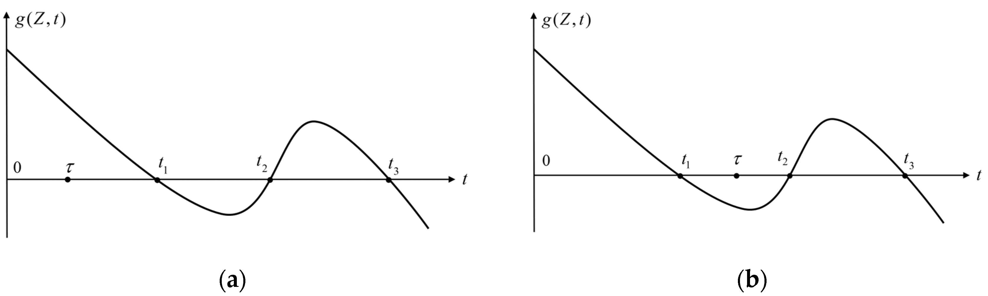
After generating the initial training sample ${{\mathit{z}}_i}^{initial}$, the performance function $g(\mathit{Z},t)$ can be viewed as univariate function $g\left({{\mathit{z}}_i}^{initial},t\right)$ of time. Thus, the FCTP $c{t_i}^{initial}$ of initial training sample can be solved by the following equation:

$$g\left({{\mathit{z}}_i}^{initial},t\right)=0$$

(21)

The initial set of training samples $\left\{{{\mathit{z}}_i}^{initial},c{t}_i^{initial}\right\}$, $i=\mathrm{1,2},\dots ,N_0$ is obtained. Further, the initial Kriging surrogate model of FCTP is constructed using Equation (8). The subsequent jth iteration is denoted ${\widehat{\phi }}^{\left(j\right)}(\mathit{Z})$.

3.3. Active Learning Function EDF

After transforming input random variables into mutually independent standard normal variables [38], the first-order origin moments of the jth FCTP surrogate model can be expressed as follows:

$$M_l^{\left(j\right)}=\int \cdots {\int }_{-\infty }^{+\infty }{\left[{\widehat{\phi }}^{\left(j\right)}(\mathit{Z})\right]}^l\varphi (\mathit{Z})d\mathit{Z}$$

(22)

where $\varphi \left(\mathit{Z}\right)$ is the joint probability density function of mutually independent standard normal distributions. Since most of the integrated functions composed of LSF and PDF are not integrable [39], numerical methods can be used to approximate the integration process of Equation (22):

$$M_l^{\left(j\right)}\approx {\sum _{j=1}^a{\lambda }_j\left[{\widehat{\phi }}^{\left(j\right)}\left({\vartheta }_j\right)\right]}^l$$

(23)

where ${\vartheta }_j$ is the integration point of numerical integration, ${\lambda }_j$ is the weight coefficient corresponding to the integration point, and $a$ is the number of integration points. In this paper, the LPSS method is used to generate the integration points and weight coefficients.

The key to efficient surrogate modeling lies in the sample selection strategy [40]. This paper summarizes two main factors influencing sample selection:

(1) Model Error. The mean can measure the model error, variance, and joint PDF [41]. Since the first-order origin moments characterize the mean value, the samples selected should be generated as close as possible to the mean of FCTP. The approximate first-order origin moments of the jth FCTP surrogate model $M_1^{\left(j\right)}$ can be obtained using Equation (23). Variance measures the degree of dispersion of the data and is an important basis for constructing active learning methods. The variance estimate of the Kriging surrogate model can be obtained by Equation (17), characterizing the prediction error of the model at the prediction point. The joint PDF $f\left(x\right)$ of random variables can ensure that the selected points fall in a large probability region, effectively improving the estimation accuracy of the model.

(2) Sample Distance. The distance between samples is an important principle in sample selection. On the one hand, the selected samples should be as sparse as possible to ensure global accuracy of the model; on the other hand, the selected samples should be prevented from bunching to avoid reducing the utilization rate of samples. In the $s$ dimensional space $R^s$, the Euclidean distance $d_a$ from any point $x$ to point $x_a$ is

$$d_a=\sqrt{\sum _{i=1}^s{\left(x^{\left(i\right)}-x_a^{\left(i\right)}\right)}^2}$$

(24)

It is assumed that current surrogate model training set $\xi$ has $n_{\xi }$ sample points $x_c\in \xi$, $c=\mathrm{1,2},\dots ,n_{\xi }$, The distance from any point $x$ to each point in set $\xi$ is

$$d_{\xi }(x)=\left\{d_1(x),d_2(x),\dots ,d_{n_{\xi }}(x)\right\}$$

(25)

The average value $\overline{d_{\xi }\left(x\right)}$ of distances from point $x$ to each point in set $\xi$ can be used as a measure of the sparsity of the samples:

$$\overline{d_{\xi }\left(x\right)}={\displaystyle \frac{{\sum }_{c=1}^{n_{\xi }}{d}_c\left(x\right)}{n_{\xi }}}$$

(26)

Using the minimum distance $d_m\left(x\right)$ from any point $x$ to each point in set $\xi$ can avoid bunching as follows:

$${d_m\left(x\right)=\mathit{min}\left(d_{\xi }\left(x\right)\right)}_m$$

(27)

It is essential to choose a suitable active learning function for building highly accurate and efficient surrogate models. Too many adaptive selected samples can consume a lot of computational resources and reduce the benefits of the surrogate model method. Model accuracy cannot be guaranteed with too few samples. Based on the above two major factors, the active learning function EDF is proposed with the following expression:

$$EDF(x)=(1-\alpha ){\displaystyle \frac{\mathit{max}\left(\widehat{\sigma }(x)\right)\left|M_1^{(j)}-{\phi }^{)j)})x)\right|}{\widehat{\sigma }(x)f(x)\mathit{max}\left(\left|M_1^{(j)}-{\phi }^{(j)}(x)\right|\right)}}+\alpha {\displaystyle \frac{\mathit{max}\left(d_m(x)\right)\mathit{max}\left(\overline{d_{\xi }(x)}\right)}{d_m(x)\overline{d_{\xi }(x)}}}$$

(28)

where $\alpha \in \left(\mathrm{0,1}\right)$ is the weight coefficient, $\alpha =0.5$ in this paper. The difference $\alpha$ characterizes the importance of model error with sample distance and contribution to the learning function. On the composition of the EDF, the relationship between $\mathit{max}\left(\mathrm{*}\right)$ and $\mathrm{*}$ is very important. The ratio of $\mathit{max}\left(\mathrm{*}\right)$ and $\mathrm{*}$ is a dimensionless number, which reflects the degree of approximation of the selected point to the ideal model. The EDF involves $\mathrm{*}$ with $\widehat{\sigma }(x)$, $\left|M_1^{\left(j\right)}-{\phi }^{\left(j\right)}(x)\right|$, $d_m(x)$ and $\overline{d_{\xi }(x)}$, where $\left|M_1^{\left(j\right)}-{\phi }^{\left(j\right)}(x)\right|$ means that the selected sample points should be generated as close as possible to the mean value of the FCTP. At the same time, the influence of probability density function and variance is considered.

Further, in the pool of possible samples ${\Omega }^s$, the point that minimizes the learning function $EDF\left(x\right)$ will be selected as the new central sample as follows:

$$x_{new}=\mathit{arg}\underset{x\in {\Omega }^s}{min}(EDF(x))$$

(29)

Based on the $3\sigma$ principle, $N_0$ initial training samples are generated in the range $[-3,3]$ to improve the convergence rate of the model. $d+1$ samples are added uniformly to the training sample set on the hypersphere centered at $x_{new}$ with radius $r$ in subsequent iterations. Moreover, the sample interval $r$ decreases gradually:

$$r_j=\left\{\begin{array}{c}2,j=1\\ 0.5r_{j-1},j\ge 2\end{array}\right.$$

(30)

Convergence conditions need to be set to ensure model accuracy. The geometric mean of the probability density of training samples and the maximum error of the first four order origin moments of two adjacent iterations are taken as the convergence conditions. The specific mathematical expression is

$$1-\sqrt{f^{\left(j\right)}(x)f^{(j-1)}(x)}<{\varsigma }_1\cap \mathit{max}\left(\Delta M_1^{\left(j\right)},\Delta M_2^{\left(j\right)},\Delta M_3^{\left(j\right)},\Delta M_4^{\left(j\right)}\right)<{\varsigma }_2$$

(31)

where $\Delta M_l^{\left(j\right)}=\left|{\displaystyle \frac{M_l^{\left(j\right)}-M_l^{(j-1)}}{M_l^{(j-1)}}}\right|$, $l=\mathrm{1,2},\mathrm{3,4}$, ${\varsigma }_1,{\varsigma }_2$ is convergence accuracy, usually taken as 0.001. In the convergence condition, the former indicates that if the training model infinitely approaches the actual model, the geometric mean of the probability density function of the last two adjacent iterative training models infinitely approaches 1. The latter shows that if the training model is infinitely close to the actual model, the maximum change rate of the first four order origin moment in the last two adjacent iterations will infinitely approach 0.

3.4. KDE-Based Life Cycle TVR Analysis

Commonly used nonparametric estimation methods include kernel density estimation (KDE), K-nearest neighbor (KNN), kernel least squares estimation (KLS), etc. KDE is a method of estimating random variable PDF by smoothing data in data space using the kernel function. KDE is only based on data samples for inference, and the actual situation of the data can be reflected well with fewer overall distributional assumptions. Therefore, in this paper, the KDE method is adopted to estimate the PDF of FCTP.

Let $Q_1,Q_2,\dots ,Q_b$ be samples from one dimensional continuous sample population $\mathit{Q}$. The kernel density of PDF $\rho \left(q\right)$ at any point $q$ is defined as follows:

$$\rho (q)={\displaystyle \frac{1}{bh}}\sum _{i=1}^{b}K\left({\displaystyle \frac{q-Q_i}{h}}\right)$$

(32)

where $K( )$ is the kernel function; the Gaussian kernel function is used, i.e., $K(\omega )={\displaystyle \frac{1}{\sqrt{2\pi }}}\mathit{exp}\left(-{\displaystyle \frac{1}{2}}{\omega }^2\right)$; and $h$ is bandwidth. The bandwidth parameter can have a big impact on the estimation results, but there is no universal way to choose the right bandwidth parameter. In this paper, the optimal bandwidth is determined by mean integrated squared error (MISE). Combined with the Gaussian kernel function, the optimal bandwidth can be determined as follows:

$$h_{opt}={\left({\displaystyle \frac{4}{3b}}\right)}^{0.2}\sigma (\mathit{Q})$$

(33)

where $\sigma \left(\mathit{Q}\right)$ is standard deviation of sample population $\mathit{Q}$.

Based on probabilistic properties $\mathit{c}{\mathit{t}}^{initial}$ of the input random variable $\mathit{Z}$, $b$ samples are generated by simulation. The FCTP surrogate model ${\widehat{\phi }}^{final}(\mathit{Z})$ is built using Kriging models and EDF learning function. The FCTPs $\mathit{\nu }=\left[v_1,{\nu }_2,\dots ,{\nu }_b\right]$ are computed for all samples. The PDF of FCTP is obtained by combining the KDE method as follows:

$$f(\nu )\approx {\displaystyle \frac{1}{\sqrt{2\pi }b{h}_{opt}}}\sum _{i=1}^b\mathit{exp}\left(-{\displaystyle \frac{{\left(\nu -{\nu }_i\right)}^2}{2h_{opt}^2}}\right)$$

(34)

where $h_{opt}={\displaystyle \frac{1.06}{b^{0.2}}}\sigma (\mathit{\nu })$. Therefore, the failure probability of product over its life cycle is expressed as follows:

$$P_f(\tau )={\int }_0^{\tau }f\left(\nu \right)d\nu ={\int }_0^{\tau }{\displaystyle \frac{1}{\sqrt{2\pi }b{h}_{opt}}}\sum _{i=1}^b\mathit{exp}\left(-{\displaystyle \frac{{\left(\nu -{\nu }_i\right)}^2}{2h_{opt}^2}}\right)d\nu =\left\{{\displaystyle \frac{1}{b}}\sum _{i=1}^b\left[\mathsf{\Phi }\left({\displaystyle \frac{\tau -{\nu }_i}{h_{opt}}}\right)+\mathsf{\Phi }\left({\displaystyle \frac{{\nu }_i}{h_{opt}}}\right)\right]\right\}-1$$

(35)

where $\mathsf{\Phi }( )$ is the cumulative distribution function of standard normal distribution.

4. Algorithm Flow

The flowchart of TVR analysis method based on EDF-FCTP-Kriging is shown in Figure 3. Detailed steps are as follows:

Step 1: All the random variables involved in the problem are transformed from space to standard normal space.

Step 2: Initialize the number of iterations and define the convergence accuracies ${\varsigma }_2$.

Step 3: For $j=0$, generate $N_0$ initial training samples ${\mathit{Z}}^{initial}$ on the interval $[-\mathrm{3,3}]$ based on US, and the corresponding FCTP $\mathit{c}{\mathit{t}}^{initial}$ is calculated by the LSF equal to zero.

Step 4: Build initial surrogate model ${\widehat{\phi }}^{initial}\left(\mathit{Z}\right)$ using Kriging model based on initial training sample set $\left\{{\mathit{Z}}^{initial},\mathit{c}{\mathit{t}}^{initial}\right\}$.

Step 5: Obtain integration points and the corresponding weight coefficients by LPSS method and calculate the first four order origin moments of initial surrogate model. Estimate the probability distribution of the FCTP using KDE based on the following.

Step 6: Calculate the average $\overline{d_{\xi }\left(x\right)}$ and minimum distance $d_m\left(x\right)$ from training samples to all candidate samples.

Step 7: $j=j+1$, search for the best sample center among candidate samples using the EDF learning function.

Step 8: Add $d+1$ training samples ${\mathit{Z}}_j$ on hypersphere centered at ${\mathit{Z}}_{next}^{\left(j\right)}$ with radius $r$ and calculate corresponding FCTP $\mathit{c}{\mathit{t}}_j$.

Step 9: Update training samples, ${\mathit{Z}}^{\left(j\right)}=[{\mathit{Z}}^{(j-1)};{\mathit{Z}}_j]$, $\mathit{c}{\mathit{t}}^{\left(j\right)}=[\mathit{c}{\mathit{t}}^{(j-1)};\mathit{c}{\mathit{t}}_j]$, and build surrogate model ${\widehat{\phi }}^{\left(j\right)}(\mathit{Z})$ through Kriging.

Step 10: Judge according to the convergence condition; if $\mathit{max}\left(\Delta M_1^{\left(j\right)},\Delta M_2^{\left(j\right)},\Delta M_3^{\left(j\right)},\Delta M_4^{\left(j\right)}\right)>{\varsigma }_2$ or $1-\sqrt{f^{\left(j\right)}(x)f^{(j-1)}(x)}>{\varsigma }_1$, then return Step 7, otherwise output the optimal surrogate model ${\widehat{\phi }}^{final}(\mathit{Z})$ and the PDF of FCTP.

Step 11: Calculate cumulative failure probability over the life cycle by the optimal surrogate model and the probability density function of the FCTP.

5. Examples

5.1. Example 1: Mathematical Problem with Results and Discussion

Consider the LSF shown in Equation (36):

$$g(\mathit{Z},t)=-\left(Z_1+Z_2\right)t^2+25Z_{2}t-{\displaystyle \frac{Z_1^2\mathit{sin}(t)}{2}}+300$$

(36)

where both $Z_1$ and $Z_2$ follow normal distribution with $Z_1\sim N\left(\mathrm{5,0.25}\right)$ and $Z_2\sim N\left(\mathrm{5,0.25}\right)$. The PDF of FCTP is calculated as shown in Figure 4. The variation in cumulative failure probability is obtained by integration over time, shown in Figure 5. In the figure, MCS-FCTP denotes the Monte Carlo-based method, ASVR-FCTP denotes adaptive method-based on support vector regression model [30], and EDFK-FCTP denotes the method proposed in this paper.

Comparing the PDFs in Figure 4, it can be seen that the FCTP probability density function obtained by EDFK-FCTP is very close to MCS-FCTP. Comparing the failure probability as shown in Figure 5, the results of both EDFK-FCTP and ASVR-FCTP are better, but the EDFK-FCTP is closer to the results of MCS-FCTP. When failure probability is greater than $10^3$, the results of three methods almost coincide, indicating that EDFK-FCTP can accurately estimate trend of time-variant failure probability over the product life cycle. To further reflect the accuracy of EDFK-FCTP, the relative error with MCS-FCTP is calculated by Equation (37):

$$Err(\%)=\left|{\displaystyle \frac{P_f^{EDFK-FCTP}-P_f^{MCS-FCTP}}{P_f^{MCS-FCTP}}}\right|\times 100\%$$

(37)

Six-moment points were selected, and the relative error of each point was calculated as shown in

Table 1. EDFK-FCTP relative error of mathematical problem.

Time (s)	Err (%)
12.5	7.80
13	4.70
13.5	2.04
14	0.30
14.5	0.13
15	0.03

. From Table 1, the accuracy of EDFK-FCTP meets engineering requirements. It should be noted that although the fitting accuracy of EDFK-FCTP in the low-failure region is better than ASVR, it is still lacking.

In addition, the computational efficiency of the various methods is comparatively analyzed in terms of the number of performance function calls $N_{call}$ and the number of training samples $N$, and the results are shown in

Table 2. Comparison of calculation results of various methods for Mathematical Problem.

Method	${\mathit{N}}_{\mathit{c}\mathit{a}\mathit{l}\mathit{l}}$	$\mathit{N}$
MCS-FCTP	2.95 × 107	105
EDFK-FCTP	1643	21
ASVR-FCTP	1646	20

.

5.2. Example 2: Corroded Simply Supported Beams with Results and Discussion

This example considers continuously corroding steel simply supported beam [3], as shown in Figure 6. The beam length $L=5 \mathrm{m}$ and the cross-section is rectangular ($a_0=0.2 \mathrm{m}$, $b_0=0.04\mathrm{m}$). The beam weight $p={\rho }_{st}{a}_0{b}_0 (\mathrm{N}/\mathrm{m})$, where ${\rho }_{st}=78.5\mathrm{k}\mathrm{N}/{\mathrm{m}}^3$. The beam carries load $F$ in the span.

Beam cross-sectional area changes after rusting. Assuming that the corroded portion loses all structural properties, the cross-sectional area of the beam at moment t is expressed as follows:

$$s\left(t\right)=a\left(t\right)·b\left(t\right)$$

(38)

where $a\left(t\right)=a_0-2\kappa t$, $b\left(t\right)=b_0-2\kappa t$, $\kappa$ is corrosion rate, taken as 0.03 mm/year. The mid-span cross-section of the beam is hazardous cross-section, and the actual bending moment is

$$M={\displaystyle \frac{FL}{4}}+{\displaystyle \frac{p{L}^2}{8}}$$

(39)

The ultimate bending moment of mid-span section at failure of the structure is

$$M_u(t)={\displaystyle \frac{a\left(t\right)b^2\left(t\right)}{4}}{\sigma }_s$$

(40)

where ${\sigma }_s$ is yield strength of the material.

Therefore, the LSF of beam is expressed as follows:

$$g(\mathit{Z},t)=M_u(t)-M={\displaystyle \frac{a\left(t\right)b^2\left(t\right)}{4}}{\sigma }_s-\left({\displaystyle \frac{FL}{4}}+{\displaystyle \frac{{\rho }_{st}{a}_0{b}_0{L}^2}{8}}\right)$$

(41)

where $\mathit{Z}=\left[{\sigma }_s,a_0,b_0,F\right]$ is the random input variable, and the relevant parameters are shown in

Table 3. Stochastic parameter distribution of corroded simply supported beams.

Variable	Distribution	Mean	Cov (%)
${\sigma }_s$	Lognormal	240 MPa	0.1
$a_0$	Lognormal	0.2 m	0.05
$b_0$	Lognormal	0.04 m	0.1
$F$	Lognormal	3500 N	0.2

.

From the probability distributions in Figure 7 and the relative errors in

Table 4. EDFK- FCTP relative error of corroded simply supported beams.

Time (Year)	Err (%)
60	0.04
120	9.03
180	7.03
240	0.32
300	0.44
360	0.45

, the accuracy of the EDFK-FCTP results can be guaranteed. The cumulative failure probability trend of the three methods is demonstrated in Figure 8. Similarly to the mathematical problem, the overall results are better, and the fitting accuracy of EDFK-FCTP is better than ASVR in the low failure probability region.

The computational efficiencies of the various methods are compared, and the results are shown in

Table 5. Comparison of calculation results of various methods for Corroded Simply Supported Beams.

Method	${\mathit{N}}_{\mathit{c}\mathit{a}\mathit{l}\mathit{l}}$	$\mathit{N}$
MCS-FCTP	3.06 × 107	105
EDFK-FCTP	4657	42
ASVR	7466	49

. From Table 5, the $N_{call}$ and $N$ used in EDFK-FCTP are less than ASVR, and the efficiency is improved to some extent.

5.3. Example 3: Aircraft Wing Structure with Results and Discussion

The wing structure of a long-range transport aircraft [42] is considered, as shown in Figure 9. In the example, time parameter $t$ denotes coordinate position on the x-axis.

The chord length $c\left(t\right)$ of the wing is

$$c(t)=c_r\left[\left({\displaystyle \frac{c_0}{c_r}}\right)+\left(1-{\displaystyle \frac{c_0}{c_r}}\right){\displaystyle \frac{t}{b/2}}\right]$$

(42)

where ${\displaystyle \frac{c_0}{c_r}}$ is the leaf-root–tip ratio.

The thickness $h\left(t\right)$ of the wing is

$$hc(t)=c_r\left({\displaystyle \frac{h}{c\left(t\right)}}\right)\left[\left({\displaystyle \frac{c_0}{c_r}}\right)+\left(1-{\displaystyle \frac{c_0}{c_r}}\right){\displaystyle \frac{t}{b/2}}\right]$$

(43)

The moment of inertia $I_z\left(t\right)$ is

$$I_z(t)={\displaystyle \frac{1}{2}}c(t)T{h}^2(t)$$

(44)

The wing loading $P\left(t\right)$ is

$$P(t)=P_r\left[1-{\left({\displaystyle \frac{t}{b/2}}\right)}^2\right]$$

(45)

The cross-sectional area $A\left(t\right)$ of the wing is

$$A(t)={\displaystyle \frac{1}{2}}\left[c\left(t\right)+c_0\right]t$$

(46)

Therefore, the wing bending moment $M\left(t\right)$ can be expressed as follows:

$$M(t)=4P_r{c}_{r}b\left[\left({\displaystyle \frac{c_0}{c_r}}\right){\displaystyle \frac{t^4}{12b^2}}\right]+4P_r{c}_{r}b\left[\left(1-2{\displaystyle \frac{c_0}{c_r}}\right){\displaystyle \frac{t^5}{20b^3}}+\left({\displaystyle \frac{c_0}{c_r}}-1\right){\displaystyle \frac{t^6}{30b^4}}\right]$$

(47)

When the maximum stress in the wing structure is greater than the allowable stress ${\sigma }_f$, the wing fails. Therefore, the LSF of the wing structure can be expressed as follows:

$$g(\mathit{Z},t)={\sigma }_f-{\displaystyle \frac{M\left(t\right)\left[h\left(t\right)/2\right]}{I_z\left(t\right)}}$$

(48)

where $\mathit{Z}=\left[P_r,{\sigma }_f,c_r,{\displaystyle \frac{c_0}{c_r}},{\displaystyle \frac{h}{c}},T\right]$ is input random variable. The relevant parameters are shown in

Table 6. Stochastic parameter distribution of wing structure.

Variable	Distribution	Mean	Cov (%)
$P_r$	Normal	4.53 × 103	0.05
${\sigma }_f$	Normal	4 × 108	0.05
$c_r$	Normal	7.62	0.01
${\displaystyle \frac{c_0}{c_r}}$	Normal	0.4	0.01
${\displaystyle \frac{h}{c}}$	Normal	0.12	0.01
$T$	Normal	8.9 × 10−3	0.1

.

EDFK-FCTP, ASVR, and MCS-FCTP are used to calculate the trend of the failure probability of the wing structure with the x-axis. As shown in Figure 10, the estimation accuracy of EDFK-FCTP is high. Comparing the three curves in Figure 11, both EDFK-FCTP and ASVR have higher accuracy in solving failure probability. However, the fitting accuracy of EDFK-FCTP is more advantageous in low failure probability region. Further,

Table 7. EDFK-FCTP relative error of wing structure.

Position (m)	Err (%)
20.5	9.09
21	6.09
21.5	2.04
22	3.60
22.5	0.08
23	0.28

demonstrates the relative errors of the six-moment points, indicating that the accuracy of the proposed method can guarantee the engineering requirements. Further, as shown in Table 7, the relative errors at six moment points indicate that the accuracy of the proposed method can guarantee engineering requirements.

Comparing the computational efficiency of various methods, the results are shown in

Table 8. Comparison of calculation results of various methods for Aircraft Wing Structure.

Method	${\mathit{N}}_{\mathit{c}\mathit{a}\mathit{l}\mathit{l}}$	$\mathit{N}$
MCS-FCTP	2.97 × 107	105
EDFK-FCTP	7806	62
ASVR	19,636	130

. The $N_{call}$ and $N$ used in the EDFK-FCTP are significantly less than the ASVR. The EDFK-FCTP method greatly improves computational efficiency.

6. Conclusions

Aiming at the TVR problem during the whole life cycle of the structure, an active learning TVR analysis method based on EDF-FCTP-Kriging is proposed. The Kriging surrogate model can ensure the accuracy and efficiency of the solution by using as little sample information as possible. The specific conclusions are as follows:

(1)

Based on the probability distribution model of the FCTP, the cumulative failure probability of structure in the whole life cycle is obtained, which solves the problem of estimation difficulty of the traditional crossing rate method.

(2)

The EDF active learning function is proposed based on model error and sample distance and the geometric mean of probability density of training samples and the maximum error of the first four order origin moments of two adjacent iterations are taken as convergence conditions, which accelerates the speed of convergence and significantly improves the efficiency of model construction.

(3)

The proposed method improves the fitting effect in the region of low failure probability compared with other methods and ensures accuracy for complex LSF while markedly enhancing computational efficiency.

(4)

The proposed method calculates the failure probability during life cycle of structure not only limited to single time interval, which significantly enhances the efficiency of assessments and holds particular engineering importance for the reliability evaluation and design of intricate structures.