
A Macro-Control and Micro-Autonomy Pathfinding Strategy for Multi-Automated Guided Vehicles in Complex Manufacturing Scenarios


Abstract
1. Introduction
1.1. Centralized Solutions
1.2. Distributed and Hybrid Solutions
1.3. Comparison of Centralized and Distributed Solutions
2. Problem Description and Model Formulation
2.1. Description of Multi-Stage Lifelong Multi-AGV Path Finding
2.1.1. Optimization Objective
2.1.2. Basic Assumptions
- Transportation tasks are assigned dynamically, and future tasks cannot be predicted at the current time;
- AGV locations and motion states are known;
- Partial obstacle information is known, including factory layout and pre-mapped equipment, while unknown obstacles (e.g., debris, human workers) must be detected by AGVs;
- AGVs can detect obstacles within a limited range around themselves;
- AGVs can communicate, broadcasting their operational states and planned trajectories;
- Time is discretized. At each timestep, AGVs can take an action.
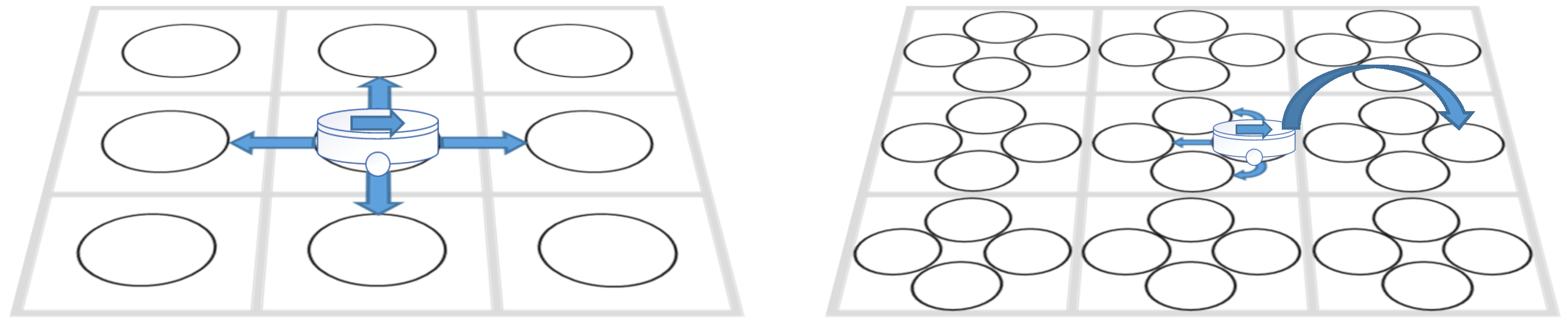
2.2. AGV-Referenced Action Space
2.3. Map Modeling
- Accurate representation of different map elements, such as obstacles, storage locations, and transportation paths;
- Explicit definition of connectivity between nodes, incorporating AGV motion constraints.
2.3.1. Classification of Obstacles in Manufacturing Environment
- Known, Movable: Other online AGVs, automated doors;
- Unknown, Movable: Workers, forklifts;
- Known, Fixed: Factory layout, pre-registered shelves;
- Unknown, Fixed: Unregistered equipment, offline AGVs.
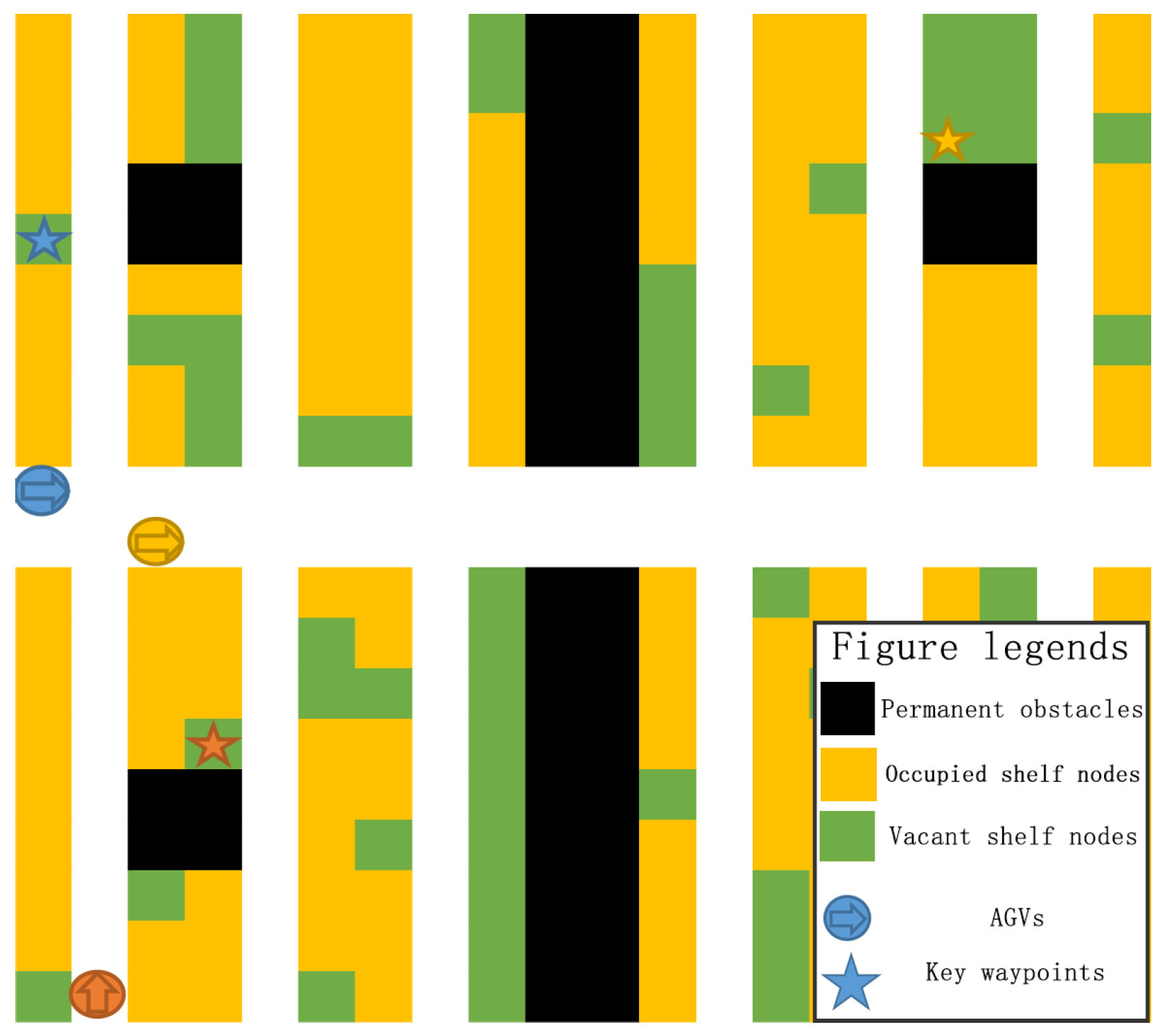
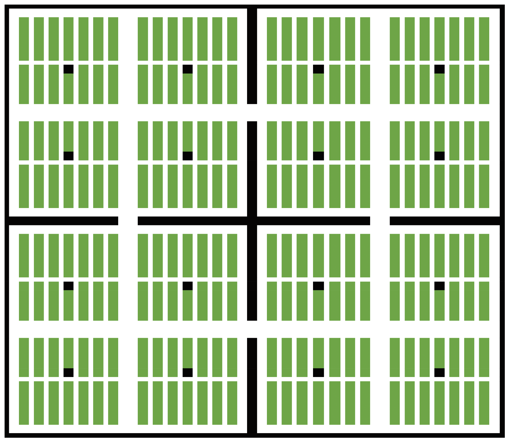
2.3.2. Grid-Based Map Representation
- Black cells represent permanent obstacles, such as factory walls and pillars. AGVs cannot enter these areas;
- Yellow cells represent occupied shelf nodes. Empty AGVs can pass through, but AGVs carrying a shelf cannot;
- Green cells represent vacant shelf nodes, where AGVs can move freely;
- White cells represent reserved passageway, ensuring accessibility to all shelf nodes;
- AGVs are depicted as colored icons, and their current destination is marked by a matching star icon.
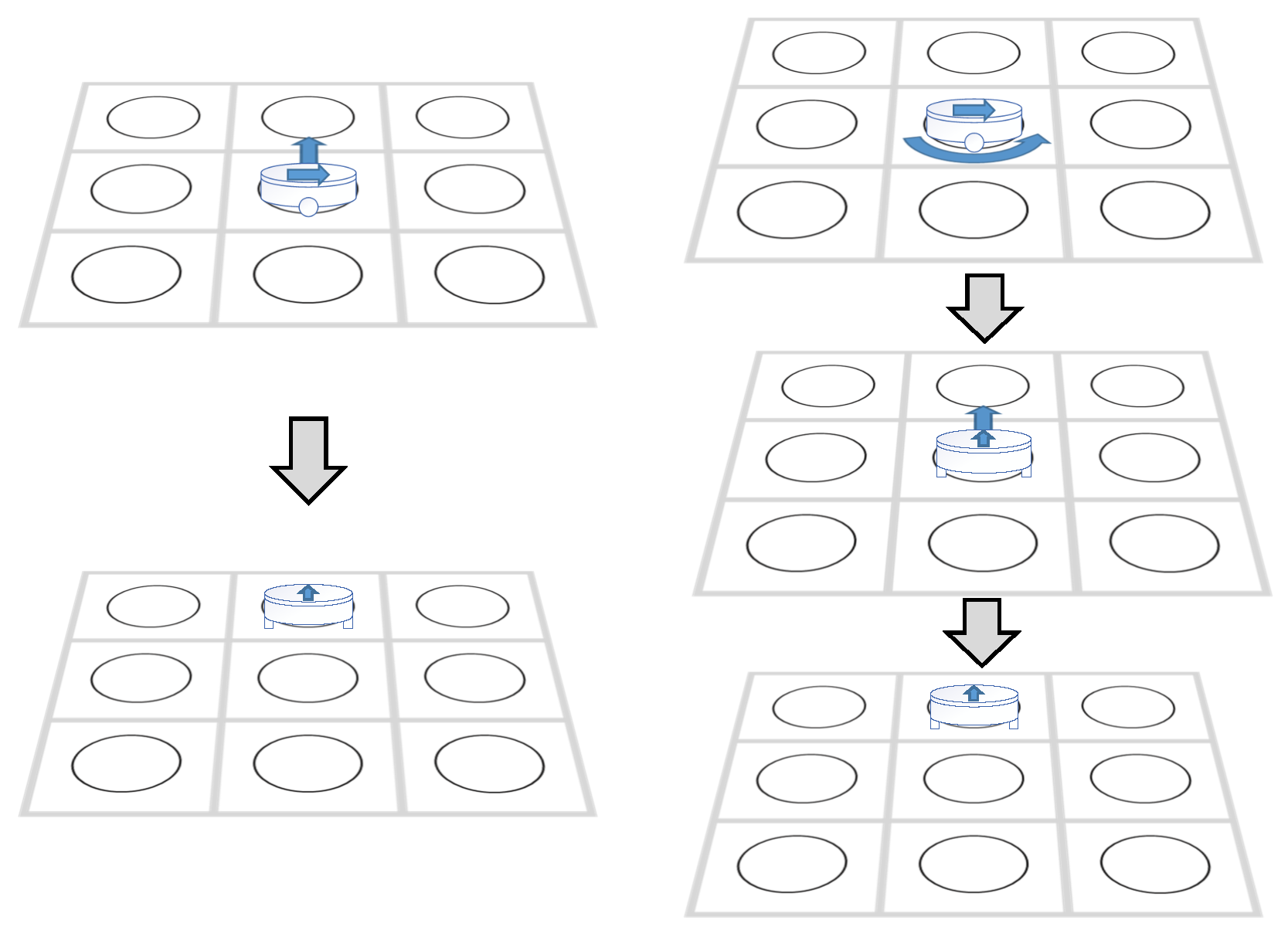
2.3.3. Directional Nodes
3. Macro-Control and Micro-Autonomy Pathfinding Strategy
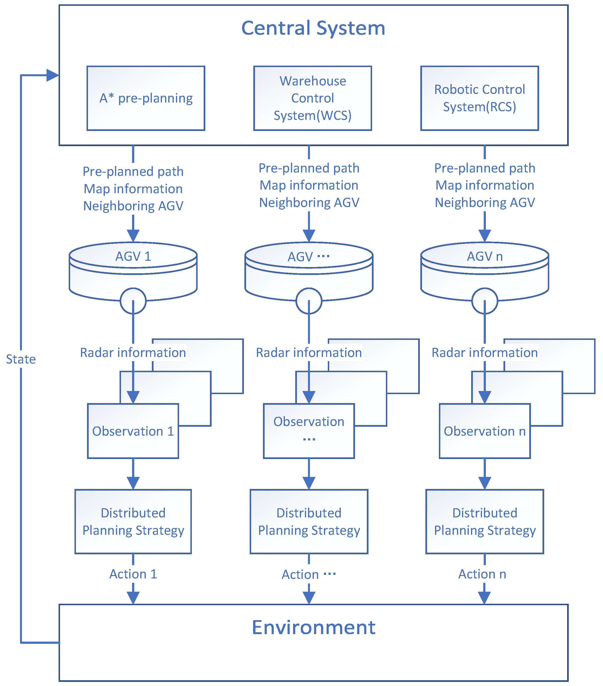
3.1. Overall Design of Macro-Control and Micro-Autonomy Pathfinding System
- Macro-Level (Centralized Pre-Planning): The central system pre-plans AGV paths using an modified A* algorithm, ignoring potential dynamic obstacles and AGV conflicts. This pre-planned path serves as a guideline for AGVs.
- Micro-Level (Distributed Decision Making): Each AGV autonomously decides its next move based on the pre-planned path from the central system, real-time local obstacle detection, and neighboring AGV states (shared via communication).
3.1.1. Execution Process
- Task Decomposition: The central system first breaks down transport tasks that are too difficult for a single AGV to complete, such as cross-floor or cross-workshop tasks, into smaller subtasks that a single AGV can handle. For each subtask, the system identifies key waypoints like a pickup node and a drop-off node. If the loading or unloading involves other machinery, a pre-transfer waiting point is also defined.
- Task Scheduling: Then, the central system assigns subtasks. Subtasks without prerequisites, or whose prerequisite tasks have been assigned, are then allocated to AGVs based on the priority of the task and the estimated distance from the A* pre-planned path. Under full-load operation with no idle AGVs available, each AGV, upon completion of its current subtask, immediately requests and receives the next subtask from the central system.
- Pathfinding: For each AGV that actively executes a subtask, the central system uses A* to calculate a pre-planned path from its current node to the next critical waypoint. The map, pre-planned path, and positions of the neighbor AGVs are transmitted to the vehicle. The AGV then combines this information with real-time LiDAR data and runs its distributed planning strategy to dynamically avoid obstacles and refine its local path.
- Feedback and Calibration: Upon entering each new node, the AGV scans the ground code (a QR code on the floor) to recalibrate its position and reports its updated coordinates to the central system. If the AGV has deviated from its original pre-planned route, the central system recalculates and issues an updated path.
3.1.2. System Robustness Discussion
3.2. Centralized Planning with Modified A*
3.2.1. A* Algorithm Overview
3.2.2. Enhancements for AGV Path Finding
- AGV-Referenced Action Space: The action space is updated to move forward, rotate 90° left, rotate 90° right, rotate 180° back, and then wait. A* now uses specific rotating actions to apply turning penalty corrections.
- Directional Spatial Nodes: Instead of treating locations as simple X-Y coordinates, each AGV state includes directional information (North, East, South, West) and represents it using directional spatial nodes. Accordingly, when adding nodes to the open list or close list, the algorithm also considers the directional attributes of the nodes.
- Modified Heuristic Function: A rotation penalty is introduced. It is based on the expected number of rotation actions and is combined with the Manhattan distance to form a revised heuristic function . This allows for a more accurate estimation of the value of each node and helps reduce unnecessary turns.
3.3. Distributed Planning Strategy
- Double Dueling Deep Q-Network (D3QN) [40]: Improves Q-value estimation stability and prevents overestimation errors;
- Prioritized Experience Replay (PER) [41]: Enhances training efficiency by prioritizing high-impact experience samples;
- -DAgger Imitation Learning: Combines reinforcement learning and imitation learning, using the parameter to control whether to use expert demonstrations (A* pre-planned path) for training. It improves learning efficiency while avoiding over-reliance on expert demonstrations, allowing the system to adapt to situations where the expert strategy has flaws.
3.3.1. PER-D3QN Reinforcement Learning
3.3.2. -DAgger Imitation Learning Strategy
- With probability : It executes the standard reinforcement learning process and uses -greedy policy to select an action; with probability , it selects a random action from the action space; with probability , it selects the best action according to the evaluation network. Consequently, the overall probability that the final model takes a random action is .
- With probability : It imitates the expert demonstrations (A* pre-planned path), uses A* to plan path, and chooses the action from the planned path. After receiving feedback from the environment, the expert demonstrations will be stored in the experience pool for learning.
3.3.3. Action and Observation Space Design
Action Space
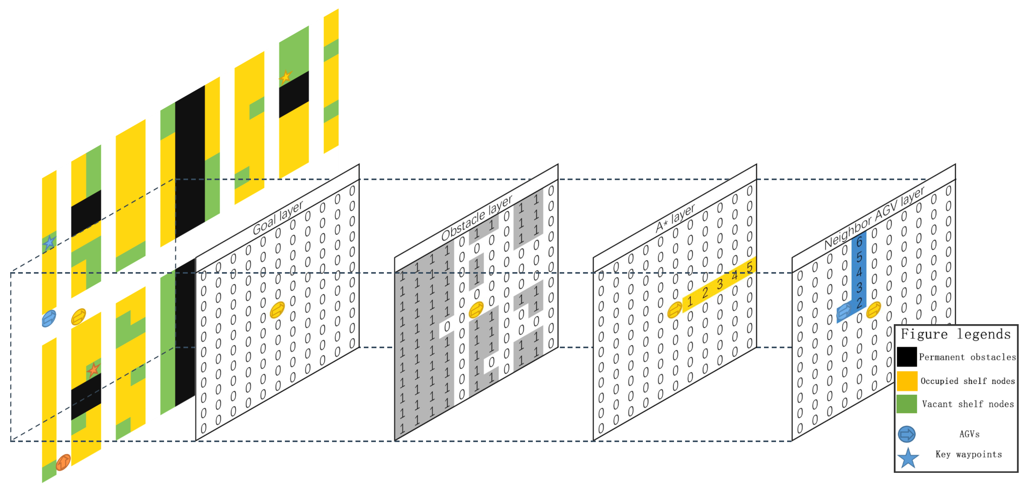
Observation Space
- Goal Layer: This layer represents the relative position of the key waypoint that the AGV must reach. Using the AGV’s own frame of reference, the matrix center corresponds to the AGV’s location. If the waypoint lies within the AGV’s nearby cells, the corresponding matrix entry is set to 1; otherwise, it remains at 0.
- Obstacles Layer: This layer depicts all potential obstacles around the AGV by fusing the global map provided by the central system with the AGV’s LiDAR data. Cells containing obstacles have a value of 1, and free cells are 0. In addition, the loaded AGVs treat shelves as obstacles, whereas the unloaded AGVs freely pass beneath shelves, which are then not considered obstacles.
- A* Pre-Planned Path Layer: This layer encodes the pre-planned path from the central system to guide the AGV. Starting from the center of matrix (the AGV position) and extending outward, each cell on the planned path is assigned the number of time steps required to reach it. If a single grid cell appears in multiple time steps (e.g., during a turn), the maximum value is used.
- Neighbor AGV Layer: This layer conveys the relative positions and expected trajectories of the surrounding AGVs. Similarly to the A* Pre-Planned Path Layer, each neighboring AGV’s A* pre-planned path radiates outward from its current position. Cells on these paths are set to the time steps needed to arrive there, taking the maximum value where the paths overlap or intersect.
3.3.4. Reward Design
4. Result and Discussion
4.1. Experimental Setup
4.1.1. Hardware and Software Environment
- System: Windows 11;
- CPU: Intel Core i5-13600KF (Intel, Santa Clara, CA, USA);
- GPU: NVIDIA GeForce RTX 3060 (NVIDIA, Santa Clara, CA, USA);
- RAM: 32 GB;
- Program Language: Python 3.8.20;
- Program Framework: PaddlePaddle.
4.1.2. Hyperparameters
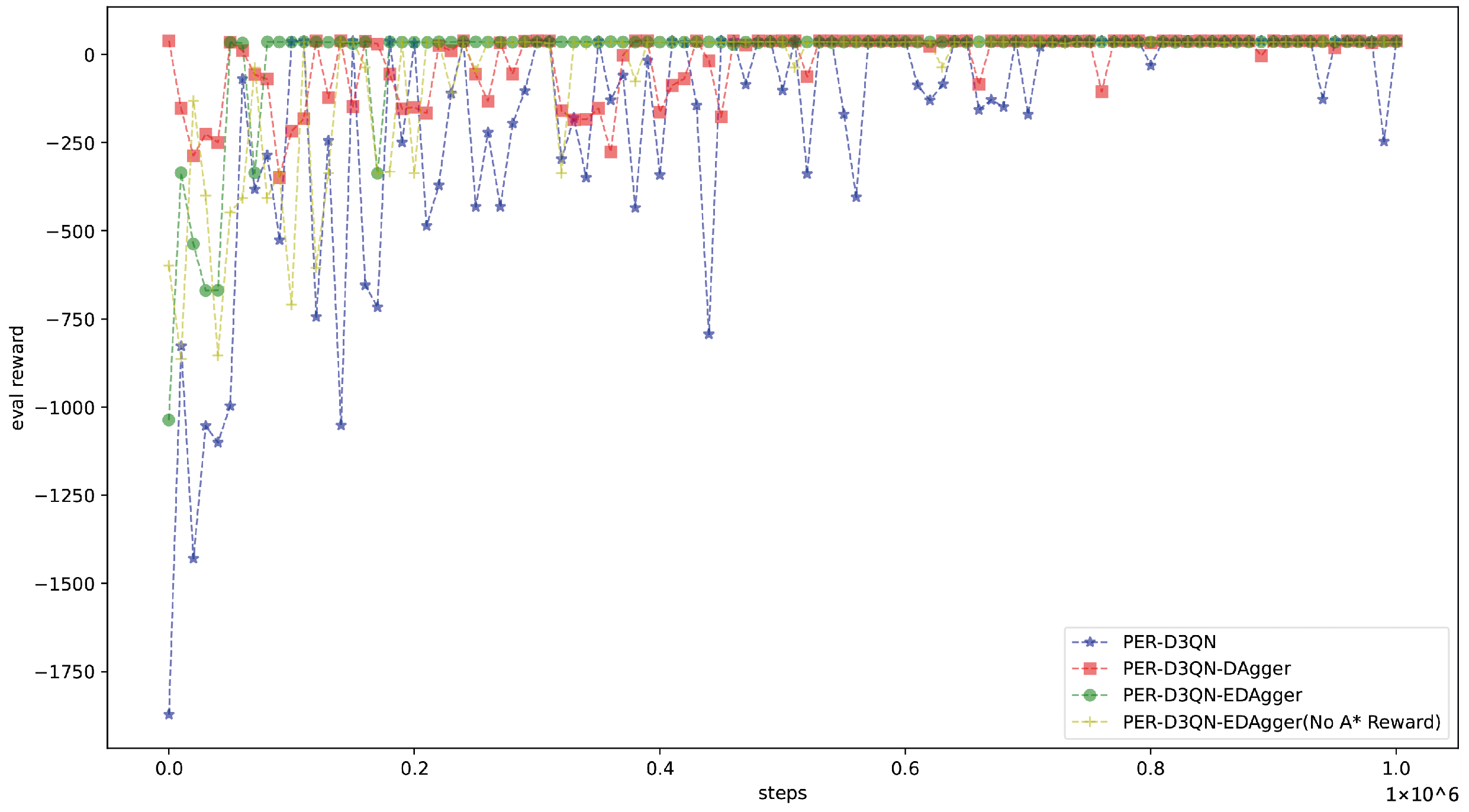
4.2. PER-D3QN-EDAgger Model Training
- Full PER-D3QN-EDAgger (complete model);
- PER-D3QN-EDAgger without A* rewards (removing the incentive for following the A* pre-planned path);
- PER-D3QN without IL (removing the DAgger-based expert demonstrations; reinforcement learning alone);
- PER-D3QN with pre-training using DAgger (expert demonstrations only used for initialization).
- Shelf Initialization: In the beginning, the shelf nodes generate shelves based on random numbers in to reconstruct obstacle layouts. If the random number is less than the shelf density coefficient , the cell is marked as occupied by a shelf; otherwise it remains free, allowing the AGVs to pass freely. During training, is sampled uniformly from 0.1 to 0.8. Only natural, the larger is, the higher the obstacle density of the environment.
- AGV Placement: The number of AGVs is chosen uniformly from 1 to 20. Except when , one AGV serves as a dynamic obstacle, making unpredictable random moves. In the environment configuration, all AGVs are initially placed at random in free-road cells.
- Task Generation: Each training episode randomly creates between 10 and 30 transport tasks, each with exactly two key waypoints. For each task, one occupied shelf cell and one free shelf cell are selected without replacement as the start and end points. If there are too few of either shelf cell, the environment well be reinitialized. Because free-road cells are reserved in advance, no task is ever rendered unreachable.
4.3. Dynamic Multi-Stage Path Planning Experiments
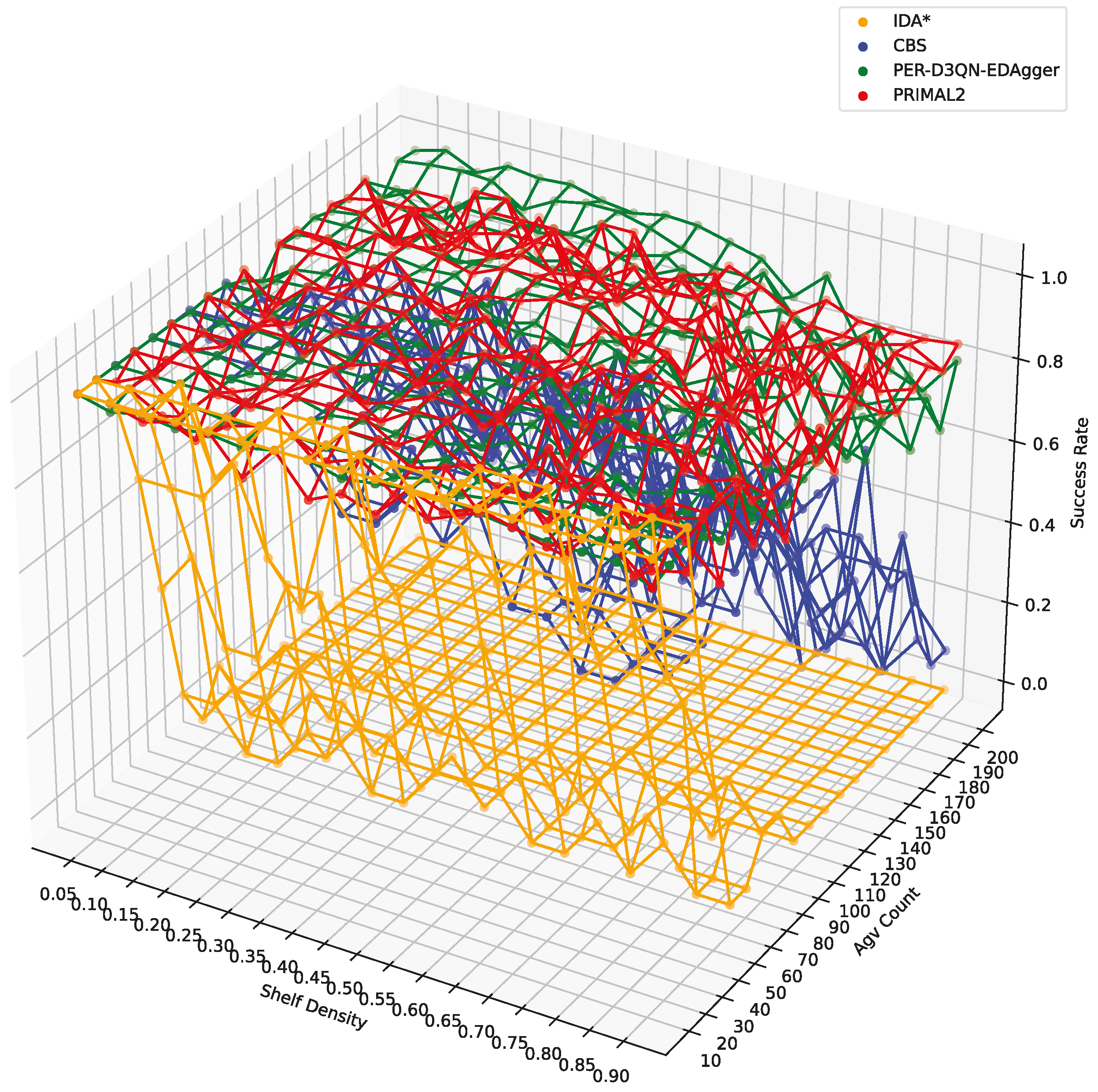
4.3.1. Task Completion Rate
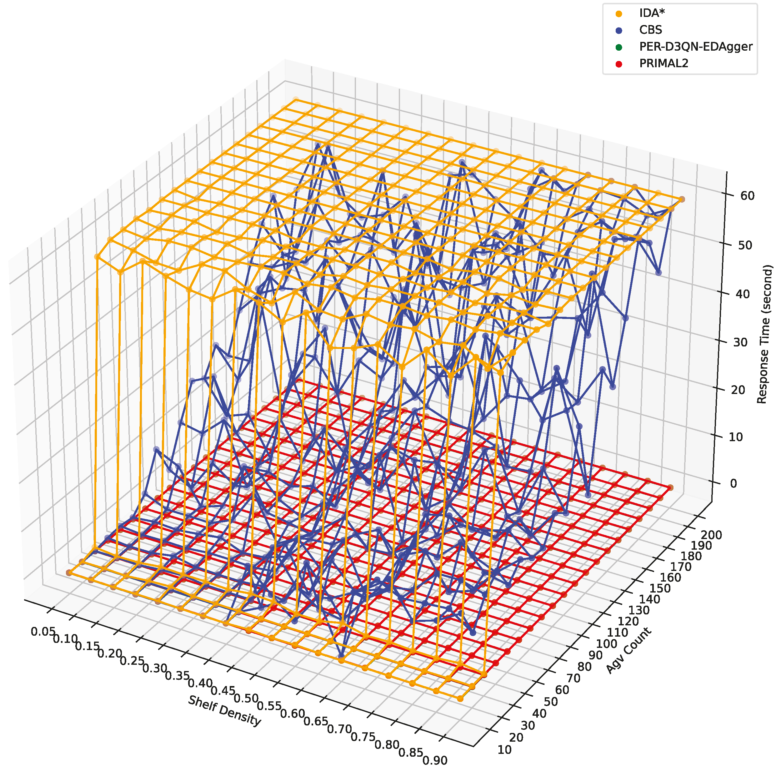
4.3.2. Response Time
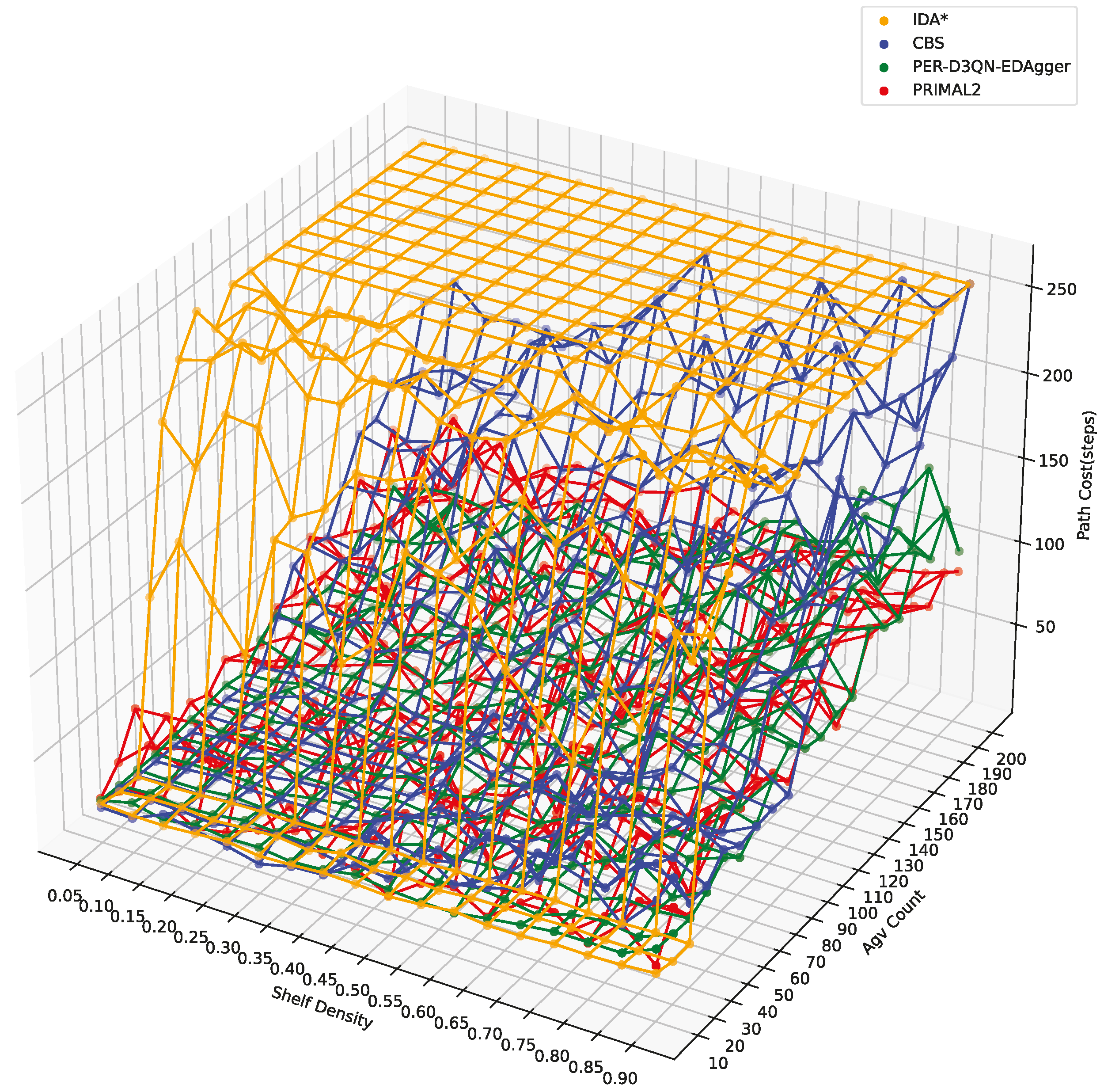
4.3.3. Average Path Cost
5. Conclusions
- Macro-Level (Centralized Planning): The central system decomposes multi-stage transportation tasks and pre-planned paths for each subtask using an modified A* algorithm.
- Micro-Level (Distributed Planning): Each AGV uses a deep reinforcement learning-based navigation strategy, trained with PER-D3QN-EDAgger, to make real-time decisions by considering local obstacles, pre-planned paths, and neighboring AGVs.
6. Future Prospects
Author Contributions
Funding
Institutional Review Board Statement
Informed Consent Statement
Data Availability Statement
Conflicts of Interest
References
- Ge, X.; Li, L.; Chen, H. Research on online scheduling method for flexible assembly workshop of multi-agv system based on assembly island mode. In Proceedings of the 2021 IEEE 7th International Conference on Cloud Computing and Intelligent Systems (CCIS), Xi’an, China, 7–8 November 2021; IEEE: Piscataway, NJ, USA, 2021; pp. 371–375. [Google Scholar]
- De Ryck, M.; Versteyhe, M.; Debrouwere, F. Automated guided vehicle systems, state-of-the-art control algorithms and techniques. J. Manuf. Syst. 2020, 54, 152–173. [Google Scholar] [CrossRef]
- Bhardwaj, A.; Sam, L.; Bhardwaj, A.; Martín-Torres, F.J. LiDAR remote sensing of the cryosphere: Present applications and future prospects. Remote Sens. Environ. 2016, 177, 125–143. [Google Scholar] [CrossRef]
- Wild, G.; Hinckley, S. Acousto-ultrasonic optical fiber sensors: Overview and state-of-the-art. IEEE Sens. J. 2008, 8, 1184–1193. [Google Scholar] [CrossRef]
- Stern, R. Multi-agent path finding—An overview. In Artificial Intelligence: 5th RAAI Summer School, Dolgoprudny, Russia, 4–7 July 2019, Tutorial Lectures; Springer: Cham, Switzerland, 2019; pp. 96–115. [Google Scholar]
- Standley, T. Finding optimal solutions to cooperative pathfinding problems. Proc. AAAI Conf. Artif. Intell. 2010, 24, 173–178. [Google Scholar] [CrossRef]
- Wagner, G.; Choset, H. Subdimensional expansion for multirobot path planning. Artif. Intell. 2015, 219, 1–24. [Google Scholar] [CrossRef]
- Guo, T.; Sun, Y.; Liu, Y.; Liu, L.; Lu, J. An automated guided vehicle path planning algorithm based on improved a* and dynamic window approach fusion. Appl. Sci. 2023, 13, 10326. [Google Scholar] [CrossRef]
- Chen, D.; Liu, X.; Liu, S. Improved A-star algorithm based on the two-way search for path planning of automated guided vehicle. J. Comput. Appl. 2021, 41, 309–313. [Google Scholar]
- Sharon, G.; Stern, R.; Felner, A.; Sturtevant, N.R. Conflict-based search for optimal multi-agent pathfinding. Artif. Intell. 2015, 219, 40–66. [Google Scholar] [CrossRef]
- Boyarski, E.; Felner, A.; Harabor, D.; Stuckey, P.J.; Cohen, L.; Li, J.; Koenig, S. Iterative-deepening conflict-based search. In Proceedings of the International Joint Conference on Artificial Intelligence-Pacific Rim International Conference on Artificial Intelligence 2020, Virtual Event, 11–17 July 2020; Association for the Advancement of Artificial Intelligence (AAAI): Washington, DC, UDA, 2020; pp. 4084–4090. [Google Scholar]
- Boyarski, E.; Felner, A.; Le Bodic, P.; Harabor, D.D.; Stuckey, P.J.; Koenig, S. F-aware conflict prioritization & improved heuristics for conflict-based search. Proc. AAAI Conf. Artif. Intell. 2021, 35, 12241–12248. [Google Scholar]
- Chan, S.H.; Li, J.; Gange, G.; Harabor, D.; Stuckey, P.J.; Koenig, S. ECBS with flex distribution for bounded-suboptimal multi-agent path finding. In Proceedings of the Fourteenth International Symposium on Combinatorial Search, Guangzhou, China, 26–30 July 2021; Volume 12, pp. 159–161. [Google Scholar]
- Rahman, M.; Alam, M.A.; Islam, M.M.; Rahman, I.; Khan, M.M.; Iqbal, T. An adaptive agent-specific sub-optimal bounding approach for multi-agent path finding. IEEE Access 2022, 10, 22226–22237. [Google Scholar] [CrossRef]
- Yu, J.; Li, R.; Feng, Z.; Zhao, A.; Yu, Z.; Ye, Z.; Wang, J. A novel parallel ant colony optimization algorithm for warehouse path planning. J. Control Sci. Eng. 2020, 2020, 5287189. [Google Scholar] [CrossRef]
- Xu, L.; Liu, Y.; Wang, Q. Application of adaptive genetic algorithm in robot path planning. Comput. Eng. Appl. 2020, 56, 36–41. [Google Scholar]
- Chen, J.; Liang, J.; Tong, Y. Path planning of mobile robot based on improved differential evolution algorithm. In Proceedings of the 2020 16th International Conference on Control, Automation, Robotics and Vision (ICARCV), Shenzhen, China, 13–15 December 2020; IEEE: Piscataway, NJ, USA, 2020; pp. 811–816. [Google Scholar]
- Niu, Q.; Li, M.; Zhao, Y. Research on improved artificial potential field method for AGV path planning. Mach. Tool Hydraul. 2022, 50, 19–24. [Google Scholar]
- Qiuyun, T.; Hongyan, S.; Hengwei, G.; Ping, W. Improved particle swarm optimization algorithm for AGV path planning. IEEE Access 2021, 9, 33522–33531. [Google Scholar] [CrossRef]
- Abed-Alguni, B.H.; Paul, D.J.; Chalup, S.K.; Henskens, F.A. A comparison study of cooperative Q-learning algorithms for independent learners. Int. J. Artif. Intell. 2016, 14, 71–93. [Google Scholar]
- De Witt, C.S.; Gupta, T.; Makoviichuk, D.; Makoviychuk, V.; Torr, P.H.; Sun, M.; Whiteson, S. Is independent learning all you need in the starcraft multi-agent challenge? arXiv 2020, arXiv:2011.09533. [Google Scholar]
- Sunehag, P.; Lever, G.; Gruslys, A.; Czarnecki, W.M.; Zambaldi, V.; Jaderberg, M.; Lanctot, M.; Sonnerat, N.; Leibo, J.Z.; Tuyls, K.; et al. Value-decomposition networks for cooperative multi-agent learning. arXiv 2017, arXiv:1706.05296. [Google Scholar]
- Rashid, T.; Samvelyan, M.; De Witt, C.S.; Farquhar, G.; Foerster, J.; Whiteson, S. Monotonic value function factorisation for deep multi-agent reinforcement learning. J. Mach. Learn. Res. 2020, 21, 7234–7284. [Google Scholar]
- Son, K.; Kim, D.; Kang, W.J.; Hostallero, D.E.; Yi, Y. Qtran: Learning to factorize with transformation for cooperative multi-agent reinforcement learning. In Proceedings of the 36th International Conference on Machine Learning, Long Beach, CA, USA, 9–15 June 2019; pp. 5887–5896. [Google Scholar]
- Lowe, R.; Wu, Y.I.; Tamar, A.; Harb, J.; Pieter Abbeel, O.; Mordatch, I. Multi-agent actor-critic for mixed cooperative-competitive environments. In Advances in Neural Information Processing Systems; MIT Press: Cambridge, MA, USA, 2017; Volume 30. [Google Scholar]
- Foerster, J.; Farquhar, G.; Afouras, T.; Nardelli, N.; Whiteson, S. Counterfactual multi-agent policy gradients. Proc. AAAI Conf. Artif. Intell. 2018, 32, 2974–2982. [Google Scholar] [CrossRef]
- Rabinowitz, N.; Perbet, F.; Song, F.; Zhang, C.; Eslami, S.A.; Botvinick, M. Machine theory of mind. In Proceedings of the 35th International Conference on Machine Learning, Stockholm, Sweden, 10–15 July 2018; pp. 4218–4227. [Google Scholar]
- Sartoretti, G.; Kerr, J.; Shi, Y.; Wagner, G.; Kumar, T.S.; Koenig, S.; Choset, H. Primal: Pathfinding via reinforcement and imitation multi-agent learning. IEEE Robot. Autom. Lett. 2019, 4, 2378–2385. [Google Scholar] [CrossRef]
- Damani, M.; Luo, Z.; Wenzel, E.; Sartoretti, G. PRIMAL_2: Pathfinding via reinforcement and imitation multi-agent learning-lifelong. IEEE Robot. Autom. Lett. 2021, 6, 2666–2673. [Google Scholar] [CrossRef]
- Liu, Z.; Chen, B.; Zhou, H.; Koushik, G.; Hebert, M.; Zhao, D. Mapper: Multi-agent path planning with evolutionary reinforcement learning in mixed dynamic environments. In Proceedings of the 2020 IEEE/RSJ International Conference on Intelligent Robots and Systems (IROS), Las Vegas, NV, USA, 24 October 2020–24 January 2021; IEEE: Piscataway, NJ, USA, 2021; pp. 11748–11754. [Google Scholar]
- Guan, H.; Gao, Y.; Zhao, M.; Yang, Y.; Deng, F.; Lam, T.L. Ab-mapper: Attention and bicnet based multi-agent path planning for dynamic environment. In Proceedings of the 2022 IEEE/RSJ International Conference on Intelligent Robots and Systems (IROS), Kyoto, Japan, 23–27 October 2022; IEEE: Piscataway, NJ, USA, 2022; pp. 13799–13806. [Google Scholar]
- Li, W.; Chen, H.; Jin, B.; Tan, W.; Zha, H.; Wang, X. Multi-agent path finding with prioritized communication learning. In Proceedings of the 2022 International Conference on Robotics and Automation (ICRA), Philadelphia, PA, USA, 23–27 May 2022; IEEE: Piscataway, NJ, USA, 2022; pp. 10695–10701. [Google Scholar]
- Li, Q.; Lin, W.; Liu, Z.; Prorok, A. Message-aware graph attention networks for large-scale multi-robot path planning. IEEE Robot. Autom. Lett. 2021, 6, 5533–5540. [Google Scholar] [CrossRef]
- Ma, Z.; Luo, Y.; Pan, J. Learning selective communication for multi-agent path finding. IEEE Robot. Autom. Lett. 2021, 7, 1455–1462. [Google Scholar] [CrossRef]
- Skrynnik, A.; Yakovleva, A.; Davydov, V.; Yakovlev, K.; Panov, A.I. Hybrid policy learning for multi-agent pathfinding. IEEE Access 2021, 9, 126034–126047. [Google Scholar] [CrossRef]
- Ni, P.; Mao, P.; Wang, N.; Yang, M. Robot path planning based on improved A-DDQN algorithm. J. Syst. Simul. 2024. [Google Scholar] [CrossRef]
- Wang, B.; Liu, Z.; Li, Q.; Prorok, A. Mobile robot path planning in dynamic environments through globally guided reinforcement learning. IEEE Robot. Autom. Lett. 2020, 5, 6932–6939. [Google Scholar] [CrossRef]
- Bai, Z.; Pang, H.; He, Z.; Zhao, B.; Wang, T. Path planning of autonomous mobile robot in comprehensive unknown environment using deep reinforcement learning. IEEE Internet Things J. 2024, 11, 22153–22166. [Google Scholar] [CrossRef]
- Ferguson, D.; Likhachev, M.; Stentz, A. A guide to heuristic-based path planning. In Proceedings of the International Workshop on Planning Under Uncertainty for Autonomous Systems, International Conference on Automated Planning and Scheduling (ICAPS), Monterey, CA, USA, 5–10 June 2005; pp. 9–18. [Google Scholar]
- Hessel, M.; Modayil, J.; Van Hasselt, H.; Schaul, T.; Ostrovski, G.; Dabney, W.; Horgan, D.; Piot, B.; Azar, M.; Silver, D. Rainbow: Combining improvements in deep reinforcement learning. Proc. AAAI Conf. Artif. Intell. 2018, 32, 3215–3222. [Google Scholar] [CrossRef]
- Schaul, T.; Quan, J.; Antonoglou, I.; Silver, D. Prioritized experience replay. arXiv 2015, arXiv:1511.05952. [Google Scholar]
- Mnih, V.; Kavukcuoglu, K.; Silver, D.; Rusu, A.A.; Veness, J.; Bellemare, M.G.; Graves, A.; Riedmiller, M.; Fidjeland, A.K.; Ostrovski, G.; et al. Human-level control through deep reinforcement learning. Nature 2015, 518, 529–533. [Google Scholar] [CrossRef]
- Van Hasselt, H.; Guez, A.; Silver, D. Deep reinforcement learning with double q-learning. Proc. AAAI Conf. Artif. Intell. 2016, 30, 2094–2100. [Google Scholar] [CrossRef]
- Wang, Z.; Schaul, T.; Hessel, M.; Hasselt, H.; Lanctot, M.; Freitas, N. Dueling network architectures for deep reinforcement learning. In Proceedings of the 33rd International Conference on Machine Learning, New York, NY, USA, 19–24 June 2016; pp. 1995–2003. [Google Scholar]
- Ross, S.; Gordon, G.; Bagnell, D. A reduction of imitation learning and structured prediction to no-regret online learning. In Proceedings of the Fourteenth International Conference on Artificial Intelligence and Statistics, Fort Lauderdale, FL, USA, 11–13 April 2011; pp. 627–635. [Google Scholar]

| Category | Definition | Examples |
|---|---|---|
| Fixed or Movable | Fixed obstacles cannot move and only affect the connectivity of the grid they occupy; movable obstacles can move and may affect the connectivity of multiple grid cells within a single timestep. | Fixed: Factory walls, pre-registered shelves. Movable: Workers, forklifts, other AGVs. |
| Known or Unknown | Known obstacles are registered in the central system, with their state globally shared; Unknown obstacles are not registered in the central system; only nearby AGVs can detect it using their own sensing devices. | Known: Pre-mapped factory layout, online AGVs. Unknown: Unregistered or offline equipment, workers. |
| Situation | The Angle Between AGV’s Direction and Its Target | (Penalty) |
|---|---|---|
| The AGV’s target is directly in front of AGV. | angle = 0° | 0 |
| The AGV’s target is directly behind AGV. | angle = 180° | 1 |
| The AGV’s target is directly on the left or right side of AGV. | angle = 90° | 1 |
| The AGV’s target is on the front-left or front-right of AGV. | 0° < angle < 90° | 1 |
| The AGV’s target is on the rear-left or rear-right of AGV. | 90° < angle < 180° | 2 |
| Condition | Reward |
|---|---|
| AGV reaches goal | 10 |
| AGV takes any action | −0.1 |
| AGV follows the A* path to take action | 0.1 |
| Collision or invalid move | −2 |
| Parameter | Value |
|---|---|
| Discount Factor | 0.99 |
| Greedy Factor | 0.9 to 0.1 (over 50,000 steps) |
| Prioritization Factor | 1 |
| Factor | 0.1 |
| Learning Rate | 0.0003 to 0.00001 (over 50,000 steps) |
| Batch Size | 128 |
| Experience Replay Buffer Size | 100,000 |
| Target Network Update Frequency | Every 2500 steps |
| Train Total Steps | 1,000,000 |
| Warmup Size | 10,000 |
| AGV Count | 1–10 | 1–10 | 11–20 | 11–20 | |
|---|---|---|---|---|---|
| Shelf Density | 0.05–0.45 | 0.50–0.90 | 0.05–0.45 | 0.50–0.90 | |
| Average | ID A* | 0.420 | 0.422 | 0 | 0 |
| CBS | 0.982 | 0.854 | 0.638 | 0.488 | |
| Success Rate | PER-D3QN-EDAgger | 0.994 | 0.956 | 0.984 | 0.888 |
| PRIMAL2 | 0.975 | 0.943 | 0.939 | 0.891 | |
| Average | ID A* | 41.634 | 41.386 | 60 | 60 |
| CBS | 3.415 | 13.691 | 29.632 | 41.987 | |
| Response Time(s) | PER-D3QN-EDAgger | 0.012 | 0.010 | 0.012 | 0.013 |
| PRIMAL2 | 0.026 | 0.024 | 0.025 | 0.026 | |
| Average Path | ID A* | 164.758 | 165.506 | 256 | 256 |
| CBS | 20.517 | 49.265 | 106.266 | 149.899 | |
| Cost (steps) | PER-D3QN-EDAgger | 26.094 | 40.038 | 45.247 | 79.576 |
| PRIMAL2 | 39.698 | 43.524 | 60.636 | 73.311 |
Disclaimer/Publisher’s Note: The statements, opinions and data contained in all publications are solely those of the individual author(s) and contributor(s) and not of MDPI and/or the editor(s). MDPI and/or the editor(s) disclaim responsibility for any injury to people or property resulting from any ideas, methods, instructions or products referred to in the content. |
© 2025 by the authors. Licensee MDPI, Basel, Switzerland. This article is an open access article distributed under the terms and conditions of the Creative Commons Attribution (CC BY) license (https://creativecommons.org/licenses/by/4.0/).
Share and Cite
Le, J.; He, L.; Zheng, J. A Macro-Control and Micro-Autonomy Pathfinding Strategy for Multi-Automated Guided Vehicles in Complex Manufacturing Scenarios. Appl. Sci. 2025, 15, 5249. https://doi.org/10.3390/app15105249
Le J, He L, Zheng J. A Macro-Control and Micro-Autonomy Pathfinding Strategy for Multi-Automated Guided Vehicles in Complex Manufacturing Scenarios. Applied Sciences. 2025; 15(10):5249. https://doi.org/10.3390/app15105249
Chicago/Turabian StyleLe, Jiahui, Lili He, and Junhong Zheng. 2025. "A Macro-Control and Micro-Autonomy Pathfinding Strategy for Multi-Automated Guided Vehicles in Complex Manufacturing Scenarios" Applied Sciences 15, no. 10: 5249. https://doi.org/10.3390/app15105249
APA StyleLe, J., He, L., & Zheng, J. (2025). A Macro-Control and Micro-Autonomy Pathfinding Strategy for Multi-Automated Guided Vehicles in Complex Manufacturing Scenarios. Applied Sciences, 15(10), 5249. https://doi.org/10.3390/app15105249