Abstract
Accurately predicting the permeability of coarse-grained soils is crucial for ensuring geotechnical safety and performance. In this study, 64 coarse-grained soil (CGS) samples were designed using a negative exponential gradation equation (NEGE), and computational fluid dynamics–discrete element method (CFD-DEM) coupled seepage simulations were conducted to generate a permeability coefficient (k) dataset comprising 256 entries under varying porosity and gradation conditions. Three machine learning models—a neural network model (BPNN), a regression model (GPR), and a tree-based model (RF)—were employed to predict k, with hyperparameters optimized via particle swarm optimization (PSO) and four-fold cross-validation applied to improve generalization. Gray relational analysis (GRA) revealed that all input parameters (α, β, dmax, n) significantly influence k (R > 0.6). The interquartile range (IQR) method confirmed data suitability for modeling. Among the models, BPNN achieved the best performance (R2 = 0.99, MAE = 1.5, RMSE = 2.9, U95 = 0.4), effectively capturing the complex nonlinear relationship between gradation and permeability. GPR (R2 = 0.92) was hindered by kernel selection and noise sensitivity, while RF (R2 = 0.97) was limited by its discrete regression nature. Compared to a traditional empirical model (R2 = 0.9031), BPNN improved prediction accuracy by 10.13%, demonstrating the advantage of data-driven methods for evaluating CGS permeability.
1. Introduction
Coarse-grained soils (CGSs) are defined as soils in which particles with diameters ranging from 0.075 to 60 mm constitute more than 50% of the total mass [1,2,3]. They are widely used in the construction of geotechnical structures such as dams and embankments, as well as various permeable structures and facilities, due to their favorable engineering properties, including high compaction performance, large permeability coefficient, and high shear strength. Permeability is a fundamental soil property that plays a critical role in determining the stability and functionality of geotechnical structures. It is commonly characterized by the permeability coefficient, the accurate determination of which has been a longstanding focus and challenge in both academic and engineering communities [4,5,6]. The permeability coefficient of soils is typically obtained through experimental testing [7,8,9].
The permeability coefficient of CGS is typically determined through experimental testing [10,11,12]. However, permeability tests for CGSs present challenges such as large specimen size, difficulties in specimen preparation, and long testing durations. Consequently, extensive efforts have been made to develop predictive formulas for the permeability coefficient. Existing studies indicate that key factors influencing the permeability of CGSs include particle size distribution [13,14], particle shape [15,16,17], pore characteristics [18,19], mineral composition [20,21], temperature [22,23], and fluid properties [24]. For a given type of CGS (i.e., soils with similar genesis and mineral composition, which are generally considered to be of the same type), the particle shape tends to be relatively consistent. Under such conditions, particle size distribution and pore characteristics become the two most critical factors governing permeability [25], as they largely determine the permeability coefficient. Therefore, in principle, the permeability coefficient of any given CGS should be computable based on parameters describing its particle size distribution and pore characteristics. Based on these parameters, numerous empirical models for predicting the permeability coefficient of CGSs have been developed by researchers worldwide. Notable examples include the Terzaghi model [26], Shahabi model [27], the modified Hazen model [28], as well as the Chapuis model [29]. Empirical models exhibit distinct advantages in predicting the permeability coefficient of coarse-grained soils, primarily due to their engineering applicability and rapid assessment capabilities. Empirical models, exemplified by the Kozeny–Carman equation, establish explicit mathematical relationships between permeability and particle size characteristics (e.g., effective particle size D10) as well as void ratio (e). These models require only a limited set of readily obtainable soil parameters, making them particularly suitable for on-site engineering decision-making. By leveraging statistical correlations derived from extensive laboratory test data, such models serve as efficient tools for the preliminary selection of coarse-grained fill materials and the early assessment of seepage risks, especially when applied to soils with relatively uniform gradation (e.g., well-graded sandy soils) and simple pore structures. However, the limitations of empirical models become particularly pronounced under complex conditions. The oversimplified physical assumptions hinder the accurate representation of multiscale pore connectivity in continuously graded coarse-grained soils. For instance, these models often neglect the nonlinear influence of particle angularity on tortuosity, leading to permeability coefficient prediction errors exceeding 50%. Second, model parameter sensitivity is highly dependent on boundary conditions. When soil gradation deviates significantly from standard ranges (e.g., uniformity coefficient Cu > 20) or when fine particles are interspersed, traditional empirical models may yield prediction errors spanning two to three orders of magnitude. More critically, these empirical formulas are fundamentally extrapolative fits to specific datasets. They neither elucidate the intrinsic physical mechanisms governing permeability evolution nor exhibit generalizability to novel engineering materials, such as recycled aggregate-stabilized soils, thereby limiting their broader applicability.
Given the mechanistic limitations and generalization bottlenecks of empirical models in predicting the permeability of complex CGSs, machine learning offers a novel paradigm for addressing the challenges of multifactor coupling. By autonomously extracting high-dimensional nonlinear interactions between gradation curve morphology and pore characteristics, data-driven models not only overcome the parameter sensitivity thresholds of traditional formulas but also leverage implicit feature mapping to capture key physical mechanisms, such as preferential seepage pathways. Compared to empirical equations that rely on manually imposed assumptions, machine learning optimizes feature weights adaptively and employs nonlinear function approximation, enabling cross-scale predictions from discrete particle size distributions to macroscopic permeability behavior even under limited specimen conditions. Furthermore, its superior prediction robustness significantly enhances the accuracy of permeability coefficient inversion for highly heterogeneous CGSs, establishing a technically rigorous yet practically viable approach for engineering applications.
In the field of permeability coefficient prediction for CGSs, various machine learning approaches have been systematically explored and validated for their effectiveness. The random forest algorithm was first employed to integrate the fractal dimension of the particle size distribution curve and pore tortuosity parameters, enabling a nonlinear mapping of the permeability coefficient for widely graded gravelly sands, with prediction accuracy improved by 62% compared to the traditional Hazen model [30]. A Bayesian-optimized support vector regression model has demonstrated its capability to stably capture the implicit relationships between particle shape parameters and permeability, even under small-specimen conditions, exhibiting significant advantages in extreme gradation scenarios where the uniformity coefficient (Cu > 15) is high [31]. To address high-dimensional feature coupling, a deep neural network architecture was designed with a dual-channel structure incorporating a gradation encoder and a physics-informed loss function, successfully decoupling the influence of particle contact force chain evolution on seepage pathways [32]). Additionally, the XGBoost algorithm has been embedded into a transfer learning framework, enabling knowledge migration across large-scale engineering databases and overcoming the limitations imposed by data scarcity in individual projects [33]. The attention-based long short-term memory (LSTM) network has been innovatively applied to capture the dynamic response of permeability coefficients over time, reducing prediction errors to 8.3% in coarse-grained subgrade soils under cyclic loading conditions [34]. Recent studies further confirm that graph convolutional networks (GCNs), incorporating discrete element simulation data, can effectively characterize the topological features of particle spatial arrangements, enhancing the accuracy of quantifying the contribution of three-dimensional pore structures to permeability to 92% [35,36,37,38].
In this investigation, 64 sets of CGS specimens were designed based on a negatively exponential continuous gradation equation, and computational fluid dynamics–discrete element method (CFD-DEM) simulations were conducted to model permeability tests, determining the permeability coefficients for each specimen under different porosity and gradation conditions. A comprehensive permeability coefficient database comprising 256 datasets would be constructed after correlation analysis and data preprocessing. Three machine learning approaches—neural network models, regression models, and tree-based models—would be employed to predict permeability coefficients, with a particle swarm optimization (PSO) algorithm introduced for global hyperparameter optimization. Four-fold cross-validation would be implemented to enhance data utilization and mitigate the impact of random data partitioning on model evaluation. Model performance would be assessed using multiple evaluation metrics, including the coefficient of determination (R2), root mean square error (RMSE), mean absolute error (MAE), and 95% uncertainty interval width (U95), and sensitivity analysis would be conducted to quantify the contribution of each input variable to the prediction outcomes. Finally, the superiority of machine learning methods in predicting the permeability behavior of CGSs would be validated through multidimensional comparisons with traditional empirical models and laboratory test results.
2. Influencing Factors of Permeability Coefficient
2.1. Porosity
Porosity is one of the key parameters governing the permeability coefficient of coarse-grained soils, exhibiting a distinctly nonlinear influence. The classical Kozeny–Carman equation establishes a positive correlation between permeability (k) and porosity (n), expressed as Equation (1). Experimental studies indicate that the permeability coefficient of uniform coarse sand can increase by two to three orders of magnitude when porosity rises from 0.25 to 0.35.
However, significant deviations from this theoretical relationship often occur in practical engineering applications due to spatial heterogeneity in pore structures, such as localized pore clustering and the formation of preferential flow channels. Fractal theory studies reveal that the permeability coefficient can increase by 40–60% when the fractal dimension (Df) rises by 0.1, reflecting enhanced pore connectivity at the same porosity. This effect becomes particularly pronounced under high compaction conditions (n < 0.2), where intensified grain-to-grain contact sharply increases pore tortuosity, reducing the sensitivity of permeability to porosity changes by over 80%. Under such conditions, the evolution of the contact network topology induced by gradation reconstruction becomes the dominant factor controlling permeability.
2.2. Gradation Behaviors
The permeability coefficient of continuously graded coarse-grained soils is closely linked to the shape of their gradation curve, primarily through the spatial arrangement of the particle skeleton, which regulates the connectivity of seepage pathways. The interplay between the uniformity coefficient (Cu, i.e., d60/d10) and the curvature coefficient [Cc, i.e., d302/(d60·d10)] governs the nesting efficiency of multiscale particles. When the gradation curve exhibits a “smoothly continuous” distribution (5 ≤ Cu ≤ 15 and Cc ≈ 1), particles of different sizes form a stable, progressively packed structure, significantly enhancing the continuity and flux of seepage paths. In contrast, a “steeply continuous” gradation (Cu > 20 or Cc deviating from 1) leads to excessive fine particles filling the voids between coarse grains, resulting in local pore blockage or rupture of flow channels, causing an exponential decay in permeability. Experimental studies indicate that when the fine particle content (<2 mm) in continuously graded soils exceeds 30%, the distribution pattern of interparticle contact force chains undergoes reconstruction. The originally interconnected preferential seepage pathways become fragmented into discrete networks by fine particle clusters. This topological heterogeneity at the microscale amplifies the sensitivity of macroscopic permeability behavior to gradation variations by approximately threefold, revealing a nonlinear coupling mechanism between gradation continuity and seepage efficiency. The continuous gradation of coarse-grained soils is characterized using the negative exponential gradation equation (NEGE) proposed by [39] (see Equation (2)). The proposed NEGE model enables accurate characterization of a wide range of continuous gradations—including concave, convex, linear, and S-shaped types—using only two parameters, which effectively reflect both the composition and distribution of soil particles.
where P is the percentage of soil mass smaller than a given particle size; d is the particle size; dmax is the maximum particle size; and α and β are fitting parameters controlling the shape of the curve and the degree of inclination, respectively.
3. Dataset Establishment
3.1. Data Acquisition
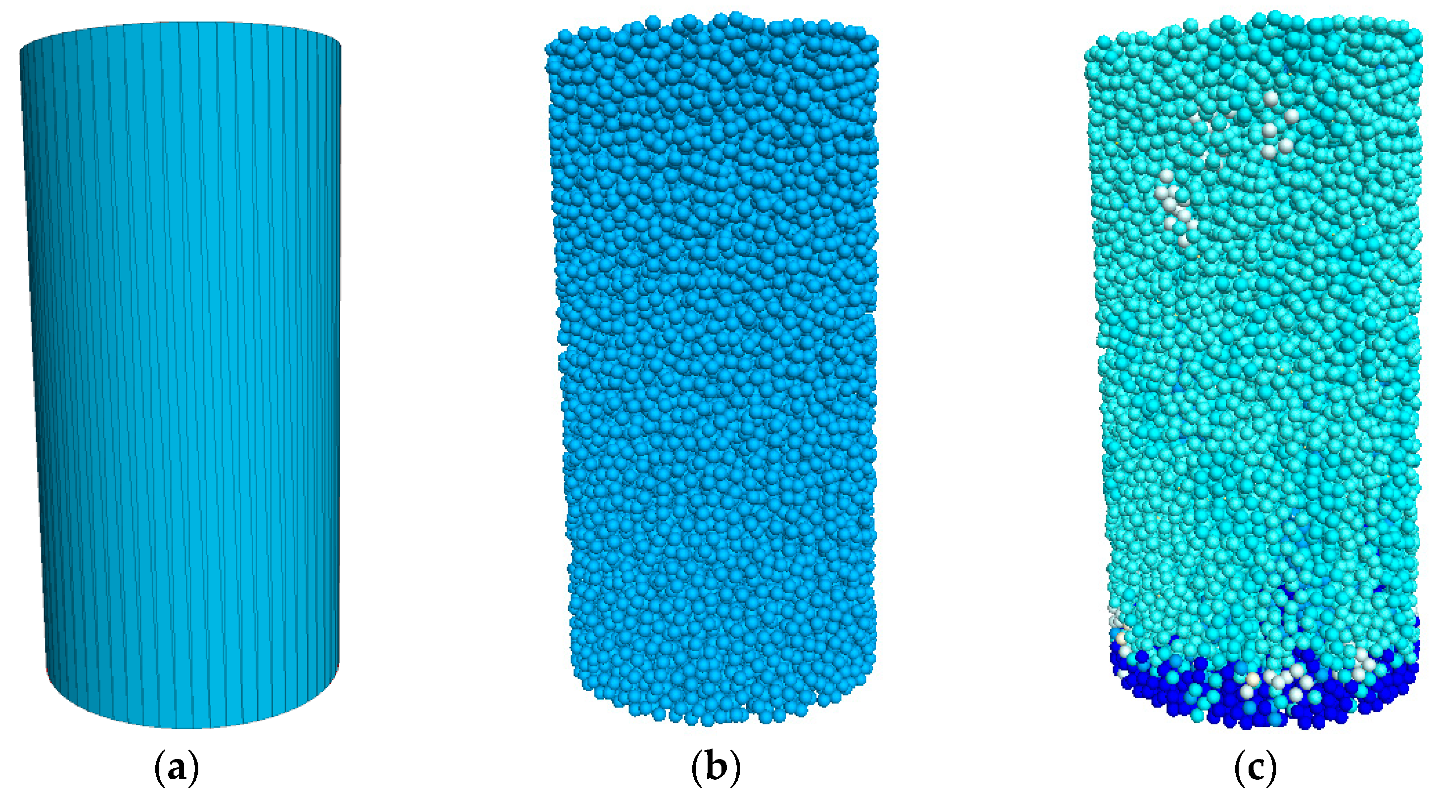
Based on the three gradation-controlling parameters (α, β, dmax) in Equation (2) and porosity (n) as variables, a total of 256 sets of CGS specimens were designed, with each variable set at four levels. Specifically, the parameter (α) was assigned values of 100, 200, 300, and 400; β took values of 2, 4, 6, and 8 × 10⁻⁴; dmax was set to 10, 20, 30, and 40 mm; and n varied as 0.1, 0.15, 0.20, and 0.25. The CFD-DEM simulations through PFC 6.0 (3D) were conducted to model permeability tests, determining the permeability coefficients for each specimen [39,40]. The primary procedures of the numerical simulation are as follows (see Figure 1):
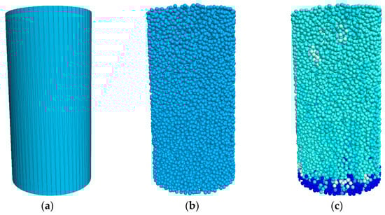
Figure 1.
Modeling using the CFD-DEM coupling method. (a) Cylindrical space generation; (b) Sample particle generation; (c) Seepage field application.
- Numerical model construction and CGS specimen generation
The first step involves defining the geometric dimensions of the test specimen, which is typically set as a cylindrical specimen with a diameter of 300 mm and a height of 600 mm. This configuration ensures sufficient representativeness while minimizing boundary effects. Either rigid or periodic boundaries can be applied to simulate realistic particle movement under seepage flow. Subsequently, CGS specimens are generated based on the prescribed gradation characteristics, either by employing an exponential continuous gradation equation or by directly importing experimental gradation data to ensure that the particle distribution adheres to the target gradation curve. The specimen is generated using the deposition method, where particles progressively fill the designated test region. After particle generation, gravitational settling is applied, followed by equivalent compaction, to achieve adequate particle contact and establish a stable pore structure. The initial porosity is then adjusted to approximate the target value, providing a reasonable initial state for subsequent seepage simulations.
- 2.
- CFD fluid domain definition and computational grid generation
The computational fluid dynamics (CFD) domain is first defined to align with the geometric boundaries of the CGS specimen. Suitable fluid boundary conditions are then imposed, such as applying a constant hydraulic head at the top and specifying either a fixed pressure or a free drainage boundary at the bottom to replicate actual seepage conditions. Next, the fluid domain is discretized using a computational grid, typically employing either a uniform cubic mesh or an adaptive meshing strategy. The grid size is selected to be compatible with particle dimensions, usually matching the smallest particle diameter to capture fluid–solid interface characteristics accurately. Once the meshing process is completed, the porosity of each grid element is calculated, and the fluid–solid coupling relationship is established to ensure the accuracy of the CFD computation. The fluid properties, including dynamic viscosity and density, are then defined. Fluid motion within the CGS medium is described using the Navier–Stokes equations to capture seepage flow behavior. The detailed meso-mechanical parameters in the numerical seepage simulations are presented in Table 1.

Table 1.
Meso-mechanical parameters in the numerical seepage simulation.
- 3.
- Seepage test simulation and data analysis
The seepage boundary conditions are initially imposed in the simulation of the seepage test. A constant hydraulic head or a constant flow rate is applied at the top, allowing fluid to infiltrate the CGS medium, while the bottom boundary is subjected to either a fixed pressure or a free drainage condition to ensure a steady seepage state. Once steady-state seepage is established, the pressure gradient and local flow velocity distribution within the specimen are monitored. The overall permeability coefficient is then computed based on Darcy’s law, providing quantitative insight into the seepage behavior of the CGS material.
The permeability coefficients of some specimens obtained through simulation are demonstrated in Table 2.
Table 2.
Partially derived datasets from CFD-DEM simulation of seepage tests.
3.2. Correlation Analysis
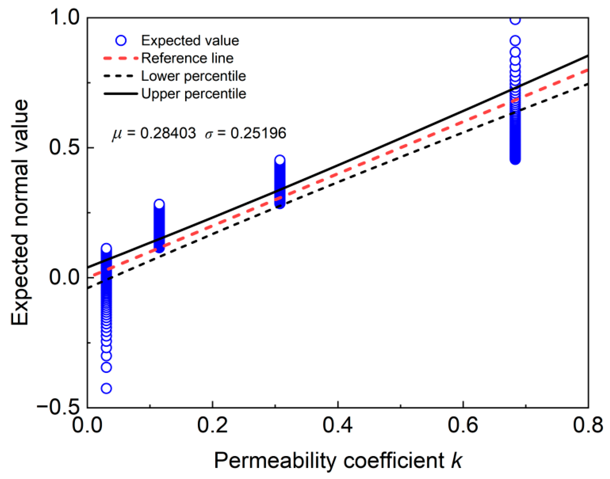
The relationships between the four input parameters (i.e., α, β, dmax, and n) and the output parameter (i.e., k) remain unclear. Directly inputting input parameters that influence the output parameter into the predictive model may obscure the effects of the dominant input parameters and increase the complexity of model training. Therefore, identifying the dominant input parameters can reduce the dimensionality of the sample space while enhancing model training efficiency. Grey relational analysis (GRA), a statistical method for multi-factor analysis, evaluates the degree of correlation between sequences based on the similarity of their curve shapes. The closer the curves, the stronger the correlation between the corresponding sequences, and vice versa. Accordingly, GRA can be employed to determine the dominant input parameters affecting the output parameter. As demonstrated in Figure 2, the grey relational coefficients (R) between each input parameter and k are as follows: 0.602 (α), 0.693 (β), 0.745 (dmax), and 0.842 (n), respectively. Generally, a grey relational coefficient (R > 0.6) indicates a strong correlation [41], suggesting that all four input parameters can be considered dominant parameters. Consequently, dimensionality reduction is not required.
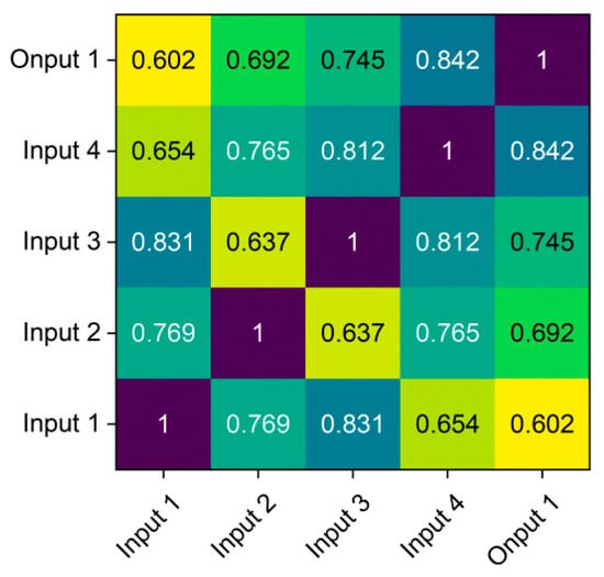
Figure 2.
Analysis of dominant input parameters based on the GRA algorithms.
3.3. Data Preprocessing
The 256 data sets obtained from this experiment were preprocessed to ensure that data quality met the requirements for modeling. The quantile–quantile plots of observed variables (see Figure 3) indicated a non-normal distribution, specifically, the expected normal values do not entirely fall within the 95% confidence interval. Thus, the interquartile range (IQR) method was intended for outlier detection. The IQR [42], defined as the difference between the 75th percentile (Q3) and the 25th percentile (Q1), serves as a measure of data dispersion. Outliers were identified as data points falling below (Q1 − 1.5 × IQR) or exceeding (Q3 + 1.5 × IQR). As demonstrated in Figure 4, no outliers were detected among the 256 data sets, confirming their suitability for subsequent analysis.

Figure 3.
Quantile–quantile plots of out parameter.
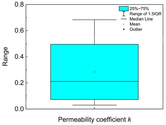
Figure 4.
Results of outlier detection.
4. Machine Learning Methodology
4.1. Machine Learning Algorithm
Three typical machine learning prediction algorithms (see Figure 5) were employed to analyze the permeability coefficient (k): a neural network model, the Back-Propagation Neural Network (BPNN) [43]; a machine learning regression model, Gaussian Process Regression (GPR) [44]; and a machine learning tree model, Random Forest (RF) [45]. BPNN is a multilayer feed-forward neural network based on gradient descent, wherein the training process optimizes network weights and biases via the back-propagation algorithm. Specifically, this algorithm computes the error at the output layer and propagates it backward through the network, adjusting the weights layer by layer. GPR, a regression model grounded in Bayesian theory, is particularly suited for predicting continuous outputs. It assumes that the data follow a Gaussian distribution and models the covariance matrix of the training data to infer predictions at unknown points along with their associated uncertainties. The critical component of GPR is the kernel function, which quantifies the similarity between data points. RF, an ensemble learning algorithm, constructs multiple decision trees based on randomly selected subsets of training data and features; the final prediction is then obtained by aggregating individual tree outputs, via voting for classification tasks or averaging for regression tasks [46]. Note: The above three machine learning algorithms are implemented by Matlab R2018a software.
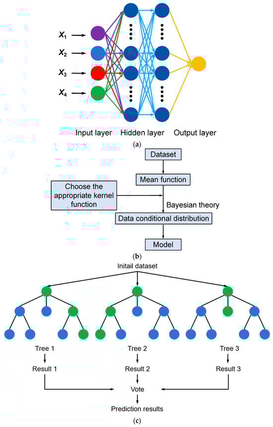
Figure 5.
Schematic diagram of permeability coefficient based on data-driven machine learning methods. (a) Back-Propagation Neural Network, BPNN; (b) Gaussian Process Regression, GPR; (c) Random Forest, RF.
4.2. Model Training and Optimization
4.2.1. Hyperparameter Optimization
Hyperparameter optimization is critical for enhancing the performance and generalizability of machine learning models. Unlike model parameters, which are learned during training, hyperparameters are preset and govern key aspects such as the learning rate, model complexity, and regularization. Appropriate tuning of these hyperparameters can effectively prevent overfitting, accelerate convergence, and improve the model’s robustness across diverse datasets. Consequently, through hyperparameter optimization, models can achieve more accurate and stable performance on complex tasks, thereby enhancing their applicability in practical scenarios.
A common approach to hyperparameter optimization involves the use of the particle swarm optimization (PSO) algorithm. Compared to directly employing machine learning models for prediction, the integration of PSO significantly enhances the global search capability for optimal model parameters, thereby improving prediction accuracy and reducing the risk of overfitting. Moreover, the PSO optimization process is model-independent, making it broadly applicable to various machine learning algorithms with strong generalizability. PSO mimics the search behavior of particles within the solution space to identify the optimal combination of hyperparameters. In the context of machine learning, hyperparameter optimization is a crucial step for improving model performance; PSO is particularly effective for global optimization over a broad search space, thereby avoiding the local optima often encountered with traditional grid or random search methods. PSO is an optimization technique inspired by the foraging behavior of bird flocks, where a population of particles collaborates by flying through the solution space to locate the global optimum. In this algorithm, each particle represents a potential solution and explores the space by updating its position and velocity. The velocity update is determined by a combination of inertia weight, the particle’s individual best-known position (pBest), and the global best-known position (gBest). Through iterative adjustments of particle velocities and positions, the swarm gradually converges to the optimal solution, as described in Equations (3) and (4).
where vi(t) represents the velocity of particle i at time t, while xi(t) denotes the corresponding position; pBesti is the individual best position achieved by particle i, and gBest is the global best position found across the entire swarm; the inertia weight w controls the influence of the previous velocity on the current update, whereas the learning factors c1 and c2 regulate the contributions of the individual best and global best positions, respectively; r1 and r2 are random numbers drawn from a uniform distribution over the interval [0, 1].
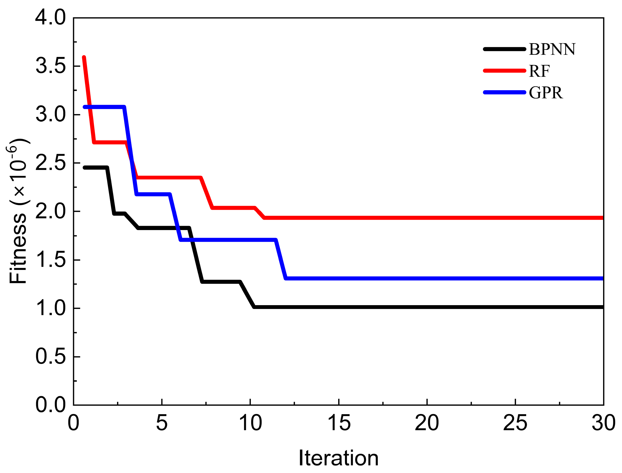
The variation in fitness values during the hyperparameter optimization of each machine learning model using the PSO algorithm is illustrated in Figure 6. As shown, the fitness values of all models decrease significantly through iterative optimization and tend to stabilize before the 13th generation. Among them, the BPNN model exhibits the lowest fitness value, suggesting its potential superiority over the other models. Upon completion of the iterations, the optimal hyperparameters for each machine learning model are retained and reintroduced into the respective models for subsequent selection of the optimal machine learning model.
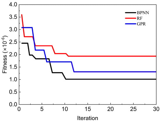
Figure 6.
Variation of fitness values for each model with the number of iterations.
4.2.2. Cross-Validation
A total of 256 data samples were randomly and uniformly divided into four groups, with three groups (75%) allocated for training and one group (25%) reserved for testing. To ensure the predictive model’s validity and generalizability and to mitigate overfitting, cross-validation was performed. In each cycle of model development and evaluation, a different group was designated for validation while the remaining groups were used for training. This process was repeated four times, and the final accuracy was determined by averaging the accuracies obtained from each of the four validation rounds.
4.3. Evaluation Metrics
In this investigation, a multidimensional evaluation framework was established using the coefficient of determination (R2), root mean square error (RMSE), mean absolute error (MAE), and 95% uncertainty interval width (U95) to systematically assess the model’s fitting capability and predictive accuracy. R2 quantifies the extent to which the model explains the variability of the target variable, thereby statistically reflecting the congruence between the model and the data distribution; its range of [0, 1] provides a standardized basis for comparing models across different scales. RMSE amplifies larger deviations through the squaring operation, thus accentuating the model’s sensitivity to outliers, while its dimensional consistency with the original data intuitively conveys the physical significance of the prediction error. In contrast, MAE, through linear computation, evenly weighs the error contributions of individual samples, offering a more robust accuracy assessment in the presence of outliers. Together, these metrics complement one another: R2 emphasizes the overall ability of the model to capture data trends, RMSE underscores the impact of significant deviations, MAE reflects the stability of the model’s predictions, and U95 measures the prediction stability and reliability of different models or the same model under different input conditions. The combined analysis not only reveals the model’s theoretical explanatory power but also enables a multidimensional diagnosis of its error characteristics in practical applications, thereby providing directional guidance for further model optimization. The details for evaluation metrics are demonstrated in Table 3.
Table 3.
Prediction performance assessment system.
5. Results and Discussion
5.1. Comparison of Model Performance
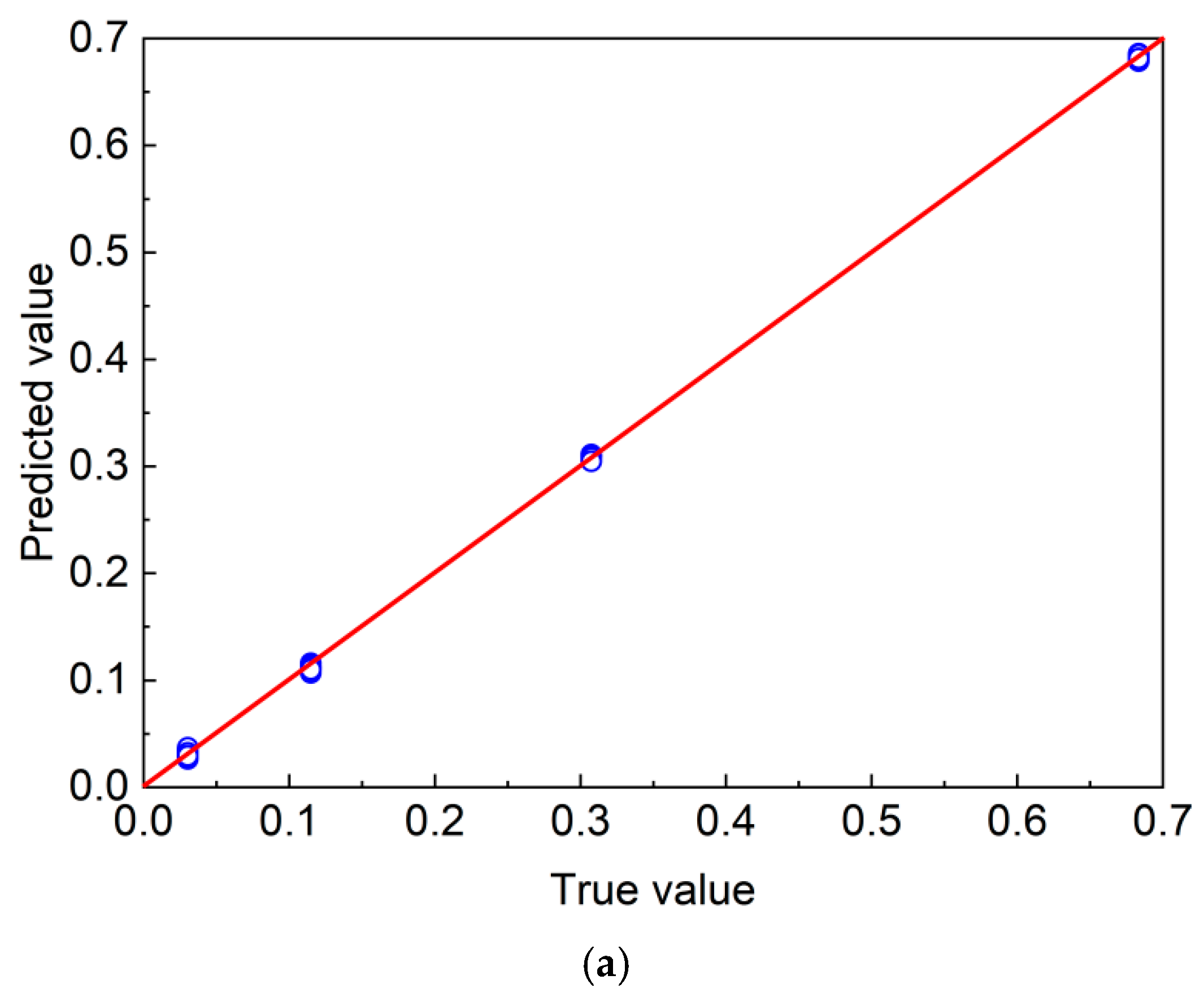
The prediction results (the 4th training) on the test set for each model are presented in Figure 7. The BPNN, GPR, and RF models yielded satisfactory predictions of the permeability coefficient, with the data points largely distributed around the 45° line, indicating strong agreement between the predicted and observed values.
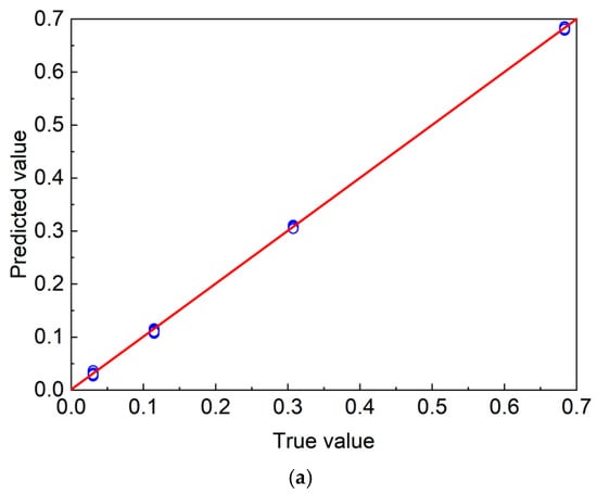
Figure 7.
Predictive performance of machine learning models in the testing dataset (the 4th training). (a) BPNN; (b) GPR; (c) RF.
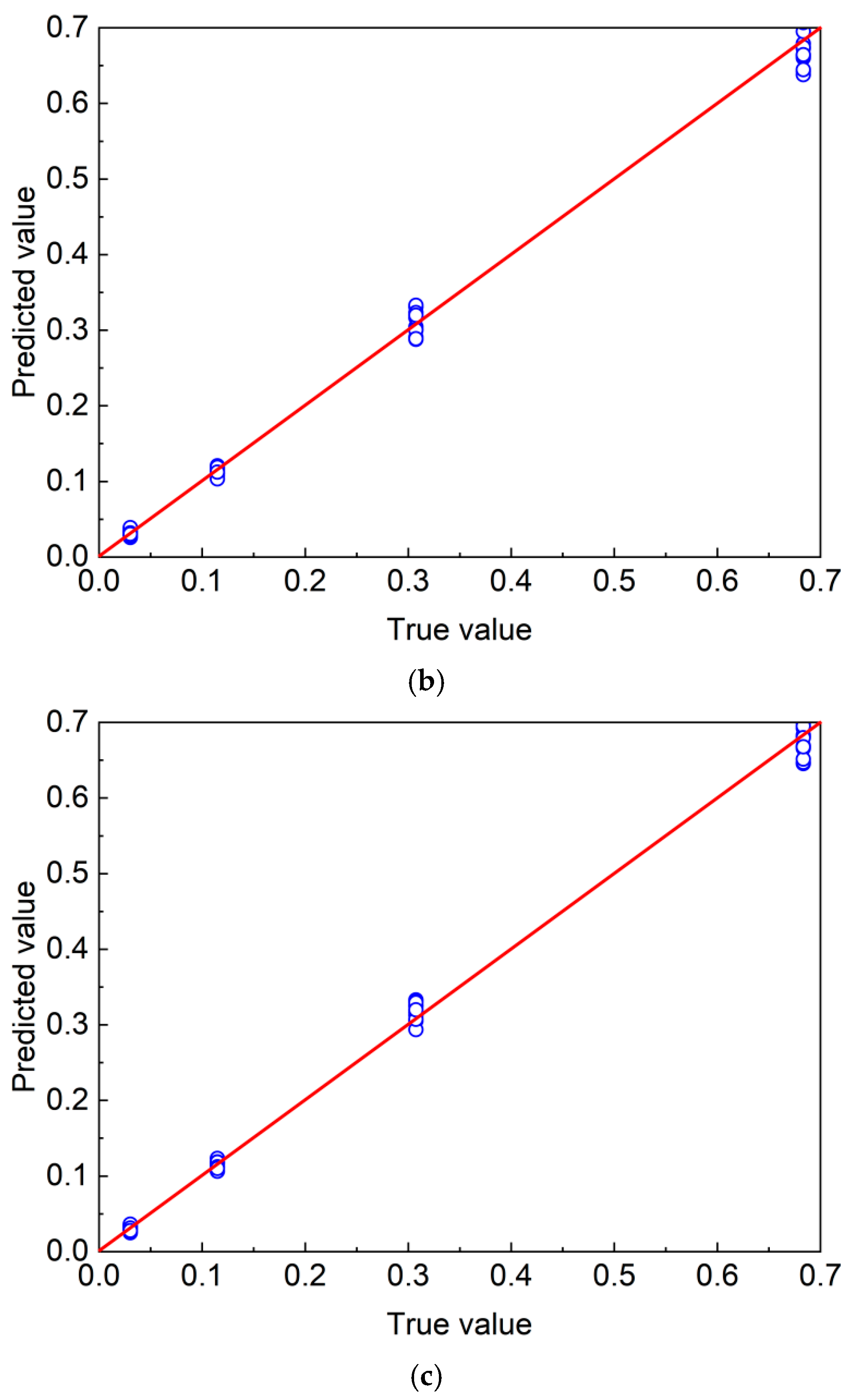
The three models exhibited significant differences in predicting the permeability coefficient of coarse-grained soils, as evidenced by the cross-validation results (see Figure 8). The BPNN demonstrated the best overall performance, achieving an average (R2) as high as 0.99 and mean absolute error (MAE), root mean square error (RMSE), and 95% uncertainty interval width (U95) values of only 1.5, 2.9, and 0.4, respectively. These metrics indicate that BPNN possesses a high degree of fit to the data characteristics and exhibits extremely low prediction bias, thereby capturing the complex nonlinear relationships between the permeability coefficient and the input parameters effectively. Its superior performance may be attributed to its deep feature extraction capabilities, which characterize high-order interactions among critical factors such as particle gradation and pore structure effectively.
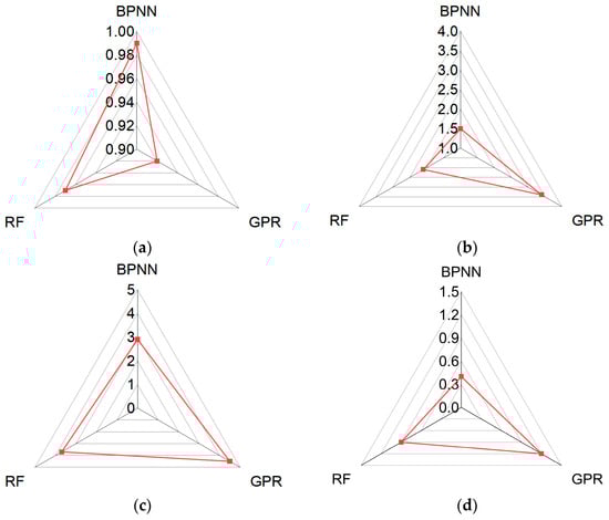
Figure 8.
Evaluation metrics results of machine learning models in the testing dataset. (a) R2; (b) MAE; (c) RMSE; (d) U95.
In contrast, GPR exhibited relatively lower predictive accuracy, with an (R2) of 0.92, MAE of 3.4, RMSE of 4.5, and U95 of 1.2. This reduced performance may be associated with the selection of its kernel function and suboptimal parameter tuning. The noise sensitivity inherent in GPR becomes problematic when processing coarse-grained soil permeability data, particularly when experimental measurements include errors or the sample distribution is uneven. Moreover, potential threshold effects in permeability prediction, such as those arising from a critical void ratio, may not be well accommodated by the default Gaussian assumptions in GPR, thereby diminishing its ability to predict extreme values accurately.
The performance of the RF model fell between the two, with an (R2) of 0.97, MAE of 2.1, RMSE of 3.7, and U95 of 0.9. RF maintained high accuracy and exhibited robust performance, owing to its ensemble of decision trees. This behavior can be attributed to the inherent compatibility between the piecewise linear relationships of the permeability coefficient with the feature variables and the decision tree’s splitting mechanism. However, compared with BPNN, the noticeable differences in MAE, RMSE, and U95 suggest that tree-based models may still face limitations in regression tasks when capturing subtle variations in continuous permeability coefficients, likely due to an insufficient level of smoothness [47].
5.2. Evaluation Against Traditional Methods
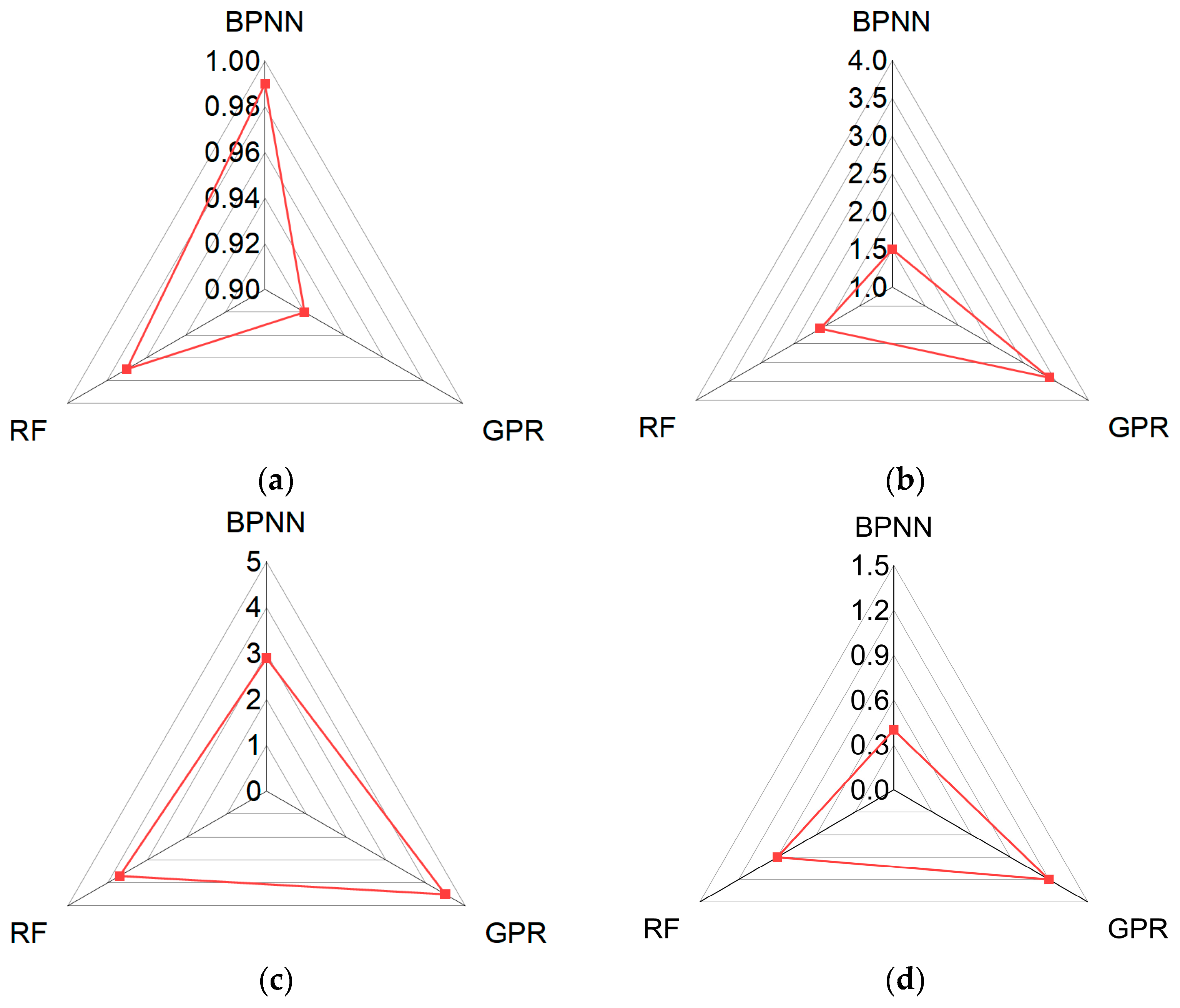
In summary, the BPNN model demonstrated the best overall performance in predicting the permeability coefficient of CGSs. To further highlight the advantages of the BPNN model over traditional empirical models, this section compares its predictive performance with the empirical model proposed by [48] (see Equation (5)), which was derived based on the negative exponential continuous gradation equation. The comparison is conducted using the permeability test datasets from [48,49] (detailed as Table 4 and Table 5), providing a comprehensive evaluation of the predictive capabilities of both models (see Figure 9 and Table 6).
Table 4.
Parameters of negative exponential grading equation and porosity derived from [48].
Table 5.
Parameters of negative exponential grading equation and porosity derived from [49].
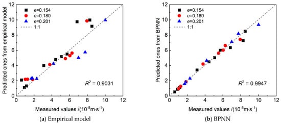
Figure 9.
Comparison of the prediction results for CGS permeability coefficients between empirical model and a BPNN model [49]. (a) Empirical model; (b) BPNN.
Table 6.
Comparison of the prediction results for CGS permeability coefficients between empirical model and a BPNN model [48].
For the case derived from [48], the relative error δ of the empirical model ranges from 2.0–88.3%, whereas that of the BPNN model ranges from 1.5–19.4%, demonstrating the great stability. For the case derived from [49], prediction accuracy analysis revealed that the empirical model achieved a coefficient of determination of R2 = 0.9031, whereas the BPNN model attained R2 = 0.9947, marking a 10.13% improvement. This enhancement indicates that the BPNN model, through its nonlinear mapping mechanism, more precisely captures the complex relationship between gradation parameters and permeability coefficients, with its fitted curve exhibiting a significantly better alignment with the experimental data than traditional empirical formulas. The data-driven approach demonstrated consistently high precision on both the training and validation sets, overcoming the inherent biases imposed by theoretical assumptions in empirical models and providing a more reliable predictive tool for evaluating the permeability of coarse-grained soils.
6. Conclusions
In this investigation, CGS specimens were designed using a negatively exponential continuous gradation equation, and a permeability coefficient database was constructed by integrating CFD-DEM simulated seepage tests. The predictive performance of three machine learning models—Back-Propagation Neural Network (BPNN), Gaussian Process Regression (GPR), and Random Forest (RF)—was systematically compared with that of traditional empirical models. Grey relational analysis (GRA) was employed to quantify the contribution of input parameters, while particle swarm optimization (PSO) combined with four-fold cross-validation enhanced the models’ generalization capability, thereby demonstrating the advantages of data-driven methods in evaluating the permeability of coarse-grained soils. The main conclusions are summarized as follows:
- (1)
- Grey relational analysis revealed that the gradation parameters α, β, maximum particle size (dmax), and porosity (n) significantly influence the permeability coefficient (grey relational coefficient R > 0.6). Consequently, these four parameters should be jointly employed as input variables, obviating the need for dimensionality reduction.
- (2)
- Among the models evaluated, BPNN achieved superior accuracy (R2 = 0.99, MAE = 1.5, RMSE = 2.9, U95 = 0.4), demonstrating its robust nonlinear mapping capability to accurately capture higher-order interactions affecting the permeability coefficient. In contrast, GPR exhibited the lowest accuracy (R2 = 0.92) due to limited kernel adaptability and noise sensitivity, while RF (R2 = 0.97) encountered challenges in modeling the smooth variations of continuous variables.
- (3)
- Compared to the traditional empirical model (R2 = 0.9031), the BPNN’s predictive accuracy improved by 10.13%, with high consistency observed between training and validation results. These findings confirm that data-driven methods effectively overcome the limitations imposed by theoretical assumptions and enhance the reliability of permeability assessments for coarse-grained soils, offering an efficient solution for the intelligent prediction of geotechnical parameters.
The innovation of this study lies in the integration of CFD-DEM simulated datasets based on negatively exponential continuous gradation to capture realistic seepage behavior of coarse-grained soils, combined with the use of grey relational analysis to ensure the physical interpretability and relevance of input variables. Furthermore, a particle swarm optimization (PSO) strategy coupled with k-fold cross-validation was implemented to enhance the generalization capability of machine learning models. The systematic comparison of BPNN, RF, and GPR further reveals the superior performance of BPNN in modeling complex nonlinear relationships, offering a more accurate and data-efficient approach for permeability prediction than existing empirical or machine learning methods.
Limitations and Future Scopes
Despite the promising results achieved in this study, several limitations should be acknowledged. First, the permeability coefficient database was derived entirely from CFD-DEM simulations, which, although capable of capturing pore-scale flow behavior, may not fully replicate the heterogeneity and boundary conditions of real-world CGSs. Second, the model inputs were limited to gradation parameters and porosity; other potentially influential factors such as particle shape, angularity, and fabric structure were not considered. Moreover, the machine learning models were trained and validated on a relatively constrained parameter space, which may limit their generalizability when extrapolated to soils with markedly different gradation characteristics. Future research should focus on incorporating experimental datasets to validate and enhance the robustness of the predictive models, exploring additional microstructural descriptors as input features, and extending the framework to accommodate dynamic seepage conditions or coupled hydro-mechanical processes for broader geotechnical applications.
Author Contributions
Conceptualization, J.W. and H.D.; methodology, J.W.; software, L.G.; validation, J.W., H.D. and L.G.; formal analysis, J.W.; investigation, J.W.; resources, Y.W.; data curation, Y.W.; writing—original draft preparation, Y.W.; writing—review and editing, Y.W.; visualization, J.W.; supervision, J.W.; project administration, J.W.; funding acquisition, J.W. All authors have read and agreed to the published version of the manuscript.
Funding
This investigation was funded by the National Key R&D Program of China (No. 2023YFC3009400); the National Science Fund of Jiangxi Province (No. 20223BBG71018); Fujian Natural Science Foundation (No. 2021J011134); Science and Technology Innovation Development Fund of Wuyi University (No. N2017Y05); Engineering Research Center of Prevention and Control of Geological Disasters in Northern Fujian, Fujian Province University (No. WYERC2024-4).
Data Availability Statement
Data will be made available on request.
Conflicts of Interest
The authors declare that they have no known competing financial interests.
Nomenclature
| α, β | Fitting parameters in the negative exponential gradation equation (NEGE). α controls the shape of the gradation curve, and β controls the degree of inclination. |
| d | Particle diameter (mm), the independent variable in the gradation equation. |
| dmax | Maximum particle diameter (mm), a parameter in the gradation equation. |
| P | Percentage of soil mass smaller than a given particle size. |
| n | Porosity, the ratio of the volume of pores to the total volume of soil. |
| k | Permeability coefficient, a key parameter measuring the seepage ability of soil. |
| Cᵤ | Uniformity coefficient, reflecting the uniformity of particle size distribution. |
| Cc | Curvature coefficient, reflecting the shape of the gradation curve (e.g., smoothness or abruptness of particle size transitions). |
| BPNN | Back-Propagation Neural Network, a multi-layer feedforward neural network based on gradient descent, optimizing weights and biases via back-propagation. |
| GPR | Gaussian Process Regression, a Bayesian-based regression model suitable for continuous output prediction, modeling the covariance of data to infer predictions and uncertainties. |
| RF | Random Forest, an ensemble learning algorithm constructing multiple decision trees from random subsets of data/features, aggregating results via averaging for regression. |
| R2 | Coefficient of determination, measuring how well the model explains the variance of the target variable (closer to 1 indicates better fit). |
| RMSE | Root Mean Square Error, quantifying the average magnitude of prediction errors (dimensional consistency with the target variable). |
| MAE | Mean Absolute Error, averaging absolute differences between predictions and true values (robust to outliers). |
| U95 | 95% Uncertainty Interval Width, the width of the 95% confidence interval for predictions, indicating the stability of model outputs (smaller values mean more reliable predictions). |
| CFD-DEM | Computational Fluid Dynamics–Discrete Element Method, a coupled simulation technique modeling fluid–particle interactions in seepage flow, combining CFD for fluid dynamics and DEM for particle mechanics. |
| PSO | Particle Swarm Optimization, an algorithm mimicking swarm behavior to optimize hyperparameters. Key variables in PSO |
| GRA | Gray Relational Analysis, a statistical method evaluating correlations between factors by measuring the similarity of their curve shapes. |
References
- Ding, X.-H.; Luo, B.; Zhou, H.-T.; Chen, Y.-H. Generalized solutions for advection–dispersion transport equations subject to time- and space-dependent internal and boundary sources. Comput. Geotech. 2025, 178, 106944. [Google Scholar] [CrossRef]
- Chen, Y.; Zhang, L.; Xu, L.; Zhou, S.; Luo, B.; Ding, K. In-situ investigation on dynamic response of highway transition section with foamed concrete. Earthq. Eng. Eng. Vib. 2025, 2025, 1–17. [Google Scholar] [CrossRef]
- Yilmaz, I.; Marschalko, M.; Bednarik, M.; Kaynar, O.; Fojtova, L. Neural computing models for prediction of permeability coefficient of CGSs. Neural Comput. Appl. 2012, 21, 957–968. [Google Scholar] [CrossRef]
- Indrawan, I.G.B.; Rahardjo, H.; Leong, E.C. Effects of coarse-grained materials on properties of residual soil. Eng. Geol. 2006, 82, 154–164. [Google Scholar] [CrossRef]
- Bao, M.-D.; Zhu, J.-G.; Zheng, H.-F.; Liu, Z. Influence of Gradation of Coarse-Grained Soil on the Permeability Coefficient. Soil Mech. Found. Eng. 2021, 58, 367–373. [Google Scholar] [CrossRef]
- Wang, K.; Tang, L.; Tian, S.; Ling, X.; Cai, D.; Liu, M. Experimental investigation and prediction model of permeability in solidified coarse-grained soil under freeze-thaw cycles in water-rich environments. Transp. Geotech. 2023, 41, 101035. [Google Scholar] [CrossRef]
- Nguyen, B.T.; Ishikawa, T.; Murakami, T. Effects evaluation of grass age on hydraulic properties of coarse-grained soil. Transp. Geotech. 2020, 25, 100401. [Google Scholar] [CrossRef]
- Zhai, Q.; Rahardjo, H.; Satyanaga, A.; Dai, G. Estimation of the soil-water characteristic curve from the grain size distribution of coarse-grained soils. Eng. Geol. 2020, 267, 105502. [Google Scholar] [CrossRef]
- Zhang, X.; Wei, Y.; Tu, G.; Yang, H.; Zhang, S.; Liang, P. Darcy to non-Darcy seepage transition in heterogeneous coarse-grained soil: Seepage characteristics and critical threshold prediction. J. Rock Mech. Geotech. Eng. 2024, 17, 2526–2538. [Google Scholar] [CrossRef]
- Fan, D.; Zhang, C.; Ji, Y.; Zhao, X.; Zhao, Z.; He, M. Permeability Evolution of Rough Fractures in Gonghe Granite Subjected to Cyclic Normal Stress at Elevated Temperatures: Experimental Measurements and Analytical Modeling. Rock Mech. Rock Eng. 2024, 57, 11301–11318. [Google Scholar] [CrossRef]
- Yang, B.; Xu, T.; Du, Y.; Jiang, Z.; Tian, H.; Yuan, Y.; Zhu, H. Numerical investigation on the influence of CO2-induced mineral dissolution on hydrogeological and mechanical properties of sandstone using coupled lattice Boltzmann and finite element model. J. Hydrol. 2024, 639, 131616. [Google Scholar] [CrossRef]
- Wei, C.; Li, Y.; Liu, X.; Zhang, Z.; Wu, P.; Gu, J. Large-scale application of coal gasification slag in nonburnt bricks: Hydration characteristics and mechanism analysis. Constr. Build. Mater. 2024, 421, 135674. [Google Scholar] [CrossRef]
- Liu, H.; Wang, J.; Abiyasi; Li, H.; Yin, C.; Liu, J.; Chen, G. Effect of Coal Gasification Slag on Improving Physical Properties of Acid Soil. Sci. Adv. Mater. 2022, 14, 703–709. [Google Scholar] [CrossRef]
- Lee, H.-H.; Hsu, C.-F.; Chao, S.-J.; Chi, C.-C. A Study on the Reasons for No Soil Liquefaction Occurring in the Lanyang Plain in a Strong Earthquake Area. Sustainability 2022, 14, 8244. [Google Scholar] [CrossRef]
- Wang, T.-L.; Zhang, Y.-Z.; Shu, Y.; Feng, Z.-X.; Yue, Z.-R. Liquid water–vapour migration tracing and characteristics of coarse-grained soil under high-speed railway train loading in cold regions. Cold Reg. Sci. Technol. 2021, 187, 103283. [Google Scholar] [CrossRef]
- Yao, M.; Wang, H.; Yu, Q.; Li, H.; Xia, W.; Wang, Q.; Huang, X.; Lin, J. Anisotropy Study on the Process of Soil Permeability and Consolidation in Reclamation Areas: A Case Study of Chongming East Shoal in Shanghai. Buildings 2023, 13, 3059. [Google Scholar] [CrossRef]
- Taslimian, R.; Noorzad, A. Liquefaction Mitigation Using Stone Columns with Non-Darcy Flow Theory. Geotech. Geol. Eng. 2024, 42, 4375–4399. [Google Scholar] [CrossRef]
- Guo, Z.; Liu, Y.; Zhang, T.; Zhang, J.; Wang, H.; He, J.; Li, G.; Tian, B. Revealing the Effect of Typhoons on the Stability of Residual Soil Slope by Wind Tunnel Test. Forests 2024, 15, 791. [Google Scholar] [CrossRef]
- Horak, E.; Komba, J.; Maina, J.; Sebaaly, H. Contiguous Aggregate Packing as Common Principle for Asphalt Density, Strength and Permeability Control. SSRN Strength Permeability Control 2021. preprint. [Google Scholar] [CrossRef]
- Wang, T.-L.; Zhang, F.; Wang, Y.; Wu, Z.; He, Y.-M.; Yue, Z.-R. Experimental Study on Temperature Field Evolution Mechanism of Artificially Frozen Gravel Formation under Groundwater Seepage Flow. Adv. Mater. Sci. Eng. 2022, 2022, 8940816. [Google Scholar] [CrossRef]
- Bai, H.; Feng, W.; Yi, X.; Fang, H.; Wu, Y.; Deng, P.; Dai, H.; Hu, R. Group-occurring landslides and debris flows caused by the continuous heavy rainfall in June 2019 in Mibei Village, Longchuan County, Guangdong Province, China. Nat. Hazards 2021, 108, 3181–3201. [Google Scholar] [CrossRef]
- Fidan, A.A.; Berilgen, M.M. Drainage Characteristics, Capillary Barrier Effect, and Diversion Length of Flat Earthen Roof of Historical Kemaliye Houses. Int. J. Arch. Herit. 2024, 2024, 1–23. [Google Scholar] [CrossRef]
- Li, X.; Zhang, K.; Bao, K.; Zhao, J.; Wang, X.; Tang, Y. Effect of coal gasification coarse slag on soil water and nutrition at an arid opencast coal mine site in Northwest China. Land Degrad. Dev. 2024, 35, 3112–3125. [Google Scholar] [CrossRef]
- Jin, Z.; Tang, S.; Yuan, L.; Xu, Z.; Chen, D.; Liu, Z.; Meng, X.; Shen, Z.; Chen, L. Areal artificial recharge has changed the interactions between surface water and groundwater. J. Hydrol. 2024, 637, 131318. [Google Scholar] [CrossRef]
- Huang, B.; Guo, C.; Tang, Y.; Guo, J.; Cao, L. Experimental Study on the Permeability Characteristic of Fused Quartz Sand and Mixed Oil as a Transparent Soil. Water 2019, 11, 2514. [Google Scholar] [CrossRef]
- Hu, J.; Chen, B.; Chu, X.; Gong, H.; Zhou, C.; Yang, Y.; Sun, X.; Zhao, D. Simulation and prediction of land subsidence in Decheng District under the constraint of InSAR deformation information. Front. Earth Sci. 2024, 12, 1458416. [Google Scholar] [CrossRef]
- Wu, Z.; Yang, S.; Liu, W.; Li, Y. Permeability analysis of gas hydrate-bearing sand/clay mixed sediments using effective stress laws. J. Nat. Gas Sci. Eng. 2022, 97, 104376. [Google Scholar] [CrossRef]
- Kinslev, E.M.; Hededal, O.; Rocchi, I.; Zania, V. Primary and secondary consolidation characteristics of a high plasticity overconsolidated clay in compression and swelling. Soils Found. 2023, 63, 101375. [Google Scholar] [CrossRef]
- Khanh, P.T.; Pramanik, S.; Ngoc, T.T.H. Soil Permeability of Sandy Loam and Clay Loam Soil in the Paddy Fields in An Giang Province in Vietnam. Environ. Chall. 2024, 15, 100907. [Google Scholar] [CrossRef]
- Zhao, L.; Tian, W.; Liu, K.; Yang, B.; Guo, D.; Lian, B. An empirical relationship of permeability coefficient for soil with wide range in particle size. J. Soils Sediments 2024, 24, 2926–2937. [Google Scholar] [CrossRef]
- Gao, M.Y.; Ji, F.; Hong, Z.-S.; Shi, X.S. Changing law of permeability coefficient during compression for reconstituted sandy clays. Mar. Georesour. Geotechnol. 2023, 42, 1651–1659. [Google Scholar] [CrossRef]
- Zeybek, A.; Madabhushi, G.S.P. Assessment of soil parameters during post-liquefaction reconsolidation of loose sand. Soil Dyn. Earthq. Eng. 2023, 164, 107611. [Google Scholar] [CrossRef]
- Peng, J.; Shen, Z.; Zhang, W.; Song, W. Deep-Learning-Enhanced CT Image Analysis for Predicting Hydraulic Conductivity of Coarse-Grained Soils. Water 2023, 15, 2623. [Google Scholar] [CrossRef]
- Gulaly, L.; Luqman, M.; Usman, H.; Aziz, A.; Yousafzai, M.G.; Khan, K.; Khan, M. Predicting coefficient of permeability of soils: An interpretable machine learning approach augmented by deep generative adversarial network. Multiscale Multidiscip. Model. Exp. Des. 2025, 8, 143. [Google Scholar] [CrossRef]
- Zhang, R.; Zhang, S. Coefficient of permeability prediction of soils using gene expression programming. Eng. Appl. Artif. Intell. 2024, 128, 107504. [Google Scholar] [CrossRef]
- Zhang, Y.; Hua, Y.; Zhang, X.; He, J.; Jia, M.; Cao, L.; An, Z. Enhancing stability and interpretability in the study of strength behavior for coarse-grained soils. Comput. Geotech. 2024, 171, 106333. [Google Scholar] [CrossRef]
- Pham, B.T.; Ly, H.-B.; Al-Ansari, N.; Ho, L.S. A Comparison of Gaussian Process and M5P for Prediction of Soil Permeability Coefficient. Sci. Program. 2021, 2021, 3625289. [Google Scholar] [CrossRef]
- Showkat, R.; Jalal, F.E.; Babu, G.L.S. Estimation of Soil Water Characteristic Curve Using Machine-Learning Algorithms and Its Application in Embankment Response. J. Comput. Civ. Eng. 2025, 39, 04025012. [Google Scholar] [CrossRef]
- Xing, L.; Gong, W.; Huang, J.; Zhang, H.; Xing, B.; Wang, L. An improved CFD-DEM coupling method for simulating the steady seepage-induced behaviors of soil-rock mixture slopes. Comput. Geotech. 2025, 180, 107069. [Google Scholar] [CrossRef]
- Chopra, S.; Sajjadi, B. A mechanistic analysis of particle flow in a pulsatile circulating dual fluidized bed for chemical looping technology based on CDF-DEM simulation. Powder Technol. 2023, 435, 107069. [Google Scholar] [CrossRef]
- Mao, X.; Cai, P.; Fu, J.; Dai, Z. Study on internal erosion and structural evolution mechanism of soil–rock mixture. Nat. Hazards 2023, 118, 1739–1764. [Google Scholar] [CrossRef]
- Tzeng, C.-J.; Lin, Y.-H.; Yang, Y.-K.; Jeng, M.-C. Optimization of turning operations with multiple performance characteristics using the Taguchi method and Grey relational analysis. J. Mech. Work. Technol. 2009, 209, 2753–2759. [Google Scholar] [CrossRef]
- Kang, S.J.; Lee, M. Q-convergence with interquartile ranges. J. Econ. Dyn. Control. 2005, 29, 1785–1806. [Google Scholar] [CrossRef]
- Cui, L.; Tao, Y.; Deng, J.; Liu, X.; Xu, D.; Tang, G. BBO-BPNN and AMPSO-BPNN for multiple-criteria inventory classification. Expert Syst. Appl. 2021, 175, 114842. [Google Scholar] [CrossRef]
- Solla, M.; Pérez-Gracia, V.; Fontul, S. A Review of GPR Application on Transport Infrastructures: Troubleshooting and Best Practices. Remote Sens. 2021, 13, 672. [Google Scholar] [CrossRef]
- Elbeltagi, A.; Pande, C.B.; Kumar, M.; Tolche, A.D.; Singh, S.K.; Kumar, A.; Vishwakarma, D.K. Prediction of meteorological drought and standardized precipitation index based on the random forest (RF), random tree (RT), and Gaussian process regression (GPR) models. Environ. Sci. Pollut. Res. 2023, 30, 43183–43202. [Google Scholar] [CrossRef]
- Su, Y.; Luo, B.; Luo, Z.; Xu, F.; Huang, H.; Long, Z.; Shen, C. Mechanical characteristics and solidification mechanism of slag/fly ash-based geopolymer and cement solidified organic clay: A comparative study. J. Build. Eng. 2023, 71, 106459. [Google Scholar] [CrossRef]
- Chen, Y.H.; Zhang, L.; Zhou, J.; Liu, Z.S. Predicting permeability coefficient in soil-rock mixtures using parameters from the negative exponential continuous grading equation. IOP Conf. Ser. Earth Environ. Sci. 2024, 1335, 012005. [Google Scholar] [CrossRef]
- Yang, Z.H.; Yue, Z.R.; Feng, H.P.; Ye, C.; Zhou, J.; Jie, S. Experimental study of permeability properties of graded macadam in heavy haul railway subgrade bed surface layer. Rock Soil Mech. 2021, 42, 193–202. [Google Scholar] [CrossRef]


Disclaimer/Publisher’s Note: The statements, opinions and data contained in all publications are solely those of the individual author(s) and contributor(s) and not of MDPI and/or the editor(s). MDPI and/or the editor(s) disclaim responsibility for any injury to people or property resulting from any ideas, methods, instructions or products referred to in the content. |
© 2025 by the authors. Licensee MDPI, Basel, Switzerland. This article is an open access article distributed under the terms and conditions of the Creative Commons Attribution (CC BY) license (https://creativecommons.org/licenses/by/4.0/).