Abstract
Fourier ptychographic microscopy (FPM) has recently emerged as an important non-invasive imaging technique which is capable of simultaneously achieving high resolution, wide field of view, and quantitative phase imaging. However, FPM still faces challenges in the image reconstruction due to factors such as noise, optical aberration, and phase wrapping. In this work, we propose a semi-supervised Fourier ptychographic transformer network (SFPT) for improved image reconstruction, which employs a two-stage training approach to enhance the image quality. First, self-supervised learning guided by low-resolution amplitudes and Zernike modes is utilized to recover pupil function. Second, a supervised learning framework with augmented training datasets is applied to further refine reconstruction quality. Moreover, the unwrapped phase is recovered by adjusting the phase distribution range in the augmented training datasets. The effectiveness of the proposed method is validated by using both the simulation and experimental data. This deep-learning-based method has potential applications for imaging thicker biology samples.
1. Introduction
Fourier ptychographic microscopy (FPM) [1] is an innovative computational imaging technique designed to address the challenge of achieving both a large field of view and high resolution, with which traditional microscopy techniques struggle to balance [2]. FPM achieves high space/bandwidth product and quantitative phase imaging without the precise mechanical scanning devices or the interferometric systems [3], offering a cost-effective solution with promising application potential [4]. However, conventional FPM methods suffer from image reconstruction issues such as low computational efficiency, susceptibility to noise, aberration effects and phase wrapping problem [5]. To address these challenges, various improvements have been proposed [6,7,8,9], including Wirtinger flow optimization [10] and the simulated annealing algorithm [11]. With the advancement of deep learning, its application in FPM has also seen widespread adoption [12,13,14,15,16].
Currently, the mainstream applications of deep learning in FPM can be categorized into two types. The first type leverages large training datasets to directly learn the mapping from low-resolution amplitude to high-resolution amplitude and phase [17]. Examples include convolutional neural network-based models like Ptychnet [18], along with subsequent improvements introduced by Zhang et al. [19], which incorporates multi-scale architectures, residual connections, attention mechanisms, and various other enhancements. F. Bardozzo et al. applied generative adversarial networks (GANs) to achieve high-resolution, artifact-free reconstructions with robust cross-explainability and clinical validation [20]. T. Feng et al. proposed a linear-space-variant (LSV) model to achieve uniform full-field imaging while effectively eliminating vignetting-induced artifacts without segmenting the images [21]. K. Wu et al. introduced a blind deep-learning-based preprocessing method (BDFP) that enhances noise robustness by modeling noise distribution for data augmentation [22]. These data-driven approaches achieve image reconstruction by learning complex mapping relationships, and most of them are supervised learning. Once trained, the rapid inference is allowed within the same experimental setup.
The second type integrates the physical imaging model as prior knowledge, forming a physics-guided neural network architecture [23]. For instance, Jiang et al. [24] and Zhang et al. [25] simulated the forward imaging process of FPM using a neural network, with high-resolution amplitude and phase images as trainable parameters. By using optimization algorithms like gradient descent, the network is trained by its low-resolution amplitude output data distribution, which matches the experimentally collected data distribution. Zhang et al. [26] incorporated a single iteration of the FPM forward algorithm as a data preprocessing step, using the neural network for subsequent optimization to reduce network complexity [27]. Wu et al. proposed the denoising diffusion probabilistic models for Fourier ptychography method [28], which combines diffusion models with Wirtinger gradient descent techniques, offering a new approach to FPM reconstruction. These physically guided methods typically do not require manual GT labels and can be considered self-supervised learning, offering the advantage of low-cost reconstruction; however, their parameter optimization process was often tailored to single sample, limiting the advantage of deep learning that can optimize results using large datasets.
When encountering phase wrapping problem that arise with samples exhibiting significant phase distribution differences, FPM typically employs physical methods or phase unwrapping algorithms to address the problem, such as introducing solutions with varying refractive indices into the sample. And traditional unwrapping algorithms tend to exhibit substantial reconstruction errors when dealing with complex phase structures [29,30]. The advancement of deep learning offers a novel approach to phase unwrapping in FPM [31].
Based on our previous work on a Fourier ptychographic transformer (FPT) [32], this paper further introduces a semi-supervised Fourier ptychographic microscopy method, inspired by two mainstream approaches in the application of deep learning to FPM, termed SFPT. Semi-supervised learning bridges the gap between supervise learning and self-supervise learning by leveraging both labeled and unlabeled data [33]. In this framework, unlabeled data, integrated with the forward imaging principles of FPM, provide additional learning signals such as pupil aberration to the labeled data, thereby improving model performance. We utilize self-supervised learning to reconstruct pupil aberration parameters of the Zernike model from real datasets. Considering the detrimental effects of information loss and the inherent noise during the forward downsampling process, relying only on the captured low-resolution amplitude images as a self-supervised constraint is insufficient for directly learning accurate high-resolution amplitude and phase. Therefore, we introduce a simulated dataset based on the already reconstructed pupil function for data augmentation to rectify the network reconstruction outputs via supervised learning, thereby further enhancing imaging quality. Additionally, we adopted a data-driven approach that allows the network to directly learn the unwrapped phase mapping beyond the 2 range. The proposed method combines the strengths of physics-guided neural network with end-to-end deep learning, effectively reconstructing pupil aberration as well as high-resolution amplitude and phase information.
2. Principle of FPM
The FPM algorithm can be divided into a forward downsampling algorithm and an inverse reconstruction algorithm. The forward downsampling algorithm downscales high-resolution amplitude and phase maps into low-resolution amplitude images corresponding to specific illumination conditions, typically used to simulate the low-resolution intensity images captured by a CCD camera in an FPM system, thus generating simulation datasets. This algorithm employs two high-resolution images to simulate the amplitude and phase , thereby modeling the optical response of the sample under FPM system illumination:
where represents the sample transmission function, and denotes the plane wave vectors along the x-axis and y-axis. The wave vector corresponding to the i-th LED can be expressed as follows:
where represents the illumination angle of the i-th LED, and denotes the wavelength. When the i-th LED illuminates the sample with the wave vector , it effectively shifts the sample spectrum to be centered around , expressed as
where denotes the Fourier transform. As light passes through the objective lens, the field of view undergoes low-pass filtering via the pupil function. Here, we define the initial pupil function as the contrast transfer function of an aberration-free system’s objective lens:
where represents the numerical aperture of the objective lens. Thus, the intensity image recorded by the CCD corresponding to the i-th LED is expressed as
The inverse reconstruction algorithm in FPM achieves phase recovery and aperture synthesis super-resolution by iteratively updating the sample transmission function between the spatial and frequency domains, simultaneously shifting in the frequency domain and introducing amplitude information in the spatial domain. This process can be expressed as
where and are optimized based on the gradient descent method [34], and and are update step sizes that need to be predefined. Repeating Equations (5)–(8), the complex field corresponding to the spectra of all i illuminations is updated sequentially, completing one iteration cycle. The cycle is repeated until the phase converges, finalizing the reconstruction.
3. Semi-Supervised Fourier Ptychographic Transformer Network
To address the optical aberration issues encountered by the neural network in practical optical imaging systems, we employ a semi-supervised learning framework. This framework is structured into two stages—self-supervised training and supervised training—as illustrated in Figure 1. For self-supervised learning, we employed a Zernike model with learnable weights to reconstruct the pupil aberration. The first fifteen Zernike terms were weighted by their corresponding learnable coefficients, summed to construct the pupil aberration, and incorporated into the downsampling step of the FPM forward process. With this learnable pupil function, the generated low-resolution amplitude sequences were compared with the input to calculate the loss and update both the network parameters and the aberration weights. After a predefined number of training epochs, the training transitioned to the second stage (the supervised training) during which the pupil aberration weights were fixed, and simulated datasets were created using the pupil function for data augmentation. The remaining training epochs are completed using supervised learning to further enhance the neural network performance and improve the overall imaging quality.
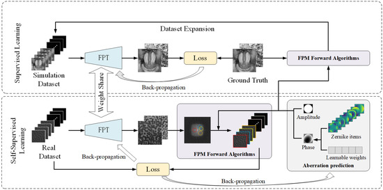
Figure 1.
Semi-supervised FPT training process diagram.
4. Fourier Ptychographic Transformer Backbone Network
We utilized a Fourier ptychographic transformer (FPT) as the backbone network [32], providing an efficient end-to-end training paradigm with rapid inference capabilities. As shown at the top panel in Figure 2, the network utilizes all low-resolution amplitude images as the input to ensure the complete information required for reconstruction. The architecture is primarily composed of convolutional neural networks (CNNs) and a self-attention mechanism [35]. The initial layers of the network employ convolutional operations for feature extraction, where the translation invariance and local receptive field properties of convolution are well suited for capturing shallow texture features of images. The deeper layers employs self-attention mechanism for extracting complex, high-dimensional features [36]. The self-attention mechanism effectively captures long-range dependencies, enabling super-resolution and phase recovery.
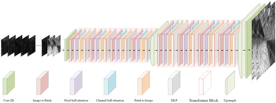
Figure 2.
FPT architecture diagram.
The input of the network consists of 225 channels’ low-resolution amplitude images, denoted as , where H and W represent the height and width of the amplitude image, while C denotes the channel dimension which is 225. Initially, the shallow texture feature extraction is performed through a convolutional layer to obtain . Subsequently, deep feature extraction is carried out using 8 transformer blocks, each comprising an image to patch module, a pixel self-attention module, a channel self-attention module, a patch to image module, and a multi-layer perceptron (MLP) module.
In each transformer block, is first converted into a window patch sequence via the image to patch module, which is inspired by the shifted windows in the Swin transformer [37], where H represents the window patch size. This module alternates pixel assignments into patches, ensuring that the deep network captures long-range spatial dependencies. Then, feature extraction is conducted along two dimensions: the pixel self-attention module calculates the self-attention relationship among pixels within each spatial patch, focusing on capturing spatial-level detail features, expressed as follows:
where represents the reshape of , and represent linear transformations that preserve dimensional consistency. The channel self-attention module computes the self-attention relationships among channel features, thereby enhancing the network capacity to promote cross-channel interactions, expressed as follows:
where represents the reshape of . The results from both attention modules are then summed and restored to image distribution through the patch to image module, yielding , which is subsequently fed into the MLP for nonlinear feature extraction, producing the block output . The upsample module achieves super-resolution enhancement through pixel transformation. Finally, a convolutional layer performs channel fusion, outputting high-resolution amplitude and phase images.
Loss Function
The loss function is composed of three parts: L1 loss, SSIM [38] loss between the output amplitude and phase of the network and the ground truth, as well as the amplitude loss between the reconstructed low-resolution amplitudes and the input amplitudes.
where n denotes the number of pixels in a amplitude, m denotes the number of LEDs, denotes the forward downsampling process of FPM, denotes the mean of , represents the standard deviation of , signifies the covariance of , are constant, and are hyper-parameters. During Stage 1 of self-supervised learning, , while and ; during Stage 2 of supervised learning, , and both and .
5. Experiments
5.1. Training Details
The network was trained on an NVIDIA GTX 4090 for a total of 200 epochs. The batch size used for training was 4, with an initial learning rate of , which was reduced by 25% every 30 epochs. The optimizer employed was Adaptive Moment Estimation (Adam). The entire training process took approximately 2 h.
5.2. Experimental System and Model Parameters
The FPM experimental system we use includes the following parameters: the objective lens NA is 0.16, optical magnification is 4×, the LED array consists of 15 × 15 LEDs spaced 2 mm apart, the illumination wavelength is 0.625 m, the pixel size of the CCD camera is 4.4 m, and the vertical distance between the sample plane and the LED array is 60 mm. The model’s hyperparameters are configured as follows: it employs 8 transformer blocks, an embedding dimension of 512, and a window patch size of 16. The overall computational complexity of the model is 667 GFLOPs, with approximately 31.8 M parameters. The inference time is approximately 100 ms.
5.3. Reconstruction Results
The augmented training dataset used the Div2k [39] dataset, which is rich in high-frequency details as the ground truth. Corresponding low-resolution amplitude sequences were generated using the FPM forward process, with all system parameters consistent with the real experimental setup.
5.3.1. Simulated Dataset Reconstruction
To validate the efficacy of the proposed method, we conducted simulations comparing the two-stage reconstruction performance of the network under varying intensities of noise and optical aberrations. Gaussian-distributed noise with a mean of zero and variances of 0.10, 0.05, and 0.01 was introduced. The comparative results are illustrated in Figure 3. As shown in Figure 3, it is evident that even in the presence of noise effects of different intensities, the first stage of the network effectively reconstructs the pupil function with aberrations, while the supervised learning in the second stage significantly enhances the reconstruction outcomes in terms of SSIM and PSNR.
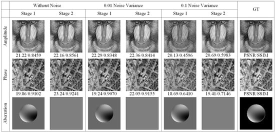
Figure 3.
Visual comparison of SFPT simulation reconstruction results under various noise variances.
Further comparative analysis of simulated dataset reconstructions using various methods is presented in Figure 4, where we conducted comparative experiments between the traditional FPM algorithm, the deep learning-based FuNN [26], and SFPT. As shown in Figure 4, our method attains superior performance in PSNR and SSIM metrics for amplitude and phase reconstruction, exhibiting noticeably reduced visual artifacts.
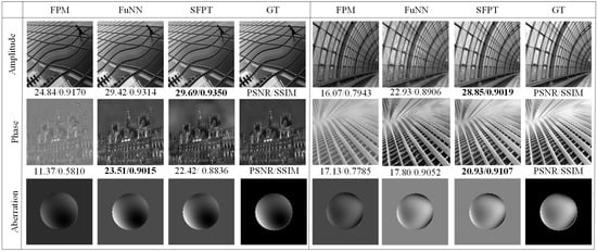
Figure 4.
Visual comparison of different methods’ reconstruction results (the values in bold are the best measurements in each group).
5.3.2. Real Experiment Dataset Reconstruction
To further substantiate the network efficacy in a real experimental environment, we utilized a real experimental system to collect the red blood cell dataset and compared results of different reconstruction methods, as illustrated in Figure 5. As shown in Figure 5, our method produces clearer visual outcomes on real data, while the aberration reconstruction is also comparable to that of traditional FPM pupil aberration reconstruction.
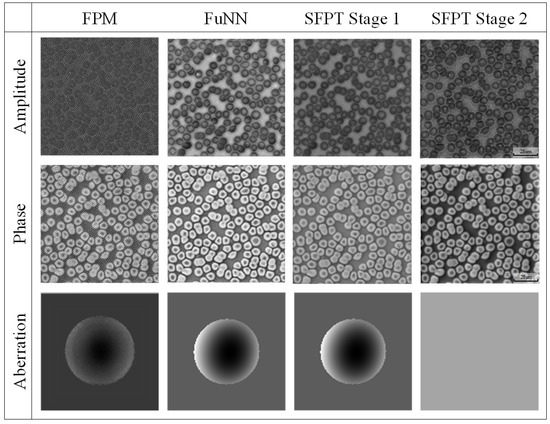
Figure 5.
The visual comparison of the different methods reconstructs results in a real erythrocytes’ dataset.
We further collected a variety of samples such as fibers, human vein cells and plexus. Moreover, we compared their reconstruction results in the two stages of the SFPT, as illustrated in Figure 6. As shown in Figure 6, the supervised learning in the second stage effectively enhances the visual fidelity of the reconstructed amplitude and phase. The clearer phase reconstruction accurately reflects the refractive index distribution of the cells, thereby indirectly revealing cellular metabolic activity, pathological states, and physiological processes such as proliferation or apoptosis.
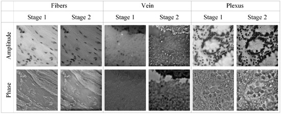
Figure 6.
The visual comparison of the SFPT two-stage reconstruction results in real dataset.
5.4. Phase Unwrapping
To enable the network to learn the mapping from low-resolution amplitude images to high-resolution unwrapped phase image, we set the ground truth phase range for the Stage 2 to −2 to 2 and generate an augmented dataset to train the network. The reconstruction capability of SFPM for thicker samples with phase ranges exceeding 2 was validated using a simulated dataset. The reconstruction results are presented in Figure 7. As shown in Figure 7, SFPM demonstrates a certain degree of reconstruction capability for phase data exceeding 2.
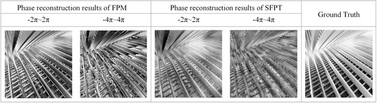
Figure 7.
The visual comparison of the reconstruction results for different phase ranges between FPM and SFPM.
To further validate the model’s performance on in a real experimental environment, we captured images of bullfrog erythrocytes, approximately 16–25 m thick [40], and the phase range was calculated to be approximately 2 to 4 in water. We compared the reconstructed phase of traditional FPM with the reconstructed phase obtained by SFPT trained on different phase range datasets; the reconstruction results are shown in Figure 8:
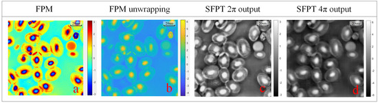
Figure 8.
The visual comparison of the different unwrapping results in bullfrog erythrocytes dataset. (a) FPM reconstruction results. (b) FPM reconstruction unwrapping results. (c) SFPT wrapping reconstruction results. (d) SFPT unwrapping reconstruction results.
Figure 8c shows the inference results of the network trained with an augmented dataset generated using phase values distributed from − to , while Figure 8d shows the inference results of the network trained with an augmented dataset generated using phase values distributed from −2 to 2. Comparing the traditional FPM algorithm and unwrapping algorithms, it is evident that the dataset trained with the − to phase distribution encounters phase saturation problems when reconstructing phases beyond the 2 period.
In contrast, the reconstruction results in Figure 8d exhibit distinct cell nuclei that resemble the unwrapped phase output of the FPM algorithm, indicating that adjusting the distribution of training data enables the network to accurately reconstruct the authentic phase. This method allows the network to precisely restore the unwrapped phase without incurring additional costs.
5.5. Ablation Experiment
To validate the necessity of each key module in SFPT, we performed ablation experiments, with the results presented in Table 1. As shown in Table 1, supervised learning, Zernike modes, and the pixel and channel self-attention mechanism in the transformer network all contribute to varying degrees of improvement in the reconstruction results.

Table 1.
Results of the SFPT key module ablation experiment.
6. Conclusions
In this paper, we introduce a semi-supervised Fourier ptychographic microscopy reconstruction network based on the FPT, termed SFPT. SFPT harnesses the sequence modeling capabilities of the FP-transformer to effectively reconstruct high-resolution amplitude and phase, integrates the FPM forward algorithm with Zernike modes for aberration correction and utilizes augmented datasets to learn the unwrapping phase.
Through comparative reconstruction results on simulated and real data, we demonstrate that our method can efficaciously perform a super-resolution reconstruction of amplitude and phase even in the presence of aberrations and noise interference. By adjusting the distribution domain of a network’s training dataset, we achieved phase unwrapping within a specified range and conducted comparative validation on real data, underscoring the effectiveness of the proposed method. However, the proposed method still has several limitations. For instance, SFPT demands substantial computational resources, with the computational cost of the transformer escalating rapidly as the image size increases. For larger images, it requires partitioning the image for reconstruction and subsequent stitching. Additionally, the method necessitates at least 12GB of GPU memory for model training. Although the network demonstrates a certain degree of robustness, it needs to be fine-tuned when dealing with significant variations in aberrations, which incurs additional time costs. In future works, we will explore more lightweight reconstruction algorithms and effective strategies for real-time dynamic FPM reconstructions, which represents the mainstream trajectory for advancing the practical applicability of FPM.
Author Contributions
Conceptualization, X.Z., H.T., E.O., L.Z. and H.F.; methodology, X.Z.; software, X.Z.; validation, X.Z., H.T. and H.F.; formal analysis, X.Z.; investigation, X.Z.; resources, H.F.; data curation, X.Z.; writing—original draft preparation, X.Z.; writing—review and editing, X.Z. and E.O.; visualization, X.Z.; supervision, L.Z. and H.F.; project administration, H.F.; funding acquisition, H.F. All authors have read and agreed to the published version of the manuscript.
Funding
This research was funded by the National Natural Science Foundation of China (12074268), the Shenzhen Science and Technology Major Project (KJZD20230923114601004) and the Scientific Instrument Developing Project of Shenzhen University (2023YQ024).
Institutional Review Board Statement
Not applicable.
Informed Consent Statement
Not applicable.
Data Availability Statement
The code of this study will be publicly accessible in a GitHub repository at https://github.com/pilixiaohui/SFPT (accessed on 27 December 2024).
Conflicts of Interest
The authors declare no conflicts of interest. The funders had no role in the design of the study, in the collection, analyses, or interpretation of data, in the writing of the manuscript, or in the decision to publish the results.
References
- Zheng, G.; Horstmeyer, R.; Yang, C. Wide-field, high-resolution Fourier ptychographic microscopy. Nat. Photonics 2013, 7, 739–745. [Google Scholar] [CrossRef] [PubMed]
- Zheng, G.; Shen, C.; Jiang, S.; Song, P.; Yang, C. Concept, implementations and applications of Fourier ptychography. Nat. Rev. Phys. 2021, 3, 207–223. [Google Scholar] [CrossRef]
- Ou, X.; Horstmeyer, R.; Yang, C.; Zheng, G. Quantitative phase imaging via Fourier ptychographic microscopy. Opt. Lett. 2013, 38, 4845–4848. [Google Scholar] [CrossRef] [PubMed]
- Pan, A.; Zuo, C.; Yao, B. High-resolution and large field-of-view Fourier ptychographic microscopy and its applications in biomedicine. Rep. Prog. Phys. 2020, 83, 096101. [Google Scholar] [CrossRef]
- Xu, F.; Wu, Z.; Tan, C.; Liao, Y.; Wang, Z.; Chen, K.; Pan, A. Fourier Ptychographic Microscopy 10 Years on: A Review. Cells 2024, 13, 324. [Google Scholar] [CrossRef]
- Tian, L.; Liu, Z.; Yeh, L.H.; Chen, M.; Zhong, J.; Waller, L. Computational illumination for high-speed in vitro Fourier ptychographic microscopy. Optica 2015, 2, 904–911. [Google Scholar] [CrossRef]
- Zhang, Y.; Jiang, W.; Tian, L.; Waller, L.; Dai, Q. Self-learning based Fourier ptychographic microscopy. Opt. Express 2015, 23, 18471–18486. [Google Scholar] [CrossRef]
- Sun, J.; Zuo, C.; Zhang, L.; Chen, Q. Resolution-enhanced Fourier ptychographic microscopy based on high-numerical-aperture illuminations. Sci. Rep. 2017, 7, 1187. [Google Scholar] [CrossRef]
- Sun, J.; Zuo, C.; Zhang, J.; Fan, Y.; Chen, Q. High-speed Fourier ptychographic microscopy based on programmable annular illuminations. Sci. Rep. 2018, 8, 7669. [Google Scholar] [CrossRef]
- Bian, L.; Suo, J.; Zheng, G.; Guo, K.; Chen, F.; Dai, Q. Fourier ptychographic reconstruction using Wirtinger flow optimization. Opt. Express 2015, 23, 4856–4866. [Google Scholar] [CrossRef]
- Pan, A.; Zhang, Y.; Zhao, T.; Wang, Z.; Dan, D.; Lei, M.; Yao, B. System calibration method for Fourier ptychographic microscopy. J. Biomed. Opt. 2017, 22, 096005. [Google Scholar] [CrossRef] [PubMed]
- Nguyen, T.; Xue, Y.; Li, Y.; Tian, L.; Nehmetallah, G. Deep learning approach for Fourier ptychography microscopy. Opt. Express 2018, 26, 26470–26484. [Google Scholar] [CrossRef] [PubMed]
- Konda, P.C.; Loetgering, L.; Zhou, K.C.; Xu, S.; Harvey, A.R.; Horstmeyer, R. Fourier ptychography: Current applications and future promises. Opt. Express 2020, 28, 9603–9630. [Google Scholar] [CrossRef] [PubMed]
- Bouchama, L.; Dorizzi, B.; Thellier, M.; Klossa, J.; Gottesman, Y. Fourier ptychographic microscopy image enhancement with bi-modal deep learning. Biomed. Opt. Express 2023, 14, 3172–3189. [Google Scholar] [CrossRef]
- Wang, X.; Piao, Y.; Jin, Y.; Li, J.; Lin, Z.; Cui, J.; Xu, T. Fourier Ptychographic Reconstruction Method of Self-Training Physical Model. Appl. Sci. 2023, 13, 3590. [Google Scholar] [CrossRef]
- Wang, Y.; Guan, N.; Li, J.; Wang, X. A Virtual Staining Method Based on Self-Supervised GAN for Fourier Ptychographic Microscopy Colorful Imaging. Appl. Sci. 2024, 14, 1662. [Google Scholar] [CrossRef]
- Lu, X.; Wang, M.; Wu, H.; Hui, F. Deep learning for fast image reconstruction of Fourier ptychographic microscopy with expanded frequency spectrum. In Proceedings of the 4th Optics Young Scientist Summit (OYSS 2020), Ningbo, China, 4–7 December 2020; SPIE: Pune, India, 2021; Volume 11781, pp. 146–152. [Google Scholar]
- Kappeler, A.; Ghosh, S.; Holloway, J.; Cossairt, O.; Katsaggelos, A. Ptychnet: CNN based Fourier ptychography. In Proceedings of the 2017 IEEE International Conference on Image Processing (ICIP), Beijing, China, 17–20 September 2017; IEEE: Piscataway, NJ, USA, 2017; pp. 1712–1716. [Google Scholar]
- Zhang, J.; Xu, T.; Shen, Z.; Qiao, Y.; Zhang, Y. Fourier ptychographic microscopy reconstruction with multiscale deep residual network. Opt. Express 2019, 27, 8612–8625. [Google Scholar] [CrossRef]
- Bardozzo, F.; Fiore, P.; Valentino, M.; Bianco, V.; Memmolo, P.; Miccio, L.; Brancato, V.; Smaldone, G.; Gambacorta, M.; Salvatore, M.; et al. Enhanced tissue slide imaging in the complex domain via cross-explainable GAN for Fourier ptychographic microscopy. Comput. Biol. Med. 2024, 179, 108861. [Google Scholar] [CrossRef]
- Feng, T.; Wang, A.; Wang, Z.; Liao, Y.; Pan, A. Linear-space-variant model for Fourier ptychographic microscopy. Opt. Lett. 2024, 49, 2617–2620. [Google Scholar] [CrossRef]
- Wu, K.; Pan, A.; Sun, Z.; Shi, Y.; Gao, W. Blind deep-learning based preprocessing method for Fourier ptychographic microscopy. Opt. Laser Technol. 2024, 169, 110140. [Google Scholar] [CrossRef]
- Chen, Q.; Huang, D.; Chen, R. Fourier ptychographic microscopy with untrained deep neural network priors. Opt. Express 2022, 30, 39597–39612. [Google Scholar] [CrossRef] [PubMed]
- Jiang, S.; Guo, K.; Liao, J.; Zheng, G. Solving Fourier ptychographic imaging problems via neural network modeling and TensorFlow. Biomed. Opt. Express 2018, 9, 3306–3319. [Google Scholar] [CrossRef] [PubMed]
- Zhang, J.; Xu, T.; Li, J.; Zhang, Y.; Jiang, S.; Chen, Y.; Zhang, J. Physics-based learning with channel attention for Fourier ptychographic microscopy. J. Biophotonics 2022, 15, e202100296. [Google Scholar] [CrossRef] [PubMed]
- Zhang, J.; Tao, X.; Yang, L.; Wang, C.; Tao, C.; Hu, J.; Wu, R.; Zheng, Z. The integration of neural network and physical reconstruction model for Fourier ptychographic microscopy. Opt. Commun. 2022, 504, 127470. [Google Scholar] [CrossRef]
- Wang, Y.; Wang, Y.; Li, J.; Wang, X. Fourier Ptychographic Microscopy Reconstruction Method Based on Residual Local Mixture Network. Sensors 2024, 24, 4099. [Google Scholar] [CrossRef]
- Wu, K.; Pan, A.; Gao, W. Fourier ptychographic reconstruction with denoising diffusion probabilistic models. Opt. Laser Technol. 2024, 176, 111016. [Google Scholar] [CrossRef]
- Herráez, M.A.; Burton, D.R.; Lalor, M.J.; Gdeisat, M.A. Fast two-dimensional phase-unwrapping algorithm based on sorting by reliability following a noncontinuous path. Appl. Opt. 2002, 41, 7437–7444. [Google Scholar] [CrossRef]
- Ghiglia, D.C.; Romero, L.A. Robust two-dimensional weighted and unweighted phase unwrapping that uses fast transforms and iterative methods. JOSA A 1994, 11, 107–117. [Google Scholar] [CrossRef]
- Wang, L.; Liang, W.; Guo, W.; Wang, Z.; Wang, C.; Gao, Q. Multi task deep learning phase unwrapping method based on semantic segmentation. J. Opt. 2024, 26, 115709. [Google Scholar] [CrossRef]
- Zhao, L.; Zhou, X.; Lu, X.; Tong, H.; Fang, H. Transformer-based reconstruction for Fourier ptychographic microscopy. IEEE Access 2023, 11, 94536–94544. [Google Scholar] [CrossRef]
- Zhu, X.J. Semi-Aupervised Learning Literature Survey. University of Wisconsin-Madison. 2008. Available online: https://pages.cs.wisc.edu/~jerryzhu/pub/ssl_survey.pdf (accessed on 9 December 2024).
- Ou, X.; Zheng, G.; Yang, C. Embedded pupil function recovery for Fourier ptychographic microscopy. Opt. Express 2014, 22, 4960–4972. [Google Scholar] [CrossRef] [PubMed]
- Vaswani, A.; Shazeer, N.; Parmar, N.; Uszkoreit, J.; Jones, L.; Gomez, A.N.; Kaiser, Ł.; Polosukhin, I. Attention is all you need. In Proceedings of the 31st International Conference on Neural Information Processing Systems, Long Beach, CA, USA, 4–9 December 2017; pp. 6000–6010. [Google Scholar]
- Ouyang, E.; Li, B.; Hu, W.; Zhang, G.; Zhao, L.; Wu, J. When Multigranularity Meets Spatial–Spectral Attention: A Hybrid Transformer for Hyperspectral Image Classification. IEEE Trans. Geosci. Remote. Sens. 2023, 61, 1–18. [Google Scholar] [CrossRef]
- Liu, Z.; Lin, Y.; Cao, Y.; Hu, H.; Wei, Y.; Zhang, Z.; Lin, S.; Guo, B. Swin transformer: Hierarchical vision transformer using shifted windows. In Proceedings of the IEEE/CVF International Conference on Computer Vision, Virtual Conference, 10 March 2021; pp. 10012–10022. [Google Scholar]
- Wang, Z.; Bovik, A.C.; Sheikh, H.R.; Simoncelli, E.P. Image quality assessment: From error visibility to structural similarity. IEEE Trans. Image Process. 2004, 13, 600–612. [Google Scholar] [CrossRef] [PubMed]
- Agustsson, E.; Timofte, R. Ntire 2017 challenge on single image super-resolution: Dataset and study. In Proceedings of the 2017 IEEE Conference on Computer Vision and Pattern Recognition Workshops (CVPRW), Honolulu, HI, USA, 21–26 July 2017; pp. 126–135. [Google Scholar]
- Coppo, J.A.; Mussart, N.B.; Fioranelli, S.A. Blood and urine physiological values in farm-cultured Rana catesbeiana (Anura: Ranidae) in Argentina. Rev. Biol. Trop. 2005, 53, 545–559. [Google Scholar] [CrossRef] [PubMed]
Disclaimer/Publisher’s Note: The statements, opinions and data contained in all publications are solely those of the individual author(s) and contributor(s) and not of MDPI and/or the editor(s). MDPI and/or the editor(s) disclaim responsibility for any injury to people or property resulting from any ideas, methods, instructions or products referred to in the content. |
© 2025 by the authors. Licensee MDPI, Basel, Switzerland. This article is an open access article distributed under the terms and conditions of the Creative Commons Attribution (CC BY) license (https://creativecommons.org/licenses/by/4.0/).