Identifying the Initial Corrosion Fatigue Failure Based on Dropping Electrochemical Potential

Abstract

The corrosion fatigue of duplex stainless-steel X2CrNiMoN22-5-3 can be determined by purely alternating axial cyclic load to failure using hour-glass shaped specimens. The experimental setup comprises a corrosion chamber allowing for the circulation of an aquifer electrolyte heated to 369 K simulating a carbon capture and storage as well as geothermal power plant environment. During engineering of a carbon storage site or geothermal power plant, it may be crucial to determine the failure onset of a component beforehand. Therefore, an algorithm with 93.3% reliability was established based on splitting the measured potential values into ten time series with a capacity of ten values. The failure of corrosion fatigue specimens in a geothermal environment correlates to the drop of the curves of the electrochemical potential which is measured simultaneously within the corrosion chamber. Crack initiation was, therefore, successfully derived from the electrochemical potential.

1. Introduction

In the context of carbon capture and storage (CCS) and future geothermal energy extraction applications, such as those involving injection pipes, delivery pumps, and filtration components, engineering materials face new challenges. These materials must be able to withstand both mechanical stress and exposure to highly corrosive environments. Mechanical stress, especially cyclic loading, combined with factors like temperature and chloride concentration, has a significant impact on corrosion processes [1]. In high-alloy steels, corrosion fatigue becomes more severe in the presence of low chromium content [2], chlorides [3], hydrogen sulfide (H₂S) [4], and carbon dioxide (CO₂) [5]. Increased temperature, mechanical loading, and lower pH levels further reduce the endurance limit, worsening corrosion fatigue (CF) in these steels [6].

Studies show a strong connection between the mechanical and corrosion properties of different steel types and their surface conditions resulting from machining processes [7,8,9,10,11]. In general, reducing surface depth enhances corrosion resistance in carbon steel [8], austenitic stainless steel after shot peening [11], and ferritic stainless steel when the surface roughness R_a exceeds 0.5 µm [10]. Notably, internal pipeline corrosion is more influenced by relative humidity than by initial surface roughness, with lowering humidity being more effective than altering the surface condition [9]. Additionally, smoother surfaces and internal compressive surface stresses are linked to better fatigue performance in air, even in corrosive environments. This correlation extends to improved corrosion resistance, which in turn improves endurance limits and enhances corrosion fatigue behavior [12,13,14,15].

1.1. Corrosion Fatigue of Standard Duplex Stainless-Steel X2CrNiMoN22-5-3

Duplex stainless-steel (DSS) X2CrNiMoN22-5-3 (AISI 2205) with a ferritic–austenitic microstructure, often used in industries such as chemical processing, refineries, and desalination plants [16], is known for its high mechanical strength [16], durability in corrosive conditions [17], and resistance to stress corrosion cracking [18].

The following general findings refer to earlier experiments summarized by Pfennig et al. [19] and Wolf [20] and characterize the corrosion fatigue CF behavior of X2CrNiMoN22-5-3 used within this study. Later, necessary results will be mentioned as they are needed to follow the experimental procedure and theoretical evaluation.

In non-corrosive environments, the fatigue limit of DSS X2CrNiMoN22-5-3 is around 485 MPa (Pf = 50%, push/pull) after 10⁷ cycles. However, when exposed to CCS or corrosive geothermal environments such as the geothermal brine from the Northern German Basin at 98 °C, and tested under stress between 175 and 325 MPa, the material lasted for up to 9.2 million cycles at a stress amplitude of 240 MPa and free corrosion potential. The maximum number of cycles was 4.2 × 10⁶ at a stress amplitude of 290 MPa without isolation of the specimen against the test machine and 9.2 × 10⁶ cycles at 160 MPa with insulation. Cracks followed a curved path mainly degrading the austenitic phase. Fatigue strength is significantly reduced due to local corrosion (pitting) from carbonic acid, rather than mechanical loading, as the primary cause of crack initiation and intercrystalline crack propagation.

Surface roughness plays a key role in mechanical and corrosion properties, with smoother surfaces, deeper plastic deformations, and compressive surface stresses contributing to a lower endurance limit [14]. Polished surfaces improve fatigue life at low stresses, while technical finishes are more effective at high stresses, where microcracks dominate failure. For polished and technical surfaces, the corrosion rates were below 0.005 mm/year, while rates increased to 0.035 mm/year after shot peening. In a geothermal and CCS environment, the main phases precipitating on the surface, regardless of surface roughness, were carbonates or hydroxides such as FeCO₃ and FeOOH. Technical surfaces endured a higher number of cycles before failure (P50% at S_a 300 MPa = 5 × 10⁵, k = 19.006) at stress levels above 275 MPa, compared to polished surfaces (P50% at S_a 300 MPa = 1.5 × 10⁵, k = 8.78).

The failure mechanism of X2CrNiMoN22-5-3 appears to be similar across surface conditions, given the relatively narrow scatter ranges (TN = 1:1.35 for technical surfaces and TN = 1:1.95 for polished surfaces). Early formation of pits and localized depassivation likely play a role in crack initiation, as they are linked to early mechanical degradation. Earlier, the authors showed that a consistent drop in potential (both in absolute value and angle of inclination) at the free corrosion potential [21] signals the start of failure in standard duplex stainless-steel X2CrNiMoN22-5-3. Just before crack initiation, the drop in potential aligns with the increasing fatigue crack area and matches the predicted growth in crack propagation speed [20,21].

1.2. Aim and Interest of This Study

Up to now there are no data available upon the correlation of frequency, electrochemical behavior, and initial failure during corrosion fatigue to predict early failure from monitoring the combined data within the system. Therefore, this study investigates the relationship between crack initiation and failure during corrosion fatigue experiments, focusing on the correlation between the onset of failure (appointed by a drop in frequency) and changes in electrochemical potential. By examining how these factors are linked, this research aims to identify crack initiation as a significant cause of failure. The findings highlight the critical role that electrochemical potential shifts and frequency variations play in the early stages of crack development, offering valuable insights into the mechanisms behind material degradation and the estimation of failure.

The importance of the findings lies in the development and successful implementation of an algorithm that predicts early failure during corrosion fatigue in duplex stainless-steel specimens exposed to a highly corrosive geothermal environment. By leveraging real-time electrochemical potential measurements from a custom test setup [19,20], the algorithm demonstrates a strong correlation between potential curve behavior and failure onset, achieving a predictive accuracy of 93%. This innovative approach combines tailored data analysis techniques, such as splitting time series and applying regression, to establish a practical, efficient tool for anticipating material failure in highly corrosive and mechanically stressed conditions, offering significant implications for geothermal energy and CCS industries.

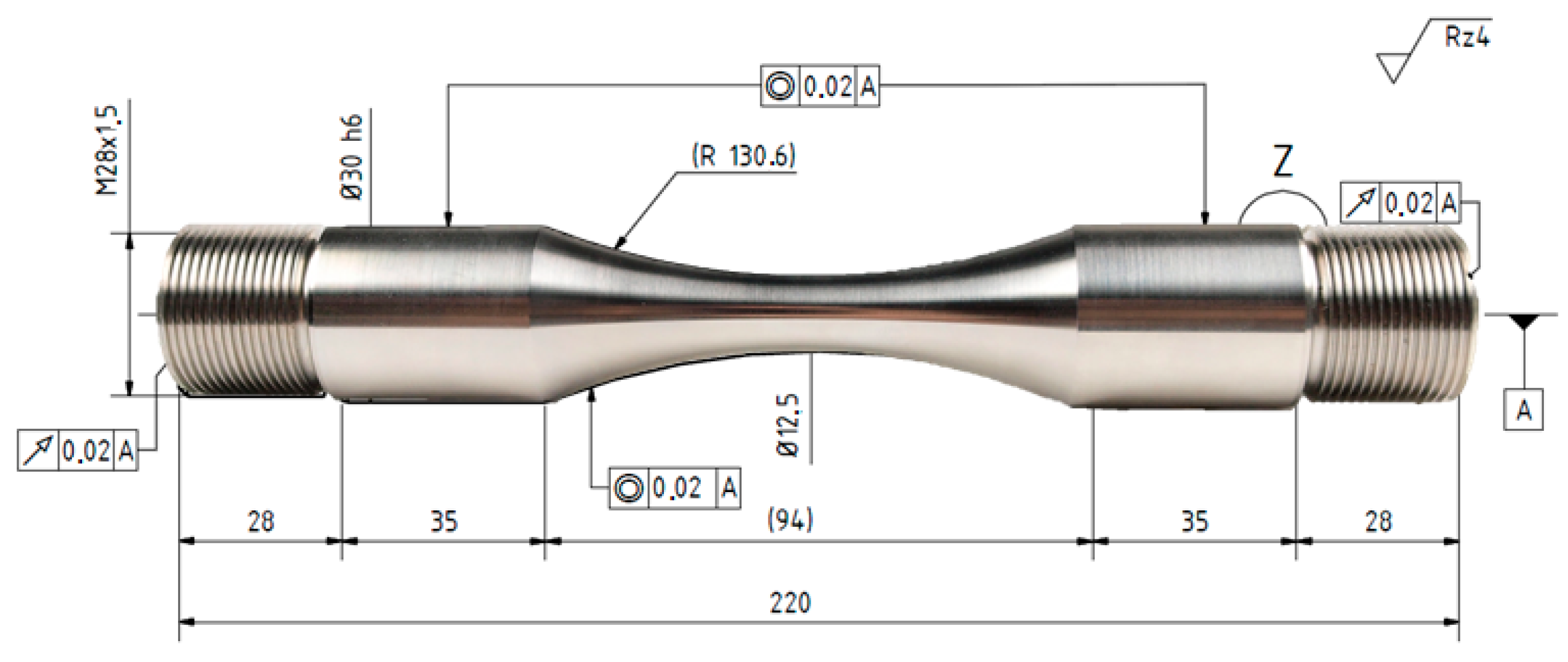
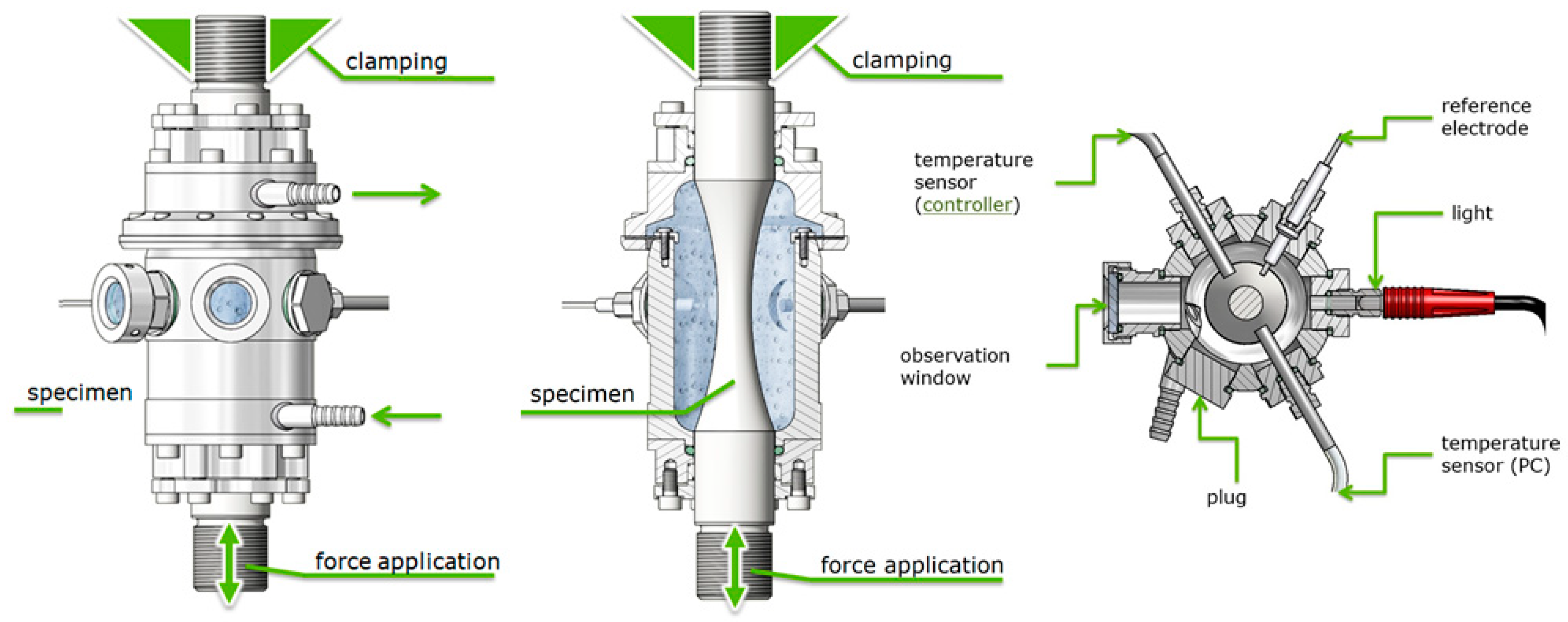
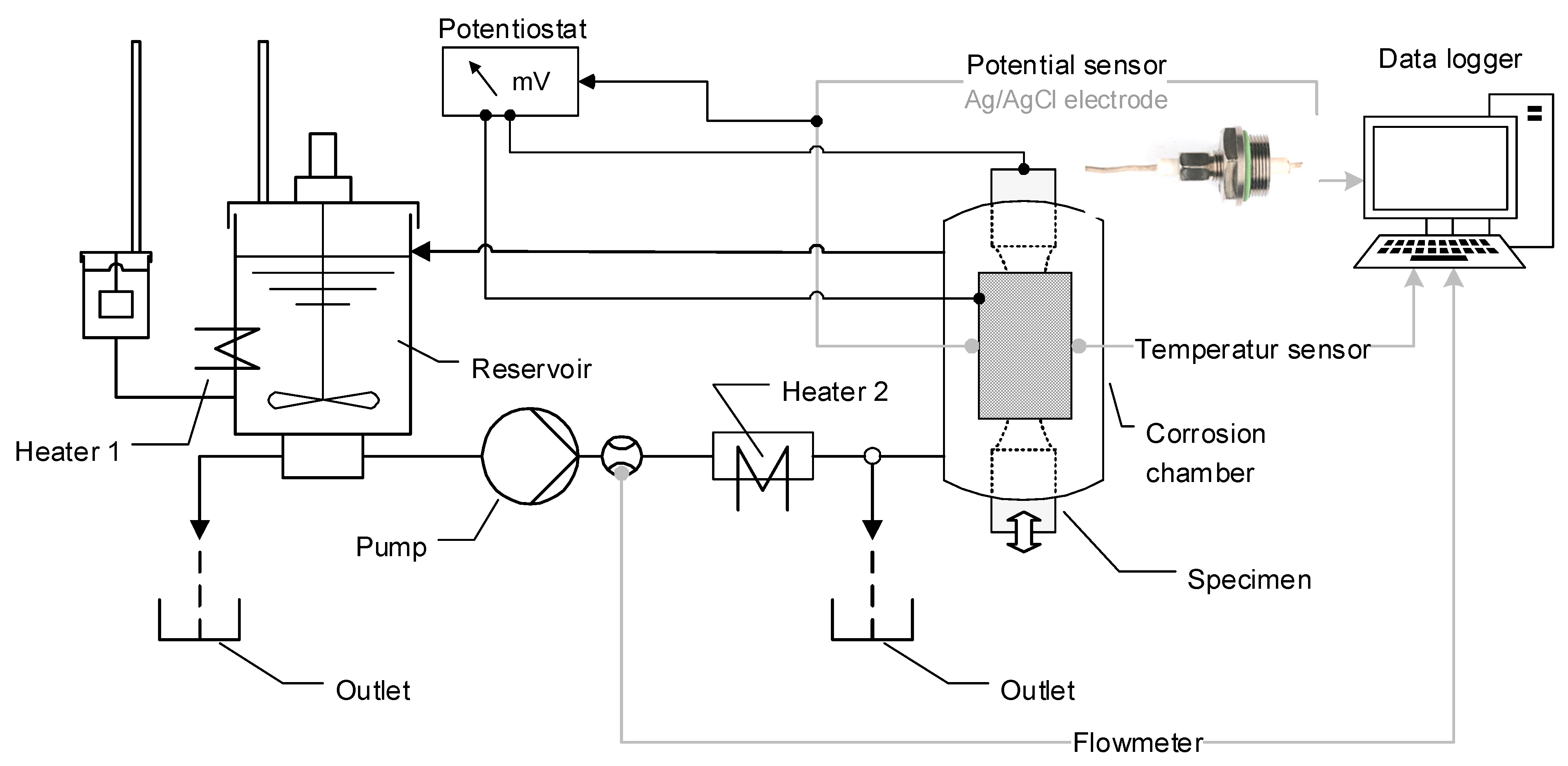
2. Materials and Methods

Material: corrosion fatigue testing was conducted on standard duplex stainless-steel X2CrNiMoN22-5-3, 1.4462 (yield strength: 672 MPa, tensile strength: 854 MPa, and PREN number referring to corrosion resistance: 35.1 [19,20]). The steel was continuously casted, tempered appropriately, and quenched in water resulting in a phase equilibrium of ferrite and austenite (

Table 1. X2CrNiMoN 22 5 3 (EN/DIN 1.4462, UNS S31803); chemical composition in mass percent.

Phases	C	Si	Mn	Cr	Mo	Ni	N
α & γ **	0.023	0.48	1.83	22.53	2.92	5.64	0.15
α *	0.02	0.55	1.59	24.31	3.62	3.81	0.07
γ *	0.03	0.47	1.99	20.69	2.17	6.54	0.28

* PREN α = 37.4; γ = 32.4; ** p = 0.024; S = 0.008.

). Analysis via spark emission spectrometry (SPEKTROLAB M, SPECTRO Analytical Instruments GmbH, Kleve, Germany) and the Electron Probe Microanalyzer JXA8900-RLn, JEOL Ltd., Tokyo, Japan, (Table 1) offered the precise chemical composition. The high pitting resistance number PREN of standard duplex stainless-steel X2CrNiMoN22-5-3 represents sufficient corrosion resistance based on the critical chemical composition of >12% chromium and a moderate percentage of nickel and sufficient nitrogen and manganese content. Especially, the high chromium content guarantees good corrosion resistance against both surface and local corrosive attack in aggressive geothermal environments.

Samples: round corrosion fatigue samples of X2CrNiMoN22-5-3, featuring shoulder heads, were produced through precision turning (Rz = 4), in accordance with DIN EN ISO 11782-1 [22] and the FKM Research Issue 217 guidelines (Figure 1). The same dimensions of the test specimen have been used in previous corrosion fatigue tests to characterize the endurance limit and corrosion fatigue behavior of X2CrNiMoN22-5-3 [6,19,20,21]. The critical region of the specimen, exposed to the corrosive medium, was polished by first grinding with SiC paper ranging from 180 grit to 1200 grit under water, followed by a final polishing using diamond paste in 6 µm, 3 µm, and 1 µm grades. The surface roughness of the polished samples ranged from 0.58 µm to 2.01 µm, with an average of 1.59 µm.

Artificial geothermal brine (corrosion media): in order to replicate the actual geothermal conditions, geothermal aquifer water—comparable to that of the Stuttgart Aquifer [23] and the Northern German Basin (NGB) [24,25]—was carefully synthesized. The process followed a precise sequence to prevent the formation of salts and carbonates, as outlined in

Table 2. Synthetic aquifer water according to the chemical composition of the Northern German Basin (NGB) and Stuttgart Formation electrolyte or according to the Stuttgart Formation.

According to the Northern German Basin or According to Stuttgart Formation
	NaCl	KCl	CaCl2 × 2H2O	MgCl2 × 6H2O	NH4Cl	ZnCl2	SrCl2 × 6H2O	PbCl2	Na2SO4	Ph Value
g/L	98.22	5.93	207.24	4.18	0.59	0.33	4.72	0.30	0.07	5.4–6
	NaCl	KCl	CaCl2 × 2H2O	MgCl2 × 6H2O	Na2SO4 × 10H2O		KOH	NaHCO3
g/L	224.6	0.39	6.45	10.62	12.07		0.321	0.048
	Ca+	K2+	Mg2+	Na2+	Cl−		SO42−	HCO3−		pH value
g/L	1.76	0.43	1.27	90.1	14.33		3.6	0.04		8.2–9

.

Test setup and corrosion fatigue testing: the experimental procedure to determine corrosion fatigue has been described earlier in detail [19,20]: corrosion fatigue testing was carried out on a Schenck-Erlinger Puls PPV machine, operating at a frequency of 33 Hz, with geothermal brine continuously circulating around the specimen. To eliminate any interaction between the specimen and the testing machine, the corrosion chamber was directly attached to the test specimen [19]. Figure 2 represents schematic drawings of the corrosion chamber from the outside (left) and at operation (middle) as well as potential plugs designed for observation, temperature control, lighting, and electrochemical as well as oxygen partial pressure measurements.

The temperature of the corrosion medium, set at 369 K, is controlled by thermal sensors located in both the reservoir and the corrosion chamber. The corrosion medium is circulated from the reservoir to the pump, through the corrosion chamber and back, by a custom-designed, electromagnetically powered gear pump (Figure 2 and Figure 3). Figure 3 gives an overview upon the complete test stand indicating the mechanical tests unit, the heating system, the corrosion chamber, the potentiostat for electrochemical measurements, and the reservoir for corrosive media. The system operates with an actual flow rate of V* = 2.5 × 10⁻⁶ m³/s and a theoretical flow velocity of ω₀ = 1.7 × 10⁻³ m/s at the specimen’s critical section. To simulate CCS conditions, technical CO₂ is fed into the closed system at a rate of approximately 9 L/h [19,20]. The test series involved ten specimens with an insulated test setup, tested under stress levels ranging from 150 to 500 MPa. Given the relatively heterogeneous fine-machined surfaces (surface roughness Rz = 4), the specimens are comparable to prefabricated components.

Electrochemical measurement: electrochemical data are collected during the mechanical tests as well as temperature, pH, and electrochemical potential. A constant potential is maintained via a titanium/titanium-mixed oxide electrode, isolated from both the specimen and the chamber [6,21]. Meanwhile, a shock-resistant Ag/AgCl electrode, positioned within a Teflon channel, acts as a reference to measure the free corrosion potential [6,21] which is evaluated in Section 3.1.

3. Results and Discussion

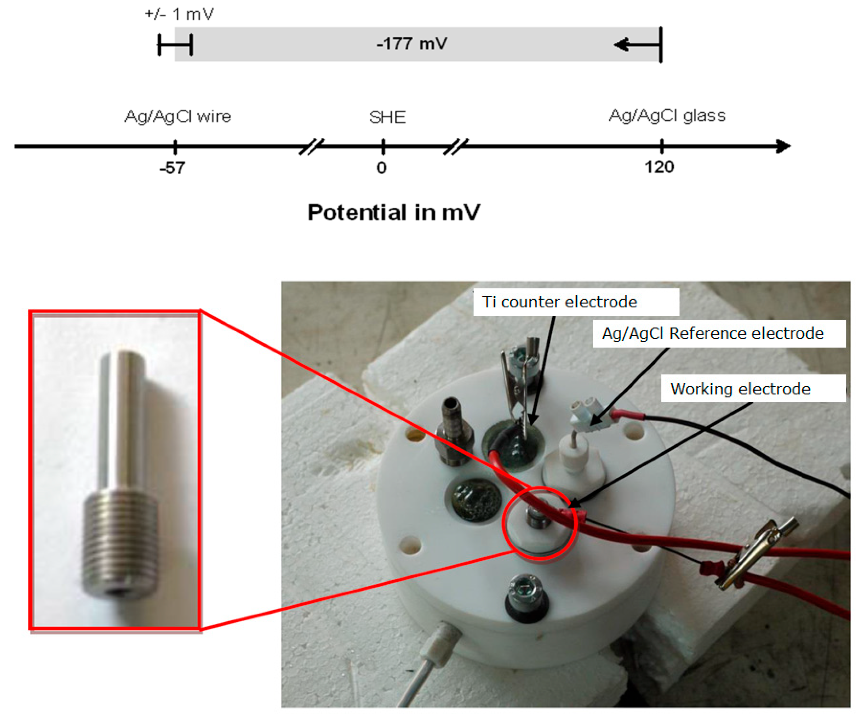
3.1. Evaluation of the Electrode

In the electrochemical experiments, a titanium/titanium-mixed oxide electrode was used to maintain a constant potential within the corrosion chamber, without making electrical contact with the specimen or chamber. A custom-built Ag/AgCl electrode served as the reference, designed for direct measurements near the specimen. This self-manufactured Ag/AgCl electrode, modeled after a standard version, offered increased durability and shock resistance, making it particularly effective for use under cyclic loads. Its design also allowed for reliable operation under high temperatures and severe vibrations, making it well suited for demanding conditions.

To evaluate this Ag/AgCl wire electrode, the electric potential was compared to the potential of a standardized Ag/AgCl glass electrode under experimental boundary conditions. The standardized glass electrode is well known for its design simplicity, repeatability, and stable electric potential that allow trustworthy evaluation of the unknown electrodes and has been introduced in detail earlier [6,26]. The electric potential values obtained were then aligned to the potential value of the standard hydrogen electrode (SHE) for conformity reasons. Applying the standard deviation to values measured, the electric potential of the Ag/AgCl wire electrode was calculated as follows: U_SHE = 120–177 mV = −57 (±1.1 mV). The electric potential of the standardized glass Ag/AgCl electrode at elevated temperatures was obtained from [27]. The graphic representation of the calculation is shown in Figure 4 demonstrating the electric potential of the Ag/AgCl wire electrode in relation to the SHE; the value of the Ag/AgCl glass electrode was adopted from [27]. The setup is shown below.

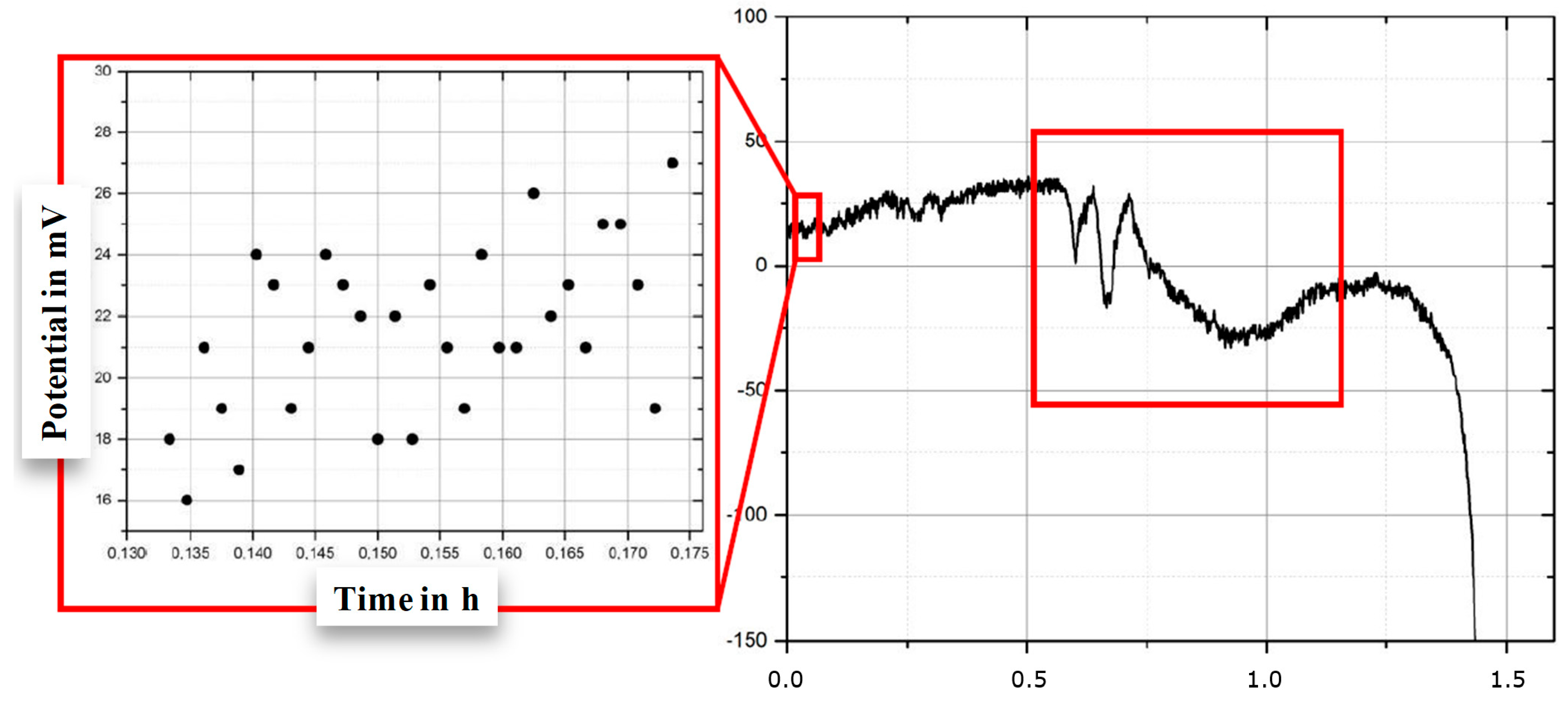
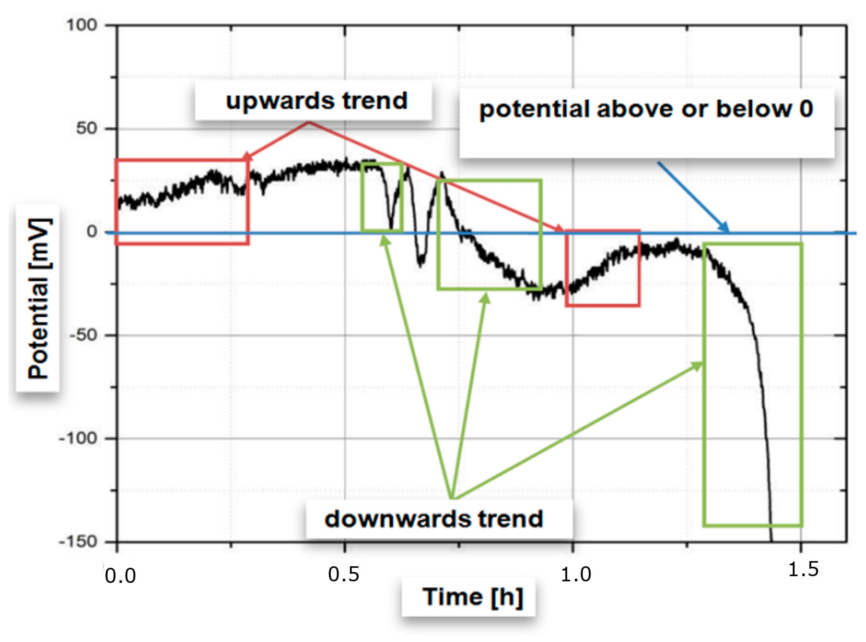
3.2. Relating the Electrical Potential to Fatigue Failure

To correlate early failure of corrosion fatigue specimens in a CCS environment with the drop of the curves determined via in situ measurement of the electrochemical potential (measured directly within the corrosion chamber using the Ag/AgCl wire electrode) 10 free corrosion potentials were analyzed with an insulated experimental test setup (Figure 5). The samples were kept in a reference test stand for 72 h, matching the duration of fatigue testing for 10⁷ cycles in the corrosion chamber. Figure 5 represents four potential pathways of different X2CrNiMoN22-5-3 specimens measured with the Ag/AgCl wire electrode in an insulated fatigue testing setup. It shows the drop in potential over time, highlighting the correlation with the onset of crack propagation in the material. Generally, the measured potential was the same as the initial potential in the chamber, confirming that the test setup did not affect electrochemical measurements. The potential remained largely stable, with significant drops observed during crack formation, leading to specimen failure. This indicates that both mechanical load and crack propagation are key factors influencing potential changes during fatigue testing.

In general, the sudden decrease in electrochemical potential before failure reflects the combined effects of rapid crack propagation, localized anodic activity, and electrochemical instability in the material as it approaches its critical failure point. Crack initiation is accompanied by decreasing frequencies in corrosion fatigue tests. These lower test frequencies enhance crack tip exposure to the corrosive environment, amplifying the potential drop before failure. Rapid crack growth near failure increases the reactive (newly) exposed surface area, intensifying electrochemical activity. In addition, high stress and strain at crack tips create localized anodic regions, accelerating corrosion and affecting potential. Shortly before failure, breakdown of passive films and increased crack interactions lead to a sudden shift in electrochemical potential. The Ag/AgCl electrode detects these changes, reflecting the loss of surface protective properties and increased anodic activity.

Frequency dependence:

Figure 5. Representative samples of potential pathways of different X2CrNiMoN22-5-3 specimens measured with the Ag/AgCl wire electrode in an insulated fatigue testing setup.

Figure 5. Representative samples of potential pathways of different X2CrNiMoN22-5-3 specimens measured with the Ag/AgCl wire electrode in an insulated fatigue testing setup.

In corrosion fatigue experiments, the electrochemical potential decreases with changes in frequency because the rate of mechanical loading influences the interaction between mechanical and electrochemical processes. At lower frequencies, the metal surface is exposed to the corrosive environment for longer periods during each cycle, enhancing electrochemical reactions, such as oxidation and hydrogen evolution, and allowing for more extensive localized electrochemical activity, such as spallation, the accumulation of corrosion products or enhanced anodic dissolution at crack tips. This increases localized anodic dissolution and shifts the potential toward more negative (corrosive) values. Decreasing frequency as means of failure onset therefore always results in decreasing electrochemical potential.

For all corrosion fatigue specimens of standard duplex stainless-steel X2CrNiMoN22-5-3, a potential drop at the free corrosion potential (Figure 5) consistently indicates the onset of failure, both in terms of potential value and angle of decline. Therefore, a sudden drop in potential, along with a frequency change, signals crack initiation. Over the course of the tests, the potential fluctuated by approximately 60 mV (Figure 5). For specimens that did not fail, these potential changes were minimal. Since no clear relationship between surface condition, crack path, or microstructure in the crack region was found, residual stress is the most likely explanation for the final failure [14]. Precision-turned specimens typically had potentials about 50 mV higher than polished specimens [19] (indicating less susceptibility to corrosion processes), because at sufficient high stress amplitudes the lifespan of precision-turned surfaces improves with higher stress amplitudes and short test durations. Note that at long test durations and low stress amplitudes, polished surfaces minimize stress concentration near micro-notch bases, reducing crack initiation and delaying early failures. (As detailed in prior studies summarized in [19], polished surfaces with an Rz of approximately 1.4–1.59 μm exhibit better resistance to degradation than turned surfaces with an Rz of about 3.2 μm.)

Immediate failure did not occur, instead, the electrochemical potential generally dropped over a 15- to 30 min period (Figure 5). Electrochemical fluctuations in potential which may follow, displayed in Figure 6, signal local damage to the passivation layer and may suggest a secondary flaw or microcrack [19]. Most likely, alternating passivation and depassivation reactions at the steel’s surface, caused by contact with geothermal brine, progressively weaken the material.

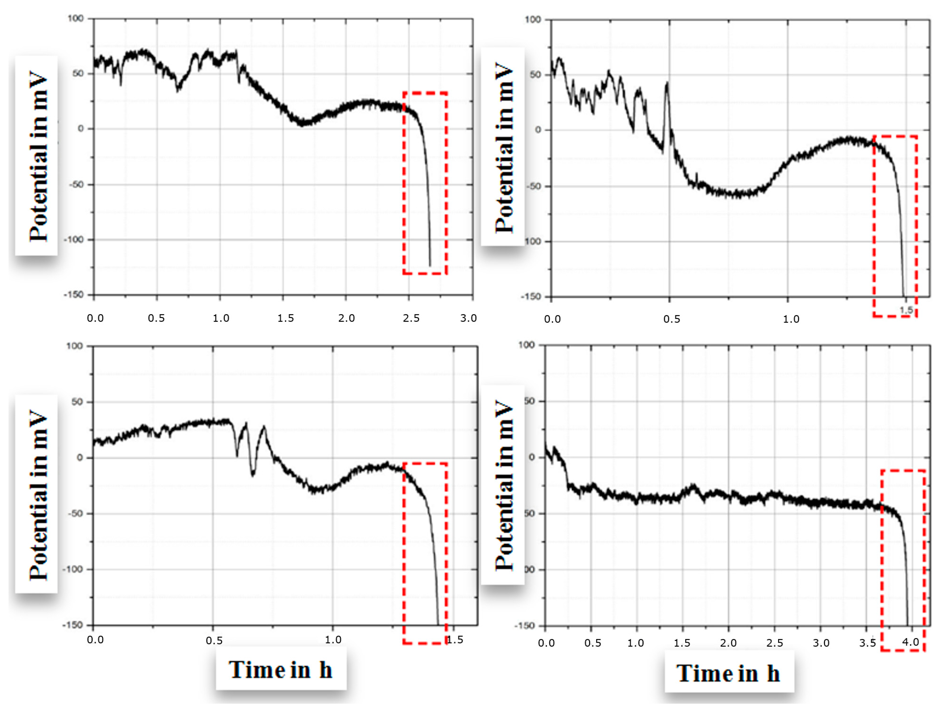
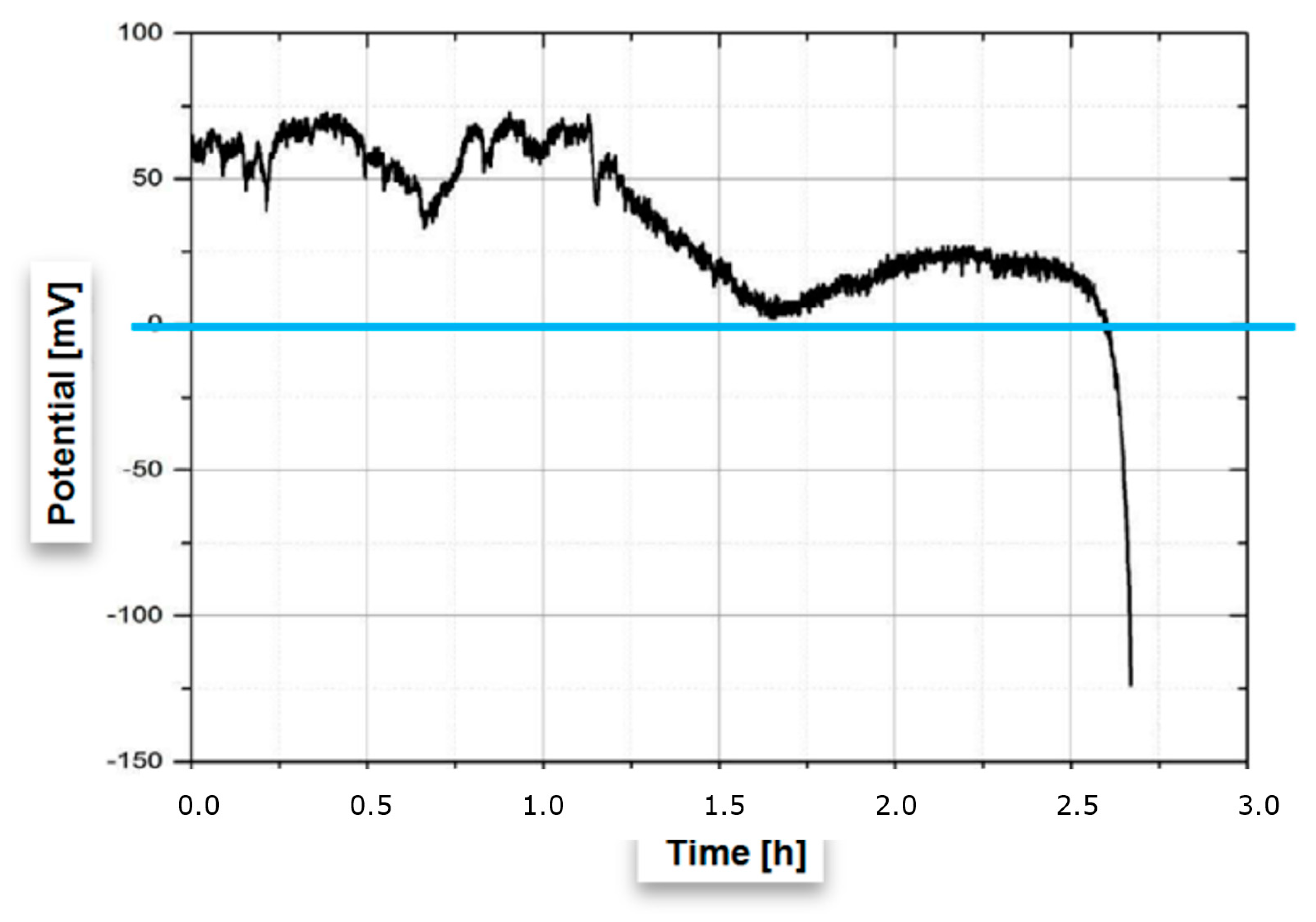
3.3. Estimating Early Failure from Electrical Potential

The aim is to stop the fatigue testing equipment prior to failure of the specimen. After further and final evaluation, a possible algorithm might then be applied to components in geothermal power plants (e.g., pump shafts in geothermal pumps that are stopped before failure of the component and before severe damage is caused to the entire pump).

Because data points displaying the drop of the potential are measured during crack propagation, these are not valuable to determine the early onset of the failure. Therefore, there is a need to interpret the potential values immediately before crack initiation or even crack initiation itself should be detected to correlate both with the onset of failure. Datapoints are collected every five seconds, because, firstly, the number of data points was rather easy to handle; secondly, the intervals are sufficiently appropriate to detect a change in potential values, and thirdly, a sufficient high resolution of the onset of failure was reached. Depending on the potential values, each of these data points needs to be sufficient to stop the fatigue testing immediately at any time of the experiment (before crack propagation). It is non-trivial to interpret the discontinuous process of the free corrosion potential over a long period because it could easily be mistaken as the onset of crack propagation (Figure 6, right red box). Therefore, it is highly necessary to distinguish between various potential processes and only stop fatigue testing in the case of actual failure of the specimen. Figure 6 demonstrates the statistical distribution of the potential data during the drop in potential over time, highlighting the difficulty to correlate with the onset of crack propagation in the material due to discontinuous experimental data. The long-term distribution (Figure 6, right, long-term distribution), however, then reveals an onset of failure after a period of decreasing and increasing potential values (Figure 6, left, short-term distribution).

Variables such as time and frequency are independent and show no influence on endurance limit and potential for the specimen in a stable passive state (such as X2CrNiMoN22-5-3 in this case). Note that, up to this time, the failure of each specimen occurring at different times cannot be related to residual stresses, because, at high numbers of failure and low-to-moderate stress amplitudes, corrosion mechanisms clearly dominate the failure procedure. Therefore, the onset is more likely to be related to early and local corrosion phenomena rather than intrinsic mechanical properties. At 33 Hz and a maximum number of cycles set for 10⁷, the experiments last 84.175 h (3.5 days) (at frequency 33 Hz: 33 numbers of cycles per second equals 303,030.3 s for 10⁷ numbers of cycles) (Equation (1)).

$$\begin{gathered} D_V={\displaystyle \frac{N}{f}} \\ {D}_V={\displaystyle \frac{\mathrm{10,000,000}}{33 }}=\underset{\_}{\underset{\_}{303030.3}} \end{gathered}$$

(1)

• $D_V=test durance$
• $f=frequency$
• $N=number of cycles to failure$.

Data points are taken every five seconds resulting in a maximum number of data points of 60,606 according to Equation (2).

$$\begin{gathered} M_w=\frac{D_v}{5} \\ {M}_w=\frac{303030.3}{5}=\underset{\_}{\underset{\_}{60606}} \end{gathered}$$

(2)

$M_w=number of data points$.

Because one single data point (out of more than 60,000) is not significant to determine failure, time series offer a possible and sensible solution. Moreover, time series can be displayed as a function over time. A total of 10 time series each containing 10 data points shifted by 1 comprise all data. Calculations are only conducted with the series followed by a reset to generate the following data series. The incubation time is 10 data points (50 s with 1 data point = 5 s); after that, each data point will eventually be number 10 and calculated immediately. Because the number of data points is sufficiently small, it shows reliable validity.

Condition 1:

To ensure that fluctuations of the signal during fatigue testing do not lead to early break-off of the experiment, different trends have to be defined (Figure 7). In Figure 7, the red boxes represent upward trends and green boxes downward trends. Note that not all trends are present in every fatigue curve. Trends describe relations of data points over a period of time and not fluctuations of single data points. Differentiation in positive and negative potential is very important, because failure was initiated only in correlation with negative electrochemical potential. Therefore, all potentials and fluctuations above 0 were eliminated (Figure 8). In Figure 8, the blue line refers to the potential of 0.

The example given in Figure 7 shows that 250 s are left to end the experiment before the testing machine will stop its program. This is defined as sufficient to take action giving the time advantage. However, crack initiation may only be defined by fluctuations in frequency from the testing machine which then is no longer possible to observe. Also, this rule only applies for one test setup (time, temperature, pressure, atmosphere, and fluid aquifer).

Condition 2:

Single data points are random values and show strong statistical distribution. Therefore, the arithmetic mean is calculated according to Equation (3) once the time course is completed. This reduces the number of data points by a factor of 10, smoothing the distribution of data points. Arithmetic means are calculated for all time courses completed with negative numbers.

$${\overline{y}}_j={\displaystyle \frac{1}{n}}\sum _{i=1}^n{y}_i$$

(3)

• $n=number of data points$
• ${\overline{y}}_j=arithmetic mean of particular time course$
• $y_i=data point of a single time course$
• $j=number of time course$
• $i=number of data point within time course$

Arithmetic means define the trend as follows: the balance of time courses according to Equations (4)–(6) show upwards or downwards trends.

$$∆y={\overline{y}}_1-{\overline{y}}_2$$

(4)

$$⋮$$

$$∆y={\overline{y}}_9-{\overline{y}}_{10}$$

(5)

$$∆y={\overline{y}}_{10}-{\overline{y}}_1$$

(6)

If the difference values are constantly positive over a certain period of time, they indicate a downwards trend (zero is interpreted as a positive value). Negative difference values would indicate an upwards trend but are without meaning because, as stated above, the data points greater than zero are not related to failure of the fatigue sample. In the case of eliminated marked time courses, the balances were also eliminated.

In general, negative balances could be neglected in trends. However, here they serve as another condition: the 10 following balances have to be greater than the preceding balance over a period of 50 s. Due to the statistical distribution, negative balances also occur during the failure process of the sample and serve as intermission (Figure 9). Figure 9 shows a representative set of data where a negative balance divides data sets. These are only slightly visible in the curve.

To prevent intermissions, another 10 balances are generated once 10 positive balances are completed to delay the final intermission allowing for more conditions during the 50 s period. Therefore, the second condition can newly be fulfilled after each intermission.

Condition 3:

The third condition comprises the calculation of the gradient (m) and the coefficient of determination (R²) of each time course after fulfillment of condition 2. The gradient describes the intensity of the direction of the trend. The coefficient of determination allows for data points to be described as a function [28,29]; here, a polynomial of first degree or a best-fit straight line is appropriate. The gradient is determined via the least square method (Equation (7)).

$$m={\displaystyle \frac{{\sum }_{i=1}^n(x_i-{\overline{x}}_j)·(y_i-{\overline{y}}_j)}{{\sum }_{i=1}^n{(x_i-{\overline{x}}_j)}^2}}$$

(7)

• $m=gradient$
• $x_i=number of data points within time course \left(1 to 10\right)$
• ${\overline{x}}_j=arithmetic mean of numbers$
• $y_i=data point of time course$
• ${\overline{y}}_j=arithmetic mean of time course$

Because the consecutive numbering of data points as x-values is consistent in all time courses the following simplification is possible (Equation (8)):

• The arithmetic mean of numbering is ${\overline{x}}_j$= 5.5 for the mean of time courses 1 to 10;
• ${\sum }_{i=1}^n{(x_i-{\overline{x}}_j)}^2$ is the distance between x-values and the arithmetic mean of numbering of the particular time course with respect to the Cartesian grid to the second power. Because the numbering remains the same in each time course, it contributes as a constant to simplify Equation (7) to calculate the gradient. Inserting numbers 1 to 10, the gradient is 82.5.

$$m={\displaystyle \frac{{\sum }_{i=1}^n(x_i-5.5)·(y_i-{\overline{y}}_j)}{82.5}}$$

(8)

Equation (9) gives the calculation of the coefficient of determination (R²).

$$R^2={\left({\displaystyle \frac{{\sum }_{i=1}^n(x_i-{\overline{x}}_j)·(y_i-{\overline{y}}_j)}{\sqrt{{\sum }_{i=1}^n{(x-{\overline{x}}_j)}^2·{\sum }_{i=1}^n{(y_i-{\overline{y}}_j)}^2}}}\right)}^2$$

(9)

The simplification for determining the gradient also applies for the coefficient of determination (R²) (Equation (10)).

$$R^2={\left({\displaystyle \frac{{\sum }_{i=1}^n(x_i-5.5)·(y_i-{\overline{y}}_j)}{\sqrt{82.5·{\sum }_{i=1}^n{(y_i-{\overline{y}}_j)}^2}}}\right)}^2$$

(10)

To fulfill condition 3, condition 1 and 2 have to be fulfilled. The gradient is set for m ≤ −1 (subcondition 1) and is sufficiently high so that times courses only apply at the end of the endurance test. The coefficient of determination (R²) is set for R² ≥ 0.8 (subcondition 2). This only occurs for time courses where most values are smaller than their precursor, so that these only scatter slightly from the partial regression line.

The necessary conditions may be summarized as follows:

Condition 1

• Each data point is compared to zero;
• For positive values, the time course is marked;
• After completion of 10 positive values, the time course is eliminated and not evaluated;
• Only fully negative data series are evaluated.

Condition 2

• Arithmetic means are calculated for all time courses completed with negative num-bers (non-marked);
• Balances of arithmetic mean values are calculated giving a trend for balance ≥ 0 (zero is interpreted as positive value);
• Intermission for ≥10 positive balances leads to a delay in data points.

Condition 3

• Conditions 1 and 2 need to be fulfilled;
• Gradient (m) and coefficient of determination (R²) immediately after fulfillment of condition 2;
• m ≤ −1;
• R² ≥ 0.8;
• Two sub-conditions need to be fulfilled;
• Determination of experiment for three consecutive time courses applying to both sub-conditions.

Sub-condition 1

• If m ≤ −1, mark the time course;
• If m ≥ −1, reset.

Sub-condition 2

• If R² ≥ 0.8, mark the time course;
• If R² ≤ 0.8 reset.

During a first test run, the algorithm was reliable for 14 out of 15 specimens giving a functional probability of 93.3%. Greater reliability may be achieved by adapting the boundary conditions and will be subject to further research.

4. Conclusions

Predicting early failure based on the electrochemical potential of steel subjected to both highly corrosive environments and mechanical stress could significantly lower maintenance needs and reduce costs in geothermal energy production facilities.

The corrosion fatigue behavior of hour-glass shaped specimens of duplex stainless-steel X2CrNiMoN22-5-3 was investigated in an individual test set-up. Artificial thermal water as the corrosive medium setting the geothermal environment of the Northern German Basin was heated to 369 K. The electric potential of an in-house manufactured Ag/AgCl wire electrode was measured versus the reference Ag/AgCl glass electrode, and failure of corrosion fatigue specimens in CCS environment was correlated with the drop of the curves of the electrochemical potential.

The measured potential values were divided into ten time series, each containing ten data points, to establish a test algorithm. This process combined splitting with calculations of mean values, slopes, and regressions, successfully initiating the algorithm. Time courses consisting of ten consecutive numbers, drawn every five seconds, were analyzed under three main conditions and two sub-conditions. The algorithm’s functionality was evaluated using fifteen potential functions.

During the initial test run, the algorithm demonstrated reliability for 14 out of 15 specimens, achieving a functionality level of approximately 93%, with a predictive time lead of up to 435 s. These findings suggest that it is feasible to predict corrosion fatigue failure in test specimens under geothermal conditions—similar to those in geothermal energy production—using in situ electrochemical potential measurements. In the future, refinement of the algorithm will focus on improving the reliability to a higher percentage.

An algorithm predicting early failure during corrosion fatigue can enhance the reliability and safety of geothermal energy production and carbon capture and storage (CCS) sights by enabling proactive maintenance and reducing the risk of unexpected equipment failure. This predictive capability minimizes downtime and operational costs while extending the lifespan of critical infrastructure exposed to highly corrosive geothermal or CCS conditions. Additionally, it supports sustainable energy practices by ensuring consistent system performance and mitigating environmental risks associated with material degradation.

References

1. Thomas, J.P.; Wei, R.P. Corrosion fatigue crack growth of steels in aqueous solutions I: Experimental results and modeling the effects of frequency and temperature. Mater. Sci. Eng. 1992, 159, 205–221. [Google Scholar] [CrossRef]
2. Mu, L.J.; Zhao, W.Z. Investigation on Carbon Dioxide Corrosion Behaviors of 13Cr Stainless Steel in Simulated Strum Water. Corros. Sci. 2010, 2, 82–89. [Google Scholar] [CrossRef]
3. Unigovski, Y.B.; Lothongkum, G.; Gutman, E.M.; Alush, D.; Cohen, R. Low-cycle fatigue behavior of 316L-type stain-less steel in chloride solutions. Corr. Sci. 2009, 51, 3014–3120. [Google Scholar] [CrossRef]
4. Holtam, C.M.; Baxter, D.P.; Ashcroft, I.A.; Thomson, R.C. Effect of crack depth on fatigue crack growth rates for a C–Mn pipeline steel in a sour environment. Int. J. Fatigue 2010, 32, 288–296. [Google Scholar] [CrossRef]
5. Thorbjörnsson, I. Corrosion fatigue testing of eight different steels in an Icelandic geothermal environment. Mater. Des. 1995, 16, 97–102. [Google Scholar] [CrossRef]
6. Pfennig, A.; Wolf, M.; Heynert, K.; Böllinghaus, T. First In-Situ Electrochemical Measurement During Fatigue Testing of In-jection Pipe Steels to Determine the Reliability of a Saline Aquifer Water CCS-Site in the Northern German Basin Original. Energy Procedia 2014, 63, 5773–5786. [Google Scholar] [CrossRef]
7. Zhang, W.; Fang, K.; Hua, Y.; Wang, S.; Wang, X. Effect of machining-induced surface residual stress on initiation of stress corrosion cracking in 316 austenitic stainless steel. Corros. Sci. 2016, 108, 173–184. [Google Scholar] [CrossRef]
8. Evgeny, B.; Hughes, T.; Eskin, D. Effect of surface roughness on corrosion behaviour of low carbon steel in inhibited 4 M hydrochloric acid under laminar and turbulent flow conditions. Corros. Sci. 2016, 103, 196–205. [Google Scholar] [CrossRef]
9. Xu, M.; Zhang, Q.; Yang, X.X.; Wang, Y.; Liu, J.; Li, Z. Impact of surface roughness and humidity on X70 steel corrosion in su-percritical CO2 mixture with SO2, H2O, and O2. J. Supercrit. Fluids 2016, 107, 286–297. [Google Scholar] [CrossRef]
10. Lee, S.M.; Lee, W.G.; Kim, Y.H.; Jang, H. Surface roughness and the corrosion resistance of 21Cr ferritic stainless steel. Corros. Sci. 2012, 63, 404–409. [Google Scholar] [CrossRef]
11. Ahmed, A.A.; Mhaede, M.; Basha, M.; Wollmann, M.; Wagner, L. The effect of shot peening parameters and hydroxyapatite coating on surface properties and corrosion behavior of medical grade AISI 316L stainless steel. Surf. Coat. Technol. 2015, 280, 347–358. [Google Scholar] [CrossRef]
12. Kleemann, U.; Zenner, H. Structural component surface and fatigue strength—Investigations on the effect of the surface layer on the fatigue strength of structural steel components. Mater. Werkst. 2006, 37, 349–373. [Google Scholar] [CrossRef]
13. Sanjurjo, P.; Rodríguez, C.; Pariente, I.; Belzunce, F.; Canteli, A. The influence of shot peening on the fatigue behaviour of duplex stainless steels. Procedia Eng. 2010, 2, 1539–1546. [Google Scholar] [CrossRef]
14. Abdulstaar, M.; Mhaede, M.; Wollmann, M.; Wagner, L. Investigating the effects of bulk and surface severe plastic deformation on the fatigue, corrosion behaviour and corrosion fatigue of AA5083. Surf. Coat. Technol. 2014, 254, 244–251. [Google Scholar] [CrossRef]
15. Wu, X.; Guan, H.; Han, E.H.; Ke, W.; Katada, Y. Influence of surface finish on fatigue cracking behavior of reactor pressure vessel steel in high temperature water. Mater. Corros. 2006, 57, 868–871. [Google Scholar] [CrossRef]
16. Alvarez-Armas, I. Duplex Stainless Steels: Brief History and Some Recent Alloys. Recent Pat. Mech. Eng. 2008, 1, 51–57. [Google Scholar] [CrossRef]
17. Schultze, S.; Göllner, J.; Eick, K.; Veit, P.; Heyse, H. Selektive Korrosion von Duplexstahl. Teil 1: Aussagekraft herkömmlicher und neuartiger Methoden zur Untersuchung des Korrosionsverhaltens von Duplexstahl X2CrNiMoN22-5-3 unter besonderer Berücksichtigung der Mikrostruktur. Mater. Corros. 2010, 52, 26–36. [Google Scholar] [CrossRef]
18. Prosek, T.; Le Gac, A.; Thierry, D.; Le Manchet, S.; Lojewski, C.; Fanica, A.; Johansson, E.; Canderyd, C.; Dupoiron, F.; Snauwaert, T.; et al. Low-Temperature Stress Corrosion Cracking of Austenitic and Duplex Stainless Steels Under Chloride Deposits. Corrosion 2014, 70, 1052–1063. [Google Scholar] [CrossRef]
19. Pfennig, A.; Wolf, M.; Kranzmann, A. Corrosion and Corrosion Fatigue of Steels in Downhole CCS Environment—A Summary. Processes 2021, 9, 594. [Google Scholar] [CrossRef]
20. Wolf, M. Phänomenologie der Schwingungsrisskorrosion von austenitisch-ferritischen Duplexstählen in hoch salzhaltigen wässrigen Lösungen. Ph.D. Thesis, University OVG Magdeburg, Magdeburg, Germany, 2018. [Google Scholar]
21. Wolf, M.; Pfennig, A. Deriving early corrosion fatigue failure of steels from frequency drop and electrochemical potential. In Proceedings of the 8th International Conference on Materials Sciences and Nanomaterials (ICMSN 2024), Edingburgh, UK, 9–12 July 2024. [Google Scholar]
22. DIN EN ISO 11782-1:2008-08; Corrosion of Metals and Alloys—Corrosion Fatigue Testing—Part 1: Cycles to Failure Testing (ISO 11782-1:1998); German version EN ISO 11782-1:2008. ISO: Geneva, Switzerland, 2008.
23. Förster, A.; Norden, B.; Zinck-Jørgensen, K.; Frykman, P.; Kulenkampff, J.; Spangenberg, E.; Erzinger, J.; Zimmer, M.; Kopp, J.; Borm, G.; et al. Baseline characterization of the CO2SINK geological storage site at Ketzin, Germany. Environ. Geosci. 2006, 13, 145–161. [Google Scholar] [CrossRef]
24. Forster, A.; Schoner, R.; Förster, H.-J.; Norden, B.; Blaschke, A.-W.; Luckert, J.; Beutler, G.; Gaupp, R.; Rhede, D. Reservoir characterization of a CO2 storage aquifer: The Upper Triassic Stuttgart Formation in the Northeast German Basin. Mar. Pet. Geol. 2010, 27, 2156–2172. [Google Scholar] [CrossRef]
25. Bäßler, R.; Sobetzki, J.; Klapper, H.S. Corrosion resistance of high-alloyed materials in artificial geothermal fluids. In NACE International Corrosion Conference Series, Proceedings of the Corrosion 2013, Orlando, FL, USA, 17–21 March 2013; Paper No. 2327; NACE Corrosion Conference & Expo: Orlando, FL, USA, 2013. [Google Scholar]
26. Cammann, K.; Galster, H. Das Arbeiten Mit Ionenselektiven Elektroden; Springer: Berlin/Heidelberg, Germany, 1977. [Google Scholar]
27. Baucke, F.G.K. Standardpotentiale der Silber/Silber-Chlorid-Elektrode in 3,5 m und in ges. KCl Unter Verwendung Entsprechender (“Cl-Ionensensitiver”) Membranelektroden (0–95 °C). Chemie Ing. Tech. CIT 1975, 47, 565–566. [Google Scholar] [CrossRef]
28. Kuckartz, U.; Rädiker, S.; Ebert, T.; Schehl, J. Statistik: Eine verständliche Einführung, 1st ed.; Springer Fachmedien: Wiesbaden, Germany, 2010; pp. 233–238. ISBN 978-3-531-16662-9. [Google Scholar]
29. Hüftle, M. Modelle und Methoden der Zeitreihenanalyse; Universität Hannover: Hannover, Germany, 2006. [Google Scholar]
Figure 1. Test specimen for fatigue experiments with actual sample in schematic drawing.
Applsci 15 00403 g001
Figure 2. Corrosion chamber for axial load and possible measurement access spots.
Applsci 15 00403 g002
Figure 3. Schematic setup of the in situ corrosion fatigue testing procedure and electrochemical data collection. The setup with respect to different aspects has been used and described earlier [19,20].
Applsci 15 00403 g003
Figure 4. Test setup and electric potential of the Ag/AgCl wire electrode in relation to the SHE; the value of the Ag/AgCl glass electrode was adopted from [6,20].
Applsci 15 00403 g004
Figure 6. Demonstration of statistical distribution of the potential data of X2CrNiMoN22-5-3 measured via an Ag/AgCl wire electrode (left: short term distribution; right: long term distribution).
Applsci 15 00403 g006
Figure 7. Grouping trends of the statistically distributed potential data of X2CrNiMoN22-5-3 (Ag/AgCl wire electrode, insulated fatigue test setup). Red boxes: upward trends; green boxes: downward trends.
Applsci 15 00403 g007
Figure 8. Example of elimination of potential data > 0 of X2CrNiMoN22-5-3 (Ag/AgCl wire electrode, insulated fatigue test setup). All potentials and fluctuations above 0 were eliminated.
Applsci 15 00403 g008
Figure 9. Example of failure phase and interruption of X2CrNiMoN22-5-3 (Ag/AgCl wire electrode, insulated fatigue test setup) after 2,350,268 cycles to failure.
Applsci 15 00403 g009