Recurrent Deep Learning for Beam Pattern Synthesis in Optimized Antenna Arrays

Abstract

This work proposes and describes a deep learning-based approach utilizing recurrent neural networks (RNNs) for beam pattern synthesis considering uniform linear arrays. In this particular case, the deep neural network (DNN) learns from previously optimized radiation patterns as inputs and generates complex excitations as output. Beam patterns are optimized using a genetic algorithm during the training phase in order to reduce sidelobes and achieve high directivity. Idealized and test beam patterns are employed as inputs for the DNN, demonstrating their effectiveness in scenarios with high prediction complexity and closely spaced elements. Additionally, a comparative analysis is conducted among the three DNN architectures. Numerical experiments reveal improvements in performance when using the long short-term memory network (LSTM) compared to fully connected and convolutional neural networks.

1. Introduction

The use of antenna arrays in wireless communication systems has proven to be a key design parameter for performance improvement [1]. Broadcast satellite communication, point-to-point communication, radar systems, and mobile communication systems suffer from problems such as interference, scattering, and attenuation that may severely affect long-distance communications [1,2]. Thus, antenna arrays consisting of a set of radiators that are capable of providing advanced features to generate one or several beams with different shapes toward a specific user or region are used, thus improving the system’s capacity and efficiency. These capabilities are valuable in scenarios where high data rates are required. Antenna arrays make techniques such as beamforming and multiple-input multiple-output (MIMO) possible, which are expected to play significant roles in 6G systems and beyond [3].

Beam pattern synthesis usually refers to the controlled generation of radiation patterns by antenna arrays. These beam patterns are designed to direct signal energy in a specific manner, enhancing signal reception or transmission in a particular direction while minimizing it in others. Thus, the synthesis process typically involves both manipulating the antenna array’s geometry and complex excitations (amplitudes and phases) of individual antenna elements.

Classical iterative methods to solve the problem of beam pattern synthesis exist and are typically categorized as either local or global optimizers, with some of them being based on Fourier transforms [4,5]. Nevertheless, despite their proven reliability and robustness, a vast majority of these methods require considerable computational time, being dependent on the synthesis of a large number of radiation patterns. Other traditional optimization methods, such as evolutionary algorithms for beam pattern synthesis in uniform linear antenna arrays, have notable drawbacks, such as high computation costs [6,7], sensitivity to parameters [6,8], and convergence issues [9]. To address these challenges, alternative approaches are often pursued.

In recent years, innovative deep learning (DL) approaches have permeated numerous research areas and practical applications. This trend is primarily attributed to advancements in the development of specialized hardware, such as GPUs, along with improvements in neural network algorithms and the availability of vast datasets for training these systems [10]. With its remarkable progress, this technology has made significant strides across diverse fields, showcasing notable success in areas such as computer vision, natural language processing, speech recognition, healthcare, robotics, recommendation systems, financial modeling, climate science, bioinformatics, material inspection, and quality control [11,12]. Furthermore, there are other areas, such as electromagnetic (EM) problems [13], where its recent integration has been observed. In this context, DL methodologies have emerged as a pivotal tool for synthesizing and designing a variety of configurations and types of antennas [14].

In antenna characterization, DL techniques have proven to be quite useful for reducing the number of EM simulations, which are generally computationally expensive [15]. In the same way, DL approaches have been successfully applied to various antenna problems, including antenna synthesis [16,17].

The ability to synthesize beam patterns through machine learning techniques—particularly support vector machines (SVM) and artificial neural networks (ANN)—has previously been demonstrated [14,18]. However, these methodologies have inherent limitations in terms of learning different beam patterns; specifically, ANNs without the use of deep hidden layers may be unable to provide antenna design parameters for arbitrary antenna beam patterns [19]. On the other hand, it is noteworthy that a large majority of DL methodologies proposed to solve these types of electromagnetic problems are based on convolutional neural networks (CNNs or ConvNets) [20]. Thus, various studies have proposed deep convolutional neural network architectures with eight layers in different configurations. In [21], a method for two-dimensional synthesis of a reflectarray with a circular aperture to predict the phase shift was presented. This study employed five convolutional layers (CLs) and three fully connected layers (FCLs). Similarly, another study proposed a different CNN with four CLs and four FCLs, which was trained to obtain the phases of an $8\times 8$ patch antenna array with a two-dimensional radiation pattern as an input [22]. Additionally, in reference [23], other authors proposed a CNN architecture with five CLs and three FCLs to determine the complex excitations of a planar array with circular aperture. Their focus was on maximizing only the directivity, doing so with a fixed constraint mask on the side lobes.

This article introduces a novel deep learning-based approach using a long short-term memory neural network for antenna synthesis. Our contribution involves calculating complex excitations in response to ideal input radiation patterns with beam patterns featuring reduced sidelobes and high directivity. The proposed DL methodology is also extended to attainable and fixed radiation patterns.

The remainder of this paper is organized as follows: Section 2 addresses linear array optimization and deep neural network modeling, while Section 3 presents the antenna pre-synthesis process, data arrangement, pre-processing, and results obtained with the considered DNNs. Finally, in Section 5, the conclusions of this work are presented.

2. Problem Formulation

2.1. Antenna Array Optimization

Let us consider a linear array configuration comprising N omnidirectional antenna elements within the azimuthal plane ($xy$ plane). Its array factor ($AF\left(\theta \right)$) for a collection of arbitrary inputs [$\mathit{I}$] is given by [24]:

$$AF(\theta ,\mathit{I})=\sum _{n=1}^N{I}_{n}exp[jk{d}_{n}cos\theta -{\alpha }_n],$$

(1)

where $I_n$ denotes the complex weights ($I_n=A_n{e}^{j{\xi }_n}$, where ${\xi }_n\in [0,180])$ of the n-th radiator of the array, k is the wavenumber, $d_n$ is the position of the radiator n, and ${\alpha }_n=k{d}_{n}cos{\theta }_0$ is a phase delay related to the peak directivity attained (${\theta }_0$).

In this work, the beam pattern synthesis problem consists of generating a beam pattern with minimum sidelobe level (SLL) and maximum directivity (D) in a pre-defined direction of interest. Then, the beam pattern obtained from the optimization process is taken as input by the DNNs under study. To attain the aforementioned pre-determined design characteristics, the associated synthesis issue can be mathematically formulated as a constrained optimization problem in the following manner [24]:

$$\begin{array}{cccc}\hfill & \underset{\mathit{I}}{min}\hfill & \hfill & \left\{{\displaystyle \frac{\left|AF\right({\varphi }_{SL},\mathit{I}\left)\right|}{\left|AF\right({\varphi }_{max},\mathit{I}\left)\right|}}\right\}+\left\{{\displaystyle \frac{1}{D(\varphi ,\mathit{I})}}\right\}\hfill \\ \hfill & \mathrm{s}.\mathrm{t}.\hfill & \hfill & \left|AF\right({\varphi }_{max},\mathit{I}\left)\right|=1,\hfill \\ \hfill & \hfill & & \mathit{I}=\left\{A_n{e}^{j{\xi }_n}\right|\mathit{I}\in \mathbb{I}\},\forall n\in N.\hfill \end{array}$$

(2)

In (2), ${\varphi }_{SL}$ denotes the angle where the maximum sidelobe is achieved on either side of the main lobe, ${\varphi }_{max}$ represents the main beam direction, and $\mathbb{I}$ is the amplitude and phase domain. Moreover, given the degrees of freedom and the intricate nature of antenna synthesis optimization, a classic metaheuristic approach based on evolutionary computation is employed, and the setup is detailed in the following.

2.2. Deep Neural Network Modeling

To address the challenge of predicting amplitudes and phases from pre-optimized radiation patterns, we situated the problem within the framework of supervised learning, conceptualizing it as a predictive task due to the continuous nature of the provided amplitudes and phases. Unlike classification tasks that deal with discrete values, regression—a subtype of supervised learning—is adept at handling continuous labels. In regression, the objective is to learn a mapping from input features to continuous output values, enabling the model to predict numerical quantities based on input data. To address this regression problem, we explored the utilization of three widely recognized neural network architectures: fully connected neural networks (FCNNs), convolutional neural networks (CNNs), and long short-term memory networks (LSTMs). Each architecture offers unique capabilities suited to different types of data and tasks, facilitating the learning of intricate relationships between the input features extracted from radiation patterns and the continuous output labels of amplitudes and phases.

In a densely connected neural network or FCNN, each neuron within a layer is coupled to every neuron in the following layer, facilitating the flow of information from the input layer to the output layer as it sequentially traverses each intermediate layer. In each layer, the network calculates a weighted sum of the inputs and their associated weights, incorporating non-linear activation functions to introduce complexity and enable the model to capture intricate patterns in the data. This iterative process continues until the information reaches the output layer, where the network generates its prediction based on the learned relationships encoded in the network’s parameters. The fully connected architecture offers versatility and can effectively learn complex mappings between inputs and outputs, making it well-suited for a variety of tasks in machine learning and deep learning domains [25].

A convolutional neural network (CNN) typically comprises convolutional, pooling, and fully connected layers. Convolutional layers are crucial in performing cross-correlation operations, acting as feature extractors. Pooling layers down-sample and reduce the dimension of the network’s features, often through performing max-pooling operations. While leading to some information loss, these layers mitigate the risk of over-fitting, enhance efficiency, and reduce complexity. In a CNN, there is a sequential arrangement of convolutional and pooling layers; however, we do not report the pooling layers for this task, as they did not improve the employed CNN. The fully connected layers generate the output, which predicts the labels using the features extracted by the preceding layers [26]. Typically, CNNs are used on two-dimensional signals (2D-CNN); however, in this study, we used one-dimensional signals due to the nature of the radiation patterns (1D-CNN).

A long short-term memory (LSTM) is a recurrent neural network (RNN) architecture designed to handle long-term sequential data and dependencies. LSTMs improve the limitations of conventional RNNs by adding memory cells that are capable of retaining information over extended periods. These architectures comprise memory cells with input, output, and forget gates. The memory cells store and update information, while the gates regulate the flow of information within the network; in particular, the input gate controls the information entering the memory cells, the forget gate determines which information to discard, and the output gate decides which information to output from the memory cells [27].

Figure 1 illustrates the three deep neural network architectures devised for predicting amplitude and phase in radiation patterns. These offer great flexibility and their usefulness and reliability across various problems have been demonstrated over the decades. It is worth noting that meticulous optimization of these architectures was conducted through the systematic tuning of hyperparameters, including but not limited to the number of layers, neurons, activation functions, and learning rate, among others. Algorithm 1 shows the general procedure used to train the different proposed architectures. This algorithm outlines the process of training a neural network using gradient descent optimization to minimize the mean squared error (MSE) loss function. It involves iterating through the training data multiple times (epochs) and updating the model parameters (weights and biases) after each mini-batch based on the calculated gradients. The goal is to fine-tune the model’s parameters in order to reduce the prediction error and enhance the performance of the neural network when analyzing the training data. These architectures were implemented using the Keras framework [28].

Algorithm 1 Training algorithm

Input: Training set $\left(\mathbf{X},\mathbf{Y}\right)$ $\mathbf{ff}\leftarrow \alpha$//Initialize learning rate $\mathbf{epochs}\leftarrow epochs$//Initialize the number of epochs $\mathbf{w}\leftarrow w$//Initialize weights $\mathbf{b}\leftarrow b$//Initialize bias For each iteration in epochs Do     Shuffle and split training set $(\mathbf{X},\mathbf{Y})$     For each mini-batch $({\mathbf{X}}_i,Y_i)$ Do        Perform forward pass//Predict amplitudes and phases        Perform MSE $({\mathbf{Y}}_i,{\widehat{Y}}_i)$//Predict error        Compute $\nabla w$//w gradients        Compute $\nabla b$//b gradients     $w\leftarrow w-\alpha \nabla w$ //Update weights     $b\leftarrow b-\alpha \nabla b$ //Update bias Output: Trained neural network

Two metrics were used to assess the performance of the deep neural network architectures. The first metric was the mean absolute error (MAE), which measures the absolute error between the desired label and the label predicted by the neural network:

$$\mathrm{MAE}={\displaystyle \frac{{\sum }_{i=1}^n|y_i-{\widehat{y}}_i|}{n}}.$$

(3)

The second metric was the mean square error (MSE), which evaluates the quadratic error between the desired and predicted labels:

$$\mathrm{MSE}={\displaystyle \frac{1}{n}}\sum _{i=1}^n{(y_i-{\widehat{y}}_i)}^2,$$

(4)

where $y_i$ is the desired label, ${\widehat{y}}_i$ is the predicted label, and n is the number of patterns.

3. Numerical Experiments

3.1. Antenna Pre-Synthesis Process

In this study, preliminary beam pattern synthesis in the antenna system was achieved using genetic algorithms, which explore multiple combinations of potential solutions to identify a quasi-optimal solution for an equally spaced linear antenna array in order to fulfill specific objectives prior to training the DNN. GAs are robust and trustworthy evolutionary algorithms categorized as population-based optimizers, which have been extensively used on electromagnetics problems, including beam pattern synthesis and antenna design.

A GA approach was utilized to assess the array factor across the azimuthal plane within a window spanning $(50°\le \theta \le 130°)$. The training data’s radiation patterns were obtained by incrementing the phase by 20°. The number of instances generated per angle was 847, resulting in a total of 7623 radiation patterns. As a case study, a uniform antenna array with a linear geometry consisting of 8 equidistant elements spaced at intervals of $d=0.5 \lambda$ was employed (Figure 2). The approach used standard genetic operators [29], including a selection method that combines fitness ranking and elitist selection, as well as two-point crossover ($P_c=1.0$). Additionally, a single mutation operation was applied ($P_m=0.1$), wherein a locus was randomly selected, and the allele was replaced with a random number uniformly distributed within the feasible region of the search space. The GA algorithm begins by initializing a population comprising 250 individuals, all subjected to 500 iterations, ensuring comprehensive sampling of the solution space. In this work, the GA approach was implemented using MATLAB R2019b.

3.2. Data Arrangement and Pre-Processing for DNN

A total of 7623 radiation patterns were generated for training and arranged into a matrix $X\in {\mathbb{R}}^{7623\times 180}$, 32 patterns for validation $X\in {\mathbb{R}}^{32\times 180}$, and 92 patterns for testing $X\in {\mathbb{R}}^{92\times 180}$, where each radiation pattern was composed of 180 features and each feature represents a point of the normalized power ranging from 1 to 180 degrees; see Figure 3. Conversely, labels for training were organized in a matrix $Y\in {\mathbb{R}}^{7623\times 16}$, for validation $Y\in {\mathbb{R}}^{32\times 16}$, and for testing $Y\in {\mathbb{R}}^{92\times 16}$, where the first eight features belonged to the amplitude of the radiation patterns and the other eight to the phase features. Note that the amplitude and phase information is embedded in the array factor that generates the radiation pattern.

3.3. Deep Neural Network Results

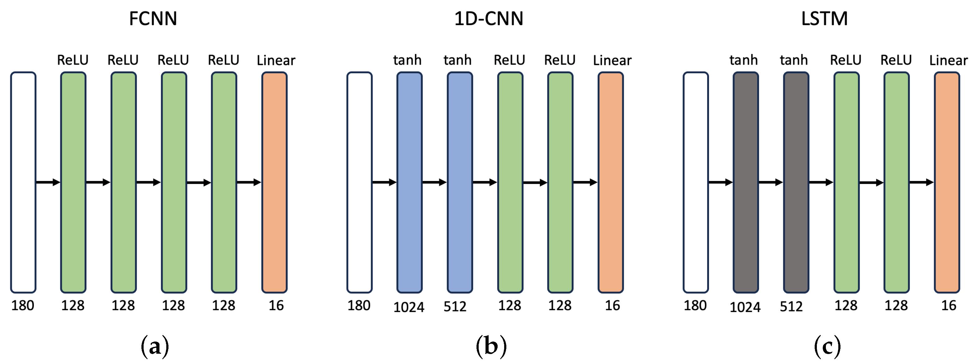
Subsequently, we employed an FCNN, a 1D-CNN, and a LSTM deep neural network to predict the amplitudes and phases of the radiation patterns. The loss function utilized was the MSE, which was used to compute the error. Furthermore, the Adam optimizer algorithm was employed for training the networks, which leverages previous gradient information and accelerates convergence [30], with a learning rate of 0.001 for 400 epochs and with mini-batches of 32 radiation patterns.

Table 1. Performance of the three proposed architectures. The best results are noted in bold.

Architecture	MAE Training	MAE Validation	MSE Training	MSE Validation
FCNN	0.2177	0.2068	0.0667	0.0601
1D-CNN	0.2177	0.2078	0.0667	0.0606
LSTM	0.0143	0.0098	3.5220$\times {10}^{-4}$	1.6166$\times {10}^{-4}$

shows the MAE and MSE values achieved by the three proposed architecture.

The LSTM outperformed the FCNN and 1D-CNN due to its ability to selectively retain or forget information based on the context and relevance of the radiation patterns. This enables the LSTM to effectively capture long-term dependencies in sequential data, making them well-suited for natural language processing, speech recognition, and time-series analysis.

On average, training with the LSTM took 7.991 min, while testing took 0.072 s for the 92 test patterns. The whole set of experiments in this paper was executed using a workstation with an Intel(R) Xeon(R) CPU @ 2.00 GHz processor with 64 GB of RAM (ASUS, León, Mexico), as well as an Nvidia RTX 3090 graphical processing unit (Nvidia, León, México).

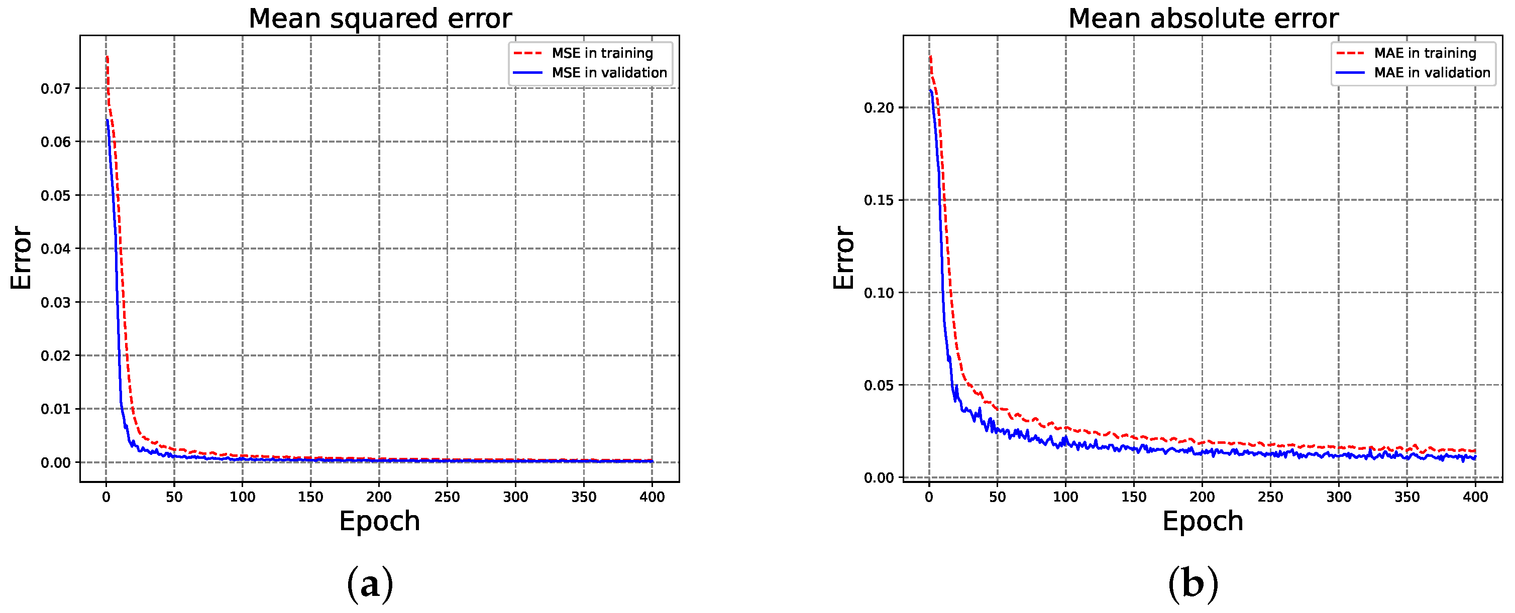
In terms of neural networks, Figure 4 illustrates that, as the training epochs progressed, the LSTM network increasingly improved its approximation of the radiation patterns to match their respective labels, including both magnitudes and phases. This process resulted in progressively smaller errors over time, with the network ultimately converging at epoch 400 for the MSE (4) and MAE (3) metrics.

On the other hand, in terms of beam pattern synthesis, the achieved errors represent the network’s capability to meet essential design requirements. During the pre-synthesis or pre-conditioning phase, we used a genetic algorithm (GA) to ensure that the synthesized patterns aligned with key antenna specifications set by the fitness function, focusing on high directivity and controlled sidelobe levels. This GA-based pre-conditioning produced training data that meet the baseline performance thresholds, allowing the LSTM network to learn not only to approximate target radiation patterns but also to capture the specific characteristics necessary for practical beamforming. As such, the decreasing mean squared error (MSE) and mean absolute error (MAE) values shown in Figure 4 reflect the network’s convergence toward patterns that satisfy these specifications, ensuring that the final loss values are appropriate for antenna beam pattern synthesis.

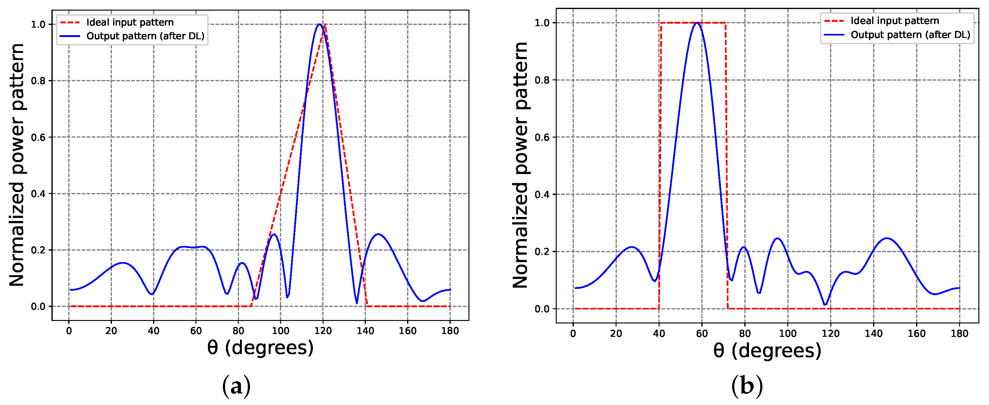
Hypothetical radiation patterns with high prediction difficulty were generated as input to the DNN with better performance (i.e., the previously trained and validated LSTM), resulting in amplitudes and phases for the antenna array. In Figure 5, the power pattern synthesis related to these idealized patterns (i.e., radiation patterns of arbitrary shapes not produced by antenna array) is shown. Figure 5a illustrates an optimal triangular input pattern, where the base of the triangle has an angular range from 85° to 140° and the opposite vertex to the base points at 120° with a gain of one. In the same manner, a perfectly square input pattern exhibiting a unit gain within the angular span of 40° to 70° is depicted in Figure 5b.

The solutions provided by the RNN for these ideal radiation patterns are shown in

Table 2. Amplitudes and phases (output data) of the LSTM-RNN.

Number of Antenna	Triangular Pattern (Figure 5a)	Square Pattern (Figure 5b)	Test Pattern 1 (Figure 6a)	Test Pattern 2 (Figure 6b)
1:	$7.55\angle 99.55°$	$8.94\angle 82.95°$	$7.99\angle 74.92°$	$8.49\angle 104.92°$
2:	$9.04\angle 62.87°$	$8.56\angle 128.55°$	$5.79\angle 91.29°$	$8.80\angle 73.23°$
3:	$11.06\angle 75.49°$	$8.02\angle 108.07°$	$8.41\angle 59.00°$	$7.88\angle 91.96°$
4:	$6.52\angle 69.78°$	$7.19\angle 90.36°$	$6.27\angle 91.80°$	$6.59\angle 80.65°$
5:	$8.70\angle 93.20°$	$10.73\angle 101.71°$	$8.19\angle 105.79°$	$8.44\angle 96.91°$
6:	$5.29\angle 91.71°$	$8.29\angle 70.66°$	$8.54\angle 109.25°$	$8.99\angle 82.86°$
7:	$6.31\angle 133.32°$	$4.39\angle 107.45°$	$9.34\angle 90.69°$	$8.97\angle 72.30°$
8:	$7.23\angle 84.77°$	$9.36\angle 95.39°$	$7.77\angle 120.59°$	$6.85\angle 96.77°$

. As mentioned before, the output from the RNN served as input signals for the antenna array to generate a radiation pattern, as illustrated in Figure 1. In Figure 5, the radiation pattern is labeled as “Output pattern (after DL),” and the pulse of the input data is depicted as an “Ideal input pattern”. Due to the non-realistic nature of the input pattern, a complete match with the solution was not achievable. Nevertheless, the proposed RNN obtained an output value capable of generating a result similar to the desired beam pattern.

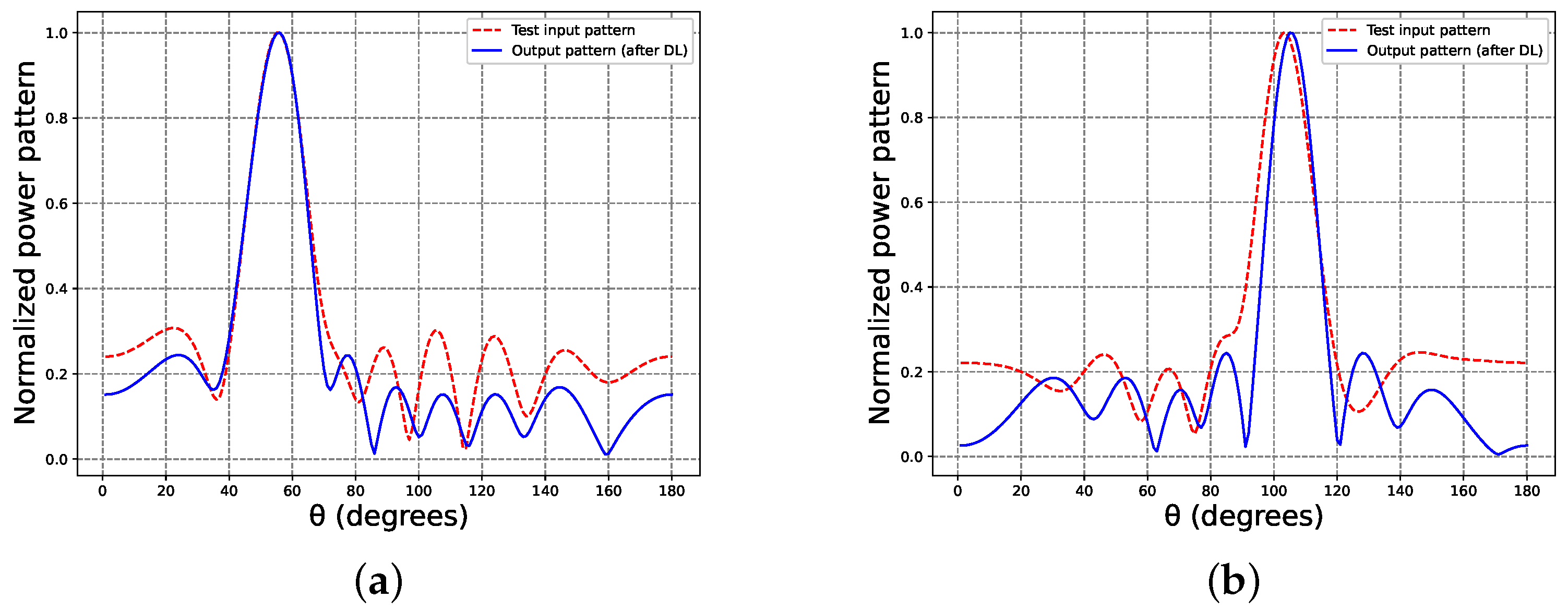
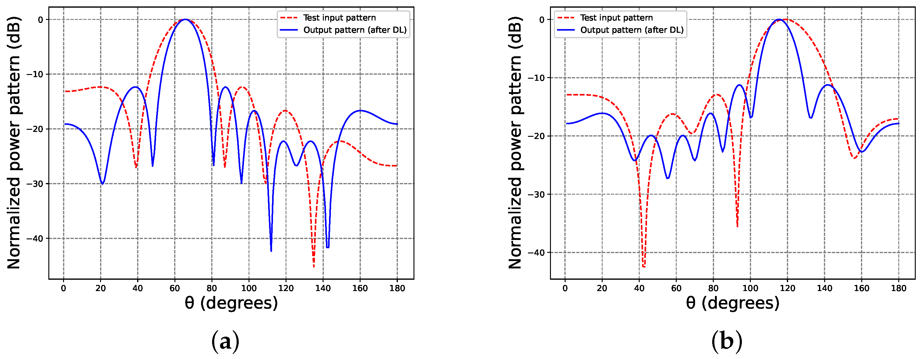
As part of a test case, we synthesized radiation patterns at fixed locations where the test data do not overlap with the training data; in other words, with radiation patterns that the neural networks had never seen before. Specifically, the deep neural networks (DNNs) had not been trained using these specific positions. Figure 6 illustrates the test input patterns at 55° and 105° (shown as dashed lines). Additionally, the recurrent neural network (RNN) provided predictions for these inputs, represented by the synthesized patterns (continuous lines) at these locations. It is essential to mention that radiation patterns of the training data were generated within the range of $50°\le \theta \le 130°$, with the phase incremented by 20°, completely differing from the validation and test data. Furthermore, Table 2 displays the complex excitation produced by the RNN for these test patterns.

The final radiation synthesis result highlights the DNN’s capability to effectively manage the trade-off between antenna parameters (SLL and D), thanks to the information learned during the pre-synthesis process of the beam patterns. Moreover, the proposed DNN demonstrated the ability to predict and adapt to any direction of interest, including ideal beam shapes, as illustrated in Figure 5. Specific numerical values for the sidelobe level and directivity of the output patterns generated by the RNN (both ideal and test patterns) are presented in

Table 3. Sidelobe level and directivity (output data) of the LSTM-RNN.

Triangular Pattern		Square Pattern		Test Pattern 1		Test Pattern 2
SLL (dB)	$\mathit{D}$ (dB)	SLL (dB)	$\mathit{D}$ (dB)	SLL (dB)	$\mathit{D}$ (dB)	SLL (dB)	$\mathit{D}$ (dB)
−11.83	8.10	−12.15	7.81	−12.25	7.60	−12.24	8.58

. On average, the output beam patterns achieved an isolation level of approximately 12 dB and a directivity close to 8 dB. These results, produced by the LSTM-RNN, are closely aligned with the near-optimal outcomes (based on their fitness and according to the case study) obtained with the metaheuristic optimizer used in the training phase.

Interactions Between Array Elements

To analyze the capabilities of the proposed approach (LMST-RNN), a scenario involving strong interactions between array antenna elements was considered. The analysis, based on the array factor, modeled the geometric and phase interaction between the array elements without considering the specific electromagnetic details of each radiator. This approach provides an initial approximation of how the array elements affect the radiation pattern due to their separation and relative phase. The effects of recurrent deep learning were analyzed with the antenna elements separated by only 0.3$\lambda$ (where the typical distance is 0.5$\lambda$). By applying the same methodology used previously but changing the distance between elements to 0.3$\lambda$, the results represented in Figure 7 were obtained.

From Figure 7, we can clearly observe the effects of the interaction between array elements on the beam pattern in both cases, directly impacting the visible characteristics of the radiation pattern, such as the beam width, through reducing directivity and causing issues related to beam steering despite the pre-conditioning phase. On the other hand, in general, we can observe a significant improvement in the output of the network in both cases, making the beam more directive and adjusting the beam steering. Specifically, in Figure 7a, a beam pattern at 65° with geometric and phase coupling interference is shown as input to the network, with an isolation level of $-12.3$ dB and a directivity of $6.25$ dB. At the network’s output, a better performance was achieved, with a directivity of $8.33$ dB and an SLL of $-12.3$ dB. In the case of Figure 7b, there was a similar behavior at 115° with an SLL value of $-12.9$ dB and only $5.9$ dB in directivity. At the output, a sidelobe level of $-11.23$ dB and a directivity of $8.07$ dB were achieved in the beam pattern. It is worth highlighting that geometric and phase coupling is a significant concern in applications where antennas are arranged in close proximity, such as in beamforming arrays, MIMO systems, or satellite communications. In such cases, minimizing this phenomenon is essential to prevent signal quality degradation and to maintain optimal system performance.

3.4. Runtime Analysis

Runtime analysis is an essential part of evaluating algorithms and systems, as it provides insights into the actual time efficiency of a solution under practical conditions. In this analysis, we focused on the execution time of both the training and inference stages rather than theoretical time complexity, which refers to how the execution time scales with the size of the input n. For the beam pattern synthesis of uniform linear arrays, the LSTM network took 7.991 min for the training stage on average; however, this is not critical, as training is typically performed offline. On the other hand, the trained network required 0.072 s to process the 92 test patterns on average. This demonstrates that, once trained, the network can generate beam patterns efficiently in real-time scenarios.

4. Discussion

Conducting case study analyses in terms of the array factor has the advantage of generalizability, allowing the obtained findings to be efficiently and straightforwardly translated to various applications in different areas without the need to be tied to a specific antenna type or application.

Deep hidden layers were used in ANNs to provide antenna design parameters for arbitrary beam patterns, which previously may not have been possible. Due to this characteristic in antenna radiation patterns, the proposed network could be used to solve practical antenna problems, such as those related to beamforming and coupling, among others. It is worth noting, furthermore, that the development of DNNs that are capable of generating adaptive beamforming, such as the proposed RNN in this work, makes them suitable for use in dynamic applications, where quasi-optimal solutions may become the better option.

Improving the beam pattern beforehand through a metaheuristic algorithm helped us enhance the antenna parameters, specifically, the SLL and D. This ultimately translates into a DNN, which is capable of solving interference mitigation and pointing problems. Furthermore, the combined use of EAs with DL allowed us to significantly reduce the computational burden by eliminating the need to simulate a specific result for each possible beam position.

In the same vein, data pre-conditioning based on the isolation level and directivity allowed us to utilize quality metrics that are even more meaningful for antenna designers. However, the network was not directly trained with these metrics, mainly because they are not differentiable with respect to the input parameters, and this issue has been previously mentioned by some authors [23]. However, it is worth noting, as this behavior is also observed in our analysis, where we used the MSE as the loss function, thus aiding the RNN in generating similar beam patterns to those it was trained with.

Another notable aspect is that, unlike MLPs, CNNs and LSTMs are neural networks that have been widely employed for time-series analysis. CNNs excel at capturing the relationships among various data points within each time series, allowing them to provide accurate predictions. On the other hand, LSTMs are particularly effective at capturing temporal and sequential relationships in the input data due to their ability to retain past inputs. This capability is crucial for analyzing radiation patterns, as it involves understanding the evolution of patterns over time and modeling long-term dependencies among the input data. Therefore, LSTMs are a favorable choice for beam pattern synthesis, as they can effectively learn and adequately represent the changing complexity of radiation patterns in the antenna array.

Finally, before achieving the results shown in Table 1, we trained the proposed architectures with fewer training patterns (e.g., 2264 training patterns), and error levels of magnitude ten times higher were obtained. To solve this problem, we added more training patterns and performed tuning in the neural architectures until we finished with the presented results. This occurred as deep learning essentially involves curve fitting and, for a model to achieve high performance, it must be trained on a comprehensive and dense representation of its input space. In this context, “dense sampling” means that the training data should thoroughly encompass the entire manifold of the input data, particularly around the decision boundaries. When the sampling is sufficiently dense, the model can interpret new inputs by interpolating between previously seen training examples [31]. Otherwise, although deep learning approaches have achieved outstanding results in almost all areas of knowledge, deep algorithms still require a large amount of data to achieve good performance [32,33,34].

5. Conclusions

A methodology based on deep learning using an RNN was introduced and developed for the synthesis of beam patterns for linear arrays. A comparative study among three well-known DNN architectures showed that the LSTM-RNN architecture exhibited better prediction performance in terms of the MAE and MSE. Additionally, the proposed RNN, which was trained and validated on 7623 and 32 previously optimized radiation pattern samples, respectively, demonstrated satisfactory performance in synthesizing corresponding beam patterns with low sidelobe levels and enhanced directivity. The test results of the LSMT-RNN validate that DL is viable for synthesizing ideal radiation patterns (which are characterized by high prediction complexity) and attainable radiation patterns, including geometric and phase coupling effects. In most cases, the outputs closely resembled the input beam patterns, demonstrating the reliability of the approach for beam pattern synthesis within a certain range of input configurations and their potential for application in point-to-point wireless communications, broadcasting, and radar systems, among others. Future research will explore the potential of the RNN-based methodology to complete antenna systems, including beamforming networks. This would involve developing techniques to seamlessly interface the DNN with beamforming hardware, allowing for real-time (or near real-time) adaptation and optimization of beam patterns depending on changing environmental conditions, signal requirements, or system objectives. Further studies will also investigate the feasibility of applying the proposed RNN under various antenna array geometries with different configurations beyond linear arrays. This could involve adapting the model architecture and training process to accommodate different antenna geometries, configurations, and design parameters, as could be the case in two-dimensional synthesis. Finally, although the LSTM-RNN architecture obtained promising results, exploring alternative deep learning architectures and methodologies could provide further insights and improvements in the context of antenna synthesis. This would entail investigating other variants of recurrent neural networks or exploring the use of hybrid architectures.