1. Introduction
The vigorous development of satellite communication meets the needs of social development. In recent years, with the rise of low earth orbit constellations, the demand for data exchange between satellites is increasing, thus there is a great demand for spectrum resources. The L, S, C, X, Ku, and Ka frequency bands for traditional satellite communication are very scarce. As an undeveloped band of the electromagnetic spectrum, the terahertz band has a frequency between 0.1~10 THz, which has a high spectrum bandwidth to realize high-speed data transmission, and has great application value in satellite communication. At present, International Telecommunication Union has completed the frequency division of satellite services in the frequency range of 100~275 GHz and has made a simple division of the terahertz frequency band above 275 GHz. At the same time, the development of terahertz devices is progressing steadily. The terahertz frequency band has been preliminarily qualified for application in satellite communication.
The modeling of inter-satellite terahertz channel is the basis for realizing the application of inter-satellite terahertz wireless communication. The channel through which terahertz waves are transmitted from the transmitter antenna to the receiver antenna is the terahertz wireless channel, and the characteristics of the channel determine the performance of satellite communication systems. The terahertz channel model is the foundation for the design and optimization of terahertz communication systems. Channel modeling is based on data measured by existing channel measurement platforms, using mathematical formulas to characterize various parameters of the channel.
There have been many researches on the modeling of terahertz channel in terrestrial communication [
1,
2,
3,
4]. Tian et al. [
1] provided a detailed explanation of the characteristics of ground terahertz channels. The terahertz frequency is large and the wavelength is short, so the terahertz channel has different channel characteristics compared with the low-frequency channel. As terahertz travels through the atmosphere, molecules such as water vapor, clouds, ice crystals, and dust increase path losses. Han et al. [
2] analyzed the existing terahertz channel models and introduced channel simulators based on these models. Including NYUSIM, Cloud RT, EDX Advanced Promotion, etc. These models are mainly applied in ground communication scenarios such as indoor offices and outdoor environments.
However, to our knowledge, there is currently a lack of research on channel modeling for inter-satellite terahertz communications, therefore it is necessary to conduct relevant research.
In addition, in terms of channel modeling methods, channel modeling methods include deterministic modeling and statistical modeling. The deterministic channel modeling method is based on the analysis of optical and electromagnetic propagation theories in current application scenarios to establish a wireless channel model. Priebe et al. [
5] used ray tracing technology to model a 300 GHz indoor environment and used a free space path loss formula to model large-scale fading of line-of-sight links. For small-scale fading, the line-of-sight links delay is modeled as
, recursively calculating the delay of each order of reflection path. The line-of-sight links phase is modeled as the first-order function of the delay
, the phase on the reflection path is uniformly modeled within −180° and 180°. And model the horizontal angle of arrival (AOA) uniformly, and calculate the horizontal angle of departure (AOD) by adding a difference value on the AOA, which is equal to a multiple of 180°. The advantage of the deterministic channel modeling method is that it does not require actual measurement, but its disadvantage is that it requires very detailed application scenario information and high computational complexity. Sometimes, in order to make the modeled channel model more concise and practical, deterministic channel modeling methods may have certain trade-offs and idealization of the parameters that affect the channel during modeling. Therefore, some scholars use statistical modeling methods for channel modeling.
Statistical channel modeling uses a measurement platform to measure channel data in actual application scenarios and fits the actual data to obtain the empirical distribution and statistical characteristics of each channel parameter. Finally, the channel is reconstructed based on statistical characteristics.
He et al. [
6] conducted channel measurements from 220 GHz to 340 GHz using a vector network analyzer and proposed a propagation channel model for the terahertz band. It is represented by a logarithmic model:
According to the measurement results, it was found .
Traditional statistical methods rely on manually constructing mathematical channel model from data, which is time-consuming. In order to solve this problem, some researchers use neural networks to directly fit the channel model. On the one hand, for the existing wireless channel models, it is only necessary to train the neural network with the data generated by the corresponding models, so that the neural network can approximate the actual channel model under the minimum mean square error criterion. On the other hand, for wireless channels without channel models, neural network-based channel modeling uses measured data for training and does not need to determine the propagation path of electromagnetic waves, so it is not constrained by the environment and is more suitable for various complex scenarios. When the actual wireless channels are nonlinear/non-stationary, neural networks have a good performance in simulating nonlinear systems. Neural networks can train high-dimensional nonlinear data, and solve many problems that are difficult to be solved by traditional modeling methods.
Bai et al. [
7] proposed a 3D MIMO indoor channel modeling method targeting the millimeter wave frequency band. Based on the convolutional neural network model, the input data are the coordinates of the transmitter and receiver, and the output characteristic parameters include the received power, delay, transmission azimuth, transmission elevation, arrival azimuth, and arrival elevation.
Ferreira et al. [
8] used neural networks to improve the prediction of outdoor signal strength in the ultra-high frequency (UHF) band. The diffraction loss and transmitted signal strength are fed into the neural network and the strength of the received signal will be output at the output layer. The results show that the neural networks can improve the prediction of outdoor signal strength in the UHF band.
However, these methods of using neural networks as a channel model make it difficult to reveal the mathematical characteristics and physical mechanism of the channel because of the interpretability issue of neural networks.
Xue et al. [
9] noted the interpretability issue of using neural networks as a channel model and proposed a scheme to use causal neural networks for channel modeling. However, this method still uses neural networks directly as the channel model, although it enhances the interpretability of neural networks, it is not intuitive enough. In order to solve the problem of insufficient interpretability of neural network channels, Lee et al. [
10] first used channel data to train the neural networks as a channel model, and then used a genetic algorithm to generate a symbolic regression formula from the neural network channel model. This is the indirect use of the symbolic regression method to generate the channel model. This indirection may be unnecessary.
Given the analysis of the above factors, this paper proposes a transformer symbolic regression-based inter-satellite terahertz channel modeling method which is based on the symbolic regression method PhySO [
11]. It uses a transformer neural network as a tool to directly fit the mathematical channel model from the measured channel data, avoiding the laborious problem of establishing a mathematical channel model by traditional statistical methods and the interpretability issue caused by using a neural network as a channel model, and can reveal the mathematical relationship and physical mechanism between channel parameters.
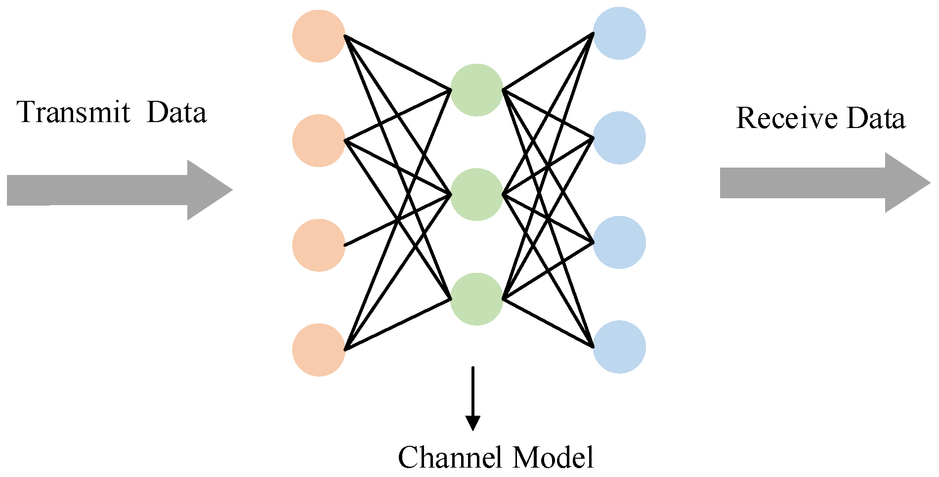
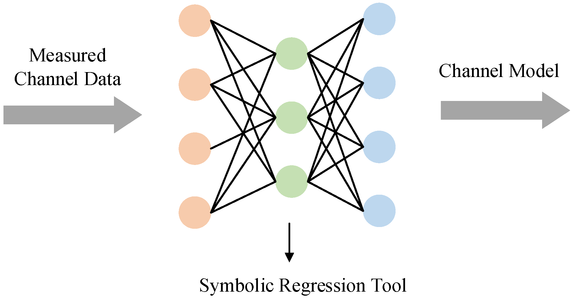
Figure 1 and
Figure 2 show the difference between using neural networks directly as channel model and using deep neural network as a symbolic regression tool to generate channel model.
The main contribution of this paper are:
To the best of our knowledge, it is the first time to establish a mathematical channel model directly from data by using a symbolic regression method. As a new channel modeling method, it may help researchers to establish a channel model easily.
The PhySO method is improved to be more suitable for channel modeling tasks.
The method proposed in this article may have important application prospects in the field of channel modeling. Although this article takes the terahertz frequency band as an example, it has a wide range of applications and can be used as a data-fitting tool for other frequency bands and more complex communication scenarios.
This paper is organized as follows:
Section 1, introduces the important role of channel modeling in the future inter-satellite terahertz communication systems, expounds on the shortcomings of the traditional channel modeling scheme and the use of neural network as the channel model scheme, and proposes a channel modeling scheme based on symbolic regression.
Section 2, introduces the symbolic regression method, especially the PhySO symbolic regression method in detail, and the corresponding improvement to PhySO, which makes it more suitable for the channel modeling task.
Section 3, simulates the fitting effect of the improved PhySO symbolic regression method on the free space path loss model and verifies the feasibility of the proposed method. In
Section 4, it summarizes the characteristics of the proposed method and points out the next research plan.
2. Transformer Symbolic Regression
2.1. Symbolic Regression
Symbolic regression is a technique aimed to automatically discover mathematical expressions or functions from data sets [
12].
Set target dataset and label , symbolic regression aims to find a function so that where indicates the evaluation of formula . For example, .
Symbolic regression is considered an extension of traditional regression methods, traditional regression methods need to assume that the data follows a polynomial distribution or some other distribution while symbolic regression doesn’t have to. Symbolic regression can automatically discover nonlinear and higher-order relationships in the data, and can also be applied to multivariable problems to discover interactions between multiple variables. It can be used to uncover underlying patterns behind data to help researchers find real models and mechanisms.
Symbolic regression is mainly realized by genetic algorithm and deep reinforcement learning algorithm.
Traditional symbolic regression algorithms mainly use genetic algorithms to search for feasible mathematical expressions.
The specific steps of using the genetic algorithms to search for the optimal formula are as follows:
Set the initial space of arithmetic variables, operations and end conditions during the running process;
Initial formula set as population;
Evaluate the formulas based on evaluation such as the mean square error between the predicted values of formulas and the data labels;
Generate a new population by replication, crossover, and mutation operations;
Repeat steps 3 and 4 until the end condition is met, and sort the generated formula set based on the evaluations to choose the best formula.
Symbolic regression based on genetic algorithm has some problems, it cannot take advantage of the inherent characteristics of the dataset to search for suitable formula, so the search process will be too long, the search is too inefficient, and it is easy to fall into local optimal.
In recent years, deep reinforcement learning has made great progress in the field of optimization solutions. Many studies have applied deep reinforcement learning to solve symbolic regression problems. This kind of method can search symbols from the symbol space (the space of variables and operations), construct a mathematical expression from the symbols, and get a reward according to the fitness of the mathematical expression to optimize the strategy function. Deep reinforcement learning can achieve very good results in symbolic regression problems [
13].
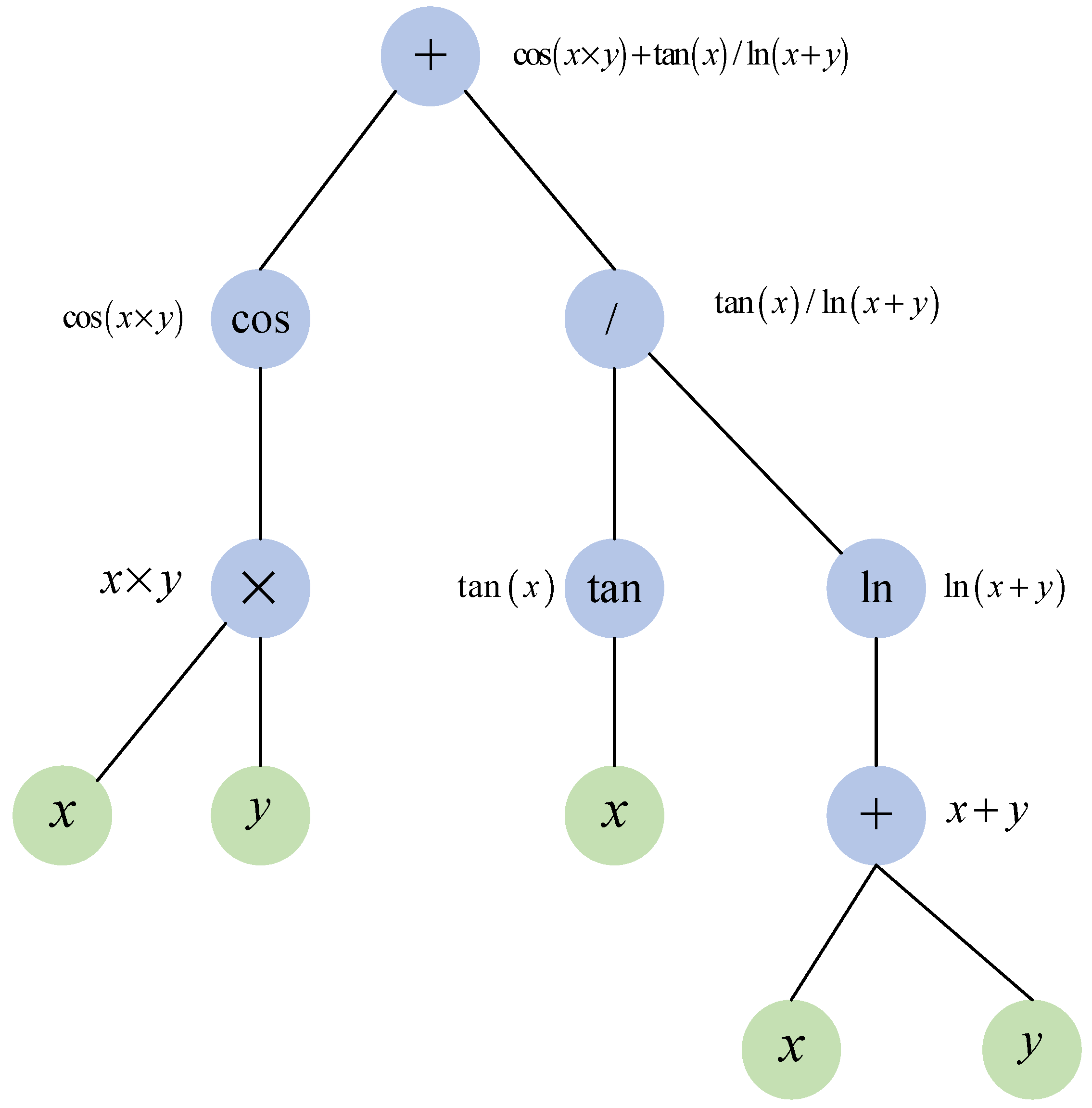
Deep learning-based symbolic regression methods often model formulas as binary trees, the nodes of the tree are called symbols which are divided into variables in green and operations in blue of mathematical, as shown in
Figure 3, the binary tree can be converted into mathematical formulas by depth-first search of mid-order traversal, and it is
. Therefore, the problem of symbolic space exploration is regarded as the generation problem of a formula binary tree.
2.2. PhySO
Thanks to Tenachi et al., they proposed PhySO [
11], a powerful deep reinforcement learning-based symbolic regression method. It builds a mathematical expression starting from the most basic physical units and automatically detects and corrects combinations of symbols that may lead to violations of physical unit constraints, ensuring that unit correctness is maintained throughout all computations. This avoids generating irrational mathematical expressions and greatly reduces the size of the expression search space, so the search process of PhySO is more efficient and can find the best solution faster.
In the implementation, PhySO models mathematical expressions as binary trees, where variables and coefficients are terminal nodes, operation symbols are non-terminal nodes, monadic operators have only 1 child node, and binocular operators have 2 child nodes. Variables and operators are called tokens in PhySO, and the space they make up is called Library, for example, Library = {a, b, c, +, −, /}. Tokens in the Library such as “a, b, c, +, −, /” are encoded by one-hot for subsequent processing by the neural network.
As a deep reinforcement learning method, PhySO sets the observations as parent nodes and their units, sibling nodes and their units, previous node and its unit, dangling nodes and the unit of the current node, and the initial observations are all zero tensor. The action is to select the tokens in the Library to build the mathematical expression. By prioritizing the output of the action by the neural network and performing the mask operation, it masks out unnecessary actions to generate better mathematical expressions. The reward is:
where
is the reward,
is the standard deviation of the target value,
is the number of sampling points,
is Bessel’s correction and
,
are data points and target values, and
is the function generated by the neural network.
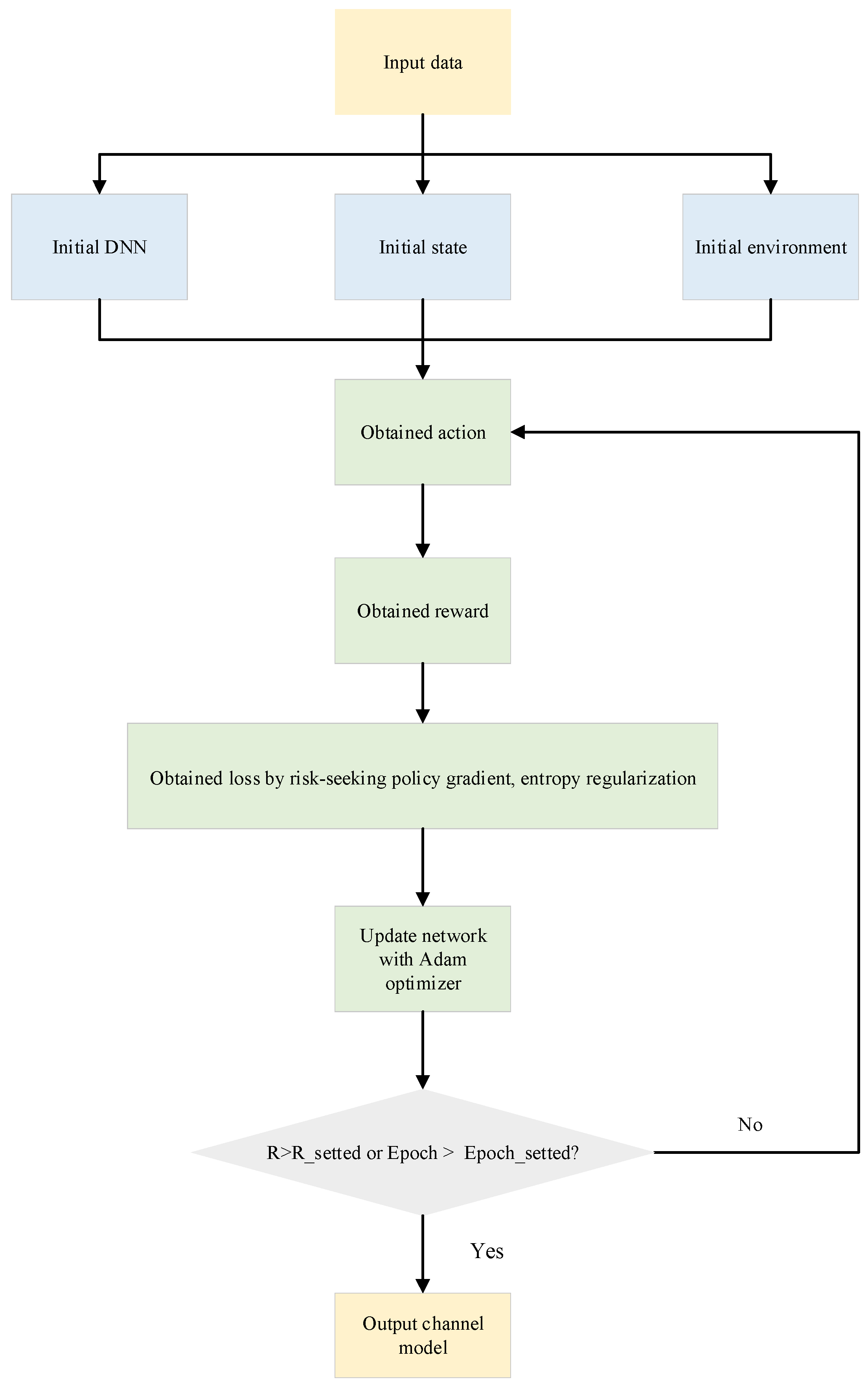
The optimization strategy used by PhySO is risk-seeking policy gradient [
14], entropy regularization [
15], and Adam optimizer is adopted. When the reward is big enough and the expression is meaningful, the algorithm will stop iterating and output the corresponding result.
The network architecture used by PhySO is Long Short-Term Memory (LSTM) which is a classical neural network architecture for processing sequence data. After the observations data is input into the LSTM network, the network will output the probability distribution of each action, adjust the probability distribution of the action by masking the actions that do not meet the constraint conditions, and then sample the action according to the probability. Then, based on the action, the new mathematical expression is obtained, and the observations are updated. It will be repeated until the final mathematical expression is obtained.
By deep reinforcement learning technology, the PhySO method can adaptively adjust learning strategies, and automatically select the most appropriate mathematical expression to describe data by using physical constraints and avoid meaningless symbol combinations. This method can greatly improve the search efficiency and reliability of the model, and can better adapt to different types of physical data.
2.3. Improved PhySO Algorithm
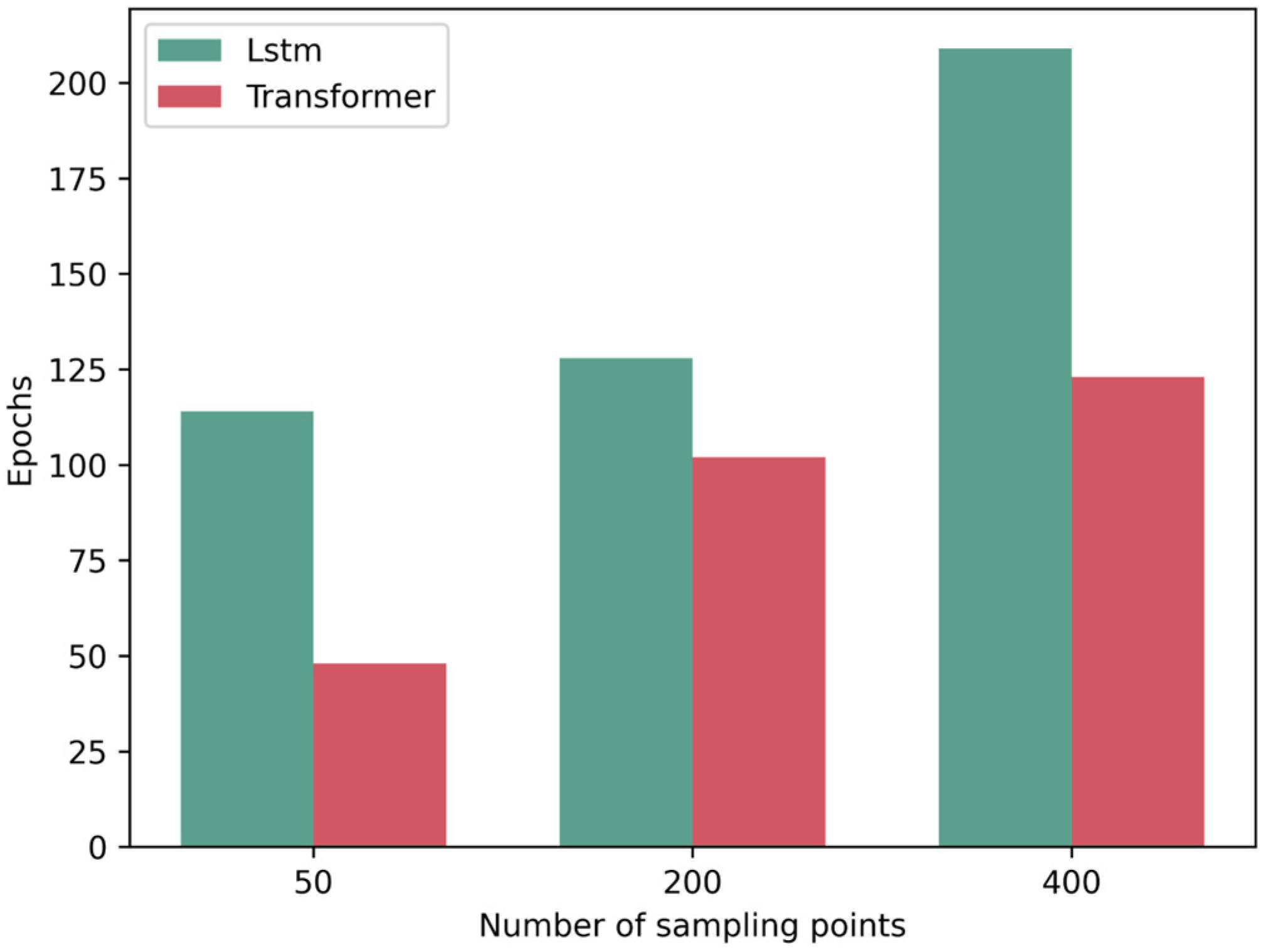
In the PhySO project, the authors used LSTM as a neural network architecture, and only the optimal 5% of candidate solutions were rewarded. However, LSTM has the problem of poor parallel performance, and each LSTM cell has four fully connected layers, if the LSTM network is very deep, the computational load will be large and time-consuming. And only the optimal 5% candidate solution is rewarded, when the channel mathematical model is relatively complex, such as when there are mixed operations of logarithm, exponent, fraction, and trigonometric function in mathematical expressions, there are problems of poor exploration performance and slow convergence. In addition, in the process of generating a channel model with PhySO, multilayer fractions, and multilayer exponents often appear, which are not common in the channel model. In order to solve these problems, the PhySO method is improved to make it more suitable for channel modeling tasks.
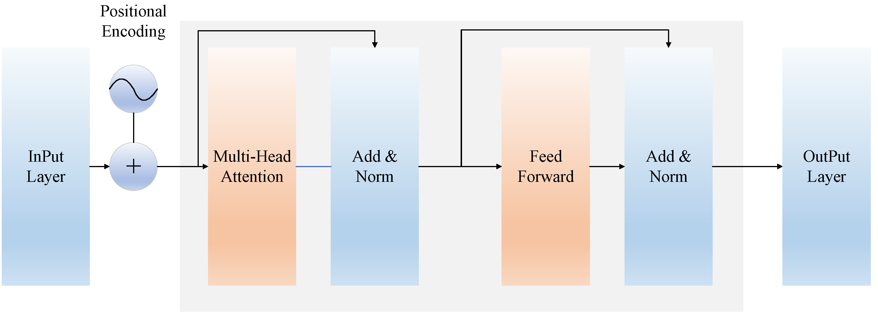
In this paper, the LSTM architecture is changed to transformer architecture [
16] to increase the parallel performance and feature extraction capability of the algorithm. The self-attention mechanism in the transformer architecture enables the calculation of each time step to only rely on the input vector, thus achieving completely parallel computation. Moreover, the self-attention mechanism can directly calculate the dependency relationship between any two positions in the sequence, making the model better able to capture long-distance dependencies. The structure of the transformer model is very flexible and can be adjusted according to the needs of specific tasks, such as increasing or decreasing the number of layers and adjusting the number of attention mechanism heads. Its architecture diagram, as shown in
Figure 4, includes the input layer, transformer layer, and output layer. Both the input and output layers are linear layers, and the transformer architecture used contains only the Encoder part, which is used to extract the features of mathematical expressions.
In the process of exploration, the optimal 5% candidate solution is changed to the optimal candidate solution decreasing from 10–5% to increase the exploration effect of the model.
According to the channel model expression, the symbol space is redefined as . By reducing unnecessary operators, search complexity can be reduced and convergence speed can be accelerated.
Modify the config file of the PhySO project to reduce the occurrence probability of multiple fractions and exponents. Because in the common channel model, it is unusual to see the nested fraction and exponential function. By reducing the nesting of fractional, exponential, and logarithmic operations, the complexity of algorithm search can also be reduced, resulting in a faster search for the optimal expression.
The logarithmic function used in the PhySO project is changed to the logarithmic form with base 10, which is more consistent with the dB definition in the channel model.

