Article

Calibration Method of PFC3D Micro-Parameters under Impact Load

1
College of Pipeline and Civil Engineering, China University of Petroleum (East China), Qingdao 266580, China
2
College of Civil Engineering and Architecture, Shandong University of Science and Technology, Qingdao 266590, China
*
Author to whom correspondence should be addressed.
Appl. Sci. 2024, 14(7), 3020; https://doi.org/10.3390/app14073020
Submission received: 7 March 2024 / Revised: 27 March 2024 / Accepted: 2 April 2024 / Published: 3 April 2024
(This article belongs to the Section Civil Engineering)

Abstract

:
Micro-parameter calibration is essential in constructing an accurate and reliable numerical model of particle discrete element PFC3D 6.0 software. Micro-parameter calibration is mainly accomplished according to the macro-parameters obtained from static or quasi-static laboratory tests such as UCS. However, there is little current research concerning the calibration method under impact load. An SJM micro-parameter calibration method, based on the SHPB rock test and the FLAC3D/PFC3D coupling method, is proposed to solve this problem. Firstly, UCS, SHPB, and other laboratory rock tests were carried out to determine the rock sample’s macroscopic physical and mechanical parameters. Secondly, the FLAC3D/PFC3D numerical coupling model of the SHPB test was established, and the single-factor and double-factor orthogonal numerical simulation was carried out. Then, the main micro-parameters that affect the macroscopic physical and mechanical parameters of the SJM particle discrete element model were proposed. Finally, the quantitative relationship between the model’s macro-parameters and micro-parameters was established through multiple linear regression. A set of PFC3D micro-parameter calibration processes under impact load was established. The relative errors of the macro-parameters obtained from laboratory and numerical tests totaled less than 5%, which further verifies the rationality of the calibration method. This method provides some reference values for PFC3D micro-parameter calibration under impact load.

1. Introduction

Particle discrete element PFC3D software uses many contacting particles to describe the mechanical properties of real material media. This description differs from the existing testing and specification methods. It is difficult to directly obtain the particles’ micro-parameters. Therefore, it is necessary to calibrate the micro-mechanical parameters, such as particle and contact properties, through three typical numerical rock mechanics tests: triaxial compression, Brazilian splitting, and tensile testing.
Castro-Filgueira et al. evaluated the influence of the micro-mechanical parameters of the PFC model on its macro-mechanical parameters through sensitivity analysis [1]. Xu et al. proposed a new linear parallel bond model (CM-LPBM) calibration method for the PFC micro-mechanical parameters [2]. Li et al. established the calculation formulas for the microscopic and macroscopic parameters of rock materials through regression analysis and quantitatively analyzed the micro-parameters of PFC3D [3]. Ajamzadeh et al. studied the influence of PFC micro-parameters on UCS and Brazilian splitting test results [4]. Xu et al. proposed a set of standardized micro-parameter calibration procedures for LPBM and the smooth joint model (SJM) [5]. Su et al. used MATLAB and a genetic algorithm to write the micro-parameter calibration program of the concrete model and the inversion of its macro-parameters [6]. Shi et al. used the cellular automata method to establish a discrete element model of clustered particles and proposed a fast and effective calibration method for rock micro-parameters [7]. Yoon estimated the nonlinear relationship between the microscopic and macroscopic parameters of the PFC model using the statistical center composite design (CCD) method [8]. Wu et al. proposed an optimization method combining Box–Behnken experimental design and expectation function to quickly calibrate micro-parameters [9]. Zou et al. proposed a combinatorial optimization method (GT-RSM-MD) to effectively calibrate micro-parameters [10]. In addition to the PFC software, other discrete element methods also need to calibrate micro-parameters. Tatone et al. developed the y-Geo FDEM code to obtain the model parameters for the bonded-particle DEM and FDEM method [11]. Cheng et al. proposed a calibration method to calibrate DEM parameters, considering the coupling effect of micro-parameters [12].
However, the microscopic parameters calibrated using static mechanical properties of rocks are often unsuitable for high strain-rate numerical tests. Therefore, this problem must be solved according to the dynamic mechanical properties of rock. The primary test method used to obtain the dynamic mechanical properties of rock is the split Hopkinson pressure bar test (SHPB). The SHPB test has been used to study the dynamic mechanical properties of rock. Zhao et al. used the SHPB test to conduct the dynamic indirect tensile test on coal samples. They studied the influence of the bedding structure in coal seams on their dynamic indirect tensile strength [13]. Ai et al. used the SHPB system to study the dynamic mechanical properties of horizontal and vertical bedding coal samples [14]. Kong et al. used SHPB to conduct dynamic impact tests on gas-bearing coal [15]. In addition, many scholars have used the SHPB test to study materials such as coal, granite, limestone, marble, and concrete [16,17,18,19,20,21]. Qiu et al. used SHPB to carry out impact compression tests on laminated sandstone with different bedding inclination angles and used a high-speed camera to capture the fracture process of samples [22]. Wang et al. used the SHPB device to conduct cyclic impact tests on soil with different axial compression and impact velocities [23]. Yang et al. used the SHPB test to study the strength and microstructure of coal samples under an impact compression load [24].
Therefore, based on the SHPB rock test and the FLAC3D/PFC3D coupling method, a new calibration method for the SJM model of particle discrete element PFC3D software is proposed. Firstly, according to the in situ rock samples, the parallel bond model (PBM) and smooth joint model (SJM) in PFC3D were used to construct numerical specimens with bedded surfaces. The linear elastic model of FLAC3D was used to construct the incident bar and transmission bar of the SHPB experimental device. The bridging domain method was used to conduct the impact load between the PFC particles and the FLAC element. Then, several micro-parameters of SJM affecting the macro-mechanical parameters were determined using single-factor and double-factor orthogonal SHPB numerical tests.
Furthermore, through multiple linear regression analysis, the quantitative relationship between the micro-parameters of SJM and the macro-parameters of the rock sample was obtained. A set of the calibration processes for the micro-parameters of SJM under impact load was determined. Finally, the reliability of the proposed calibration method was verified by comparing it with the macro-parameters obtained from laboratory tests. A more accurate and reliable calibration method is proposed to determine the micro-parameters of the SJM model under impact load.

2. Laboratory Rock Test

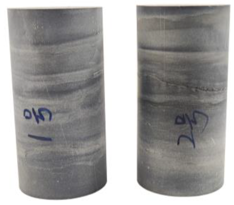
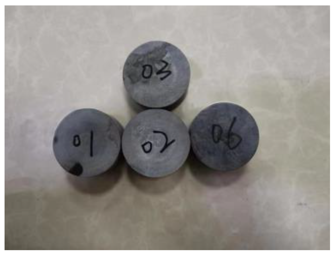
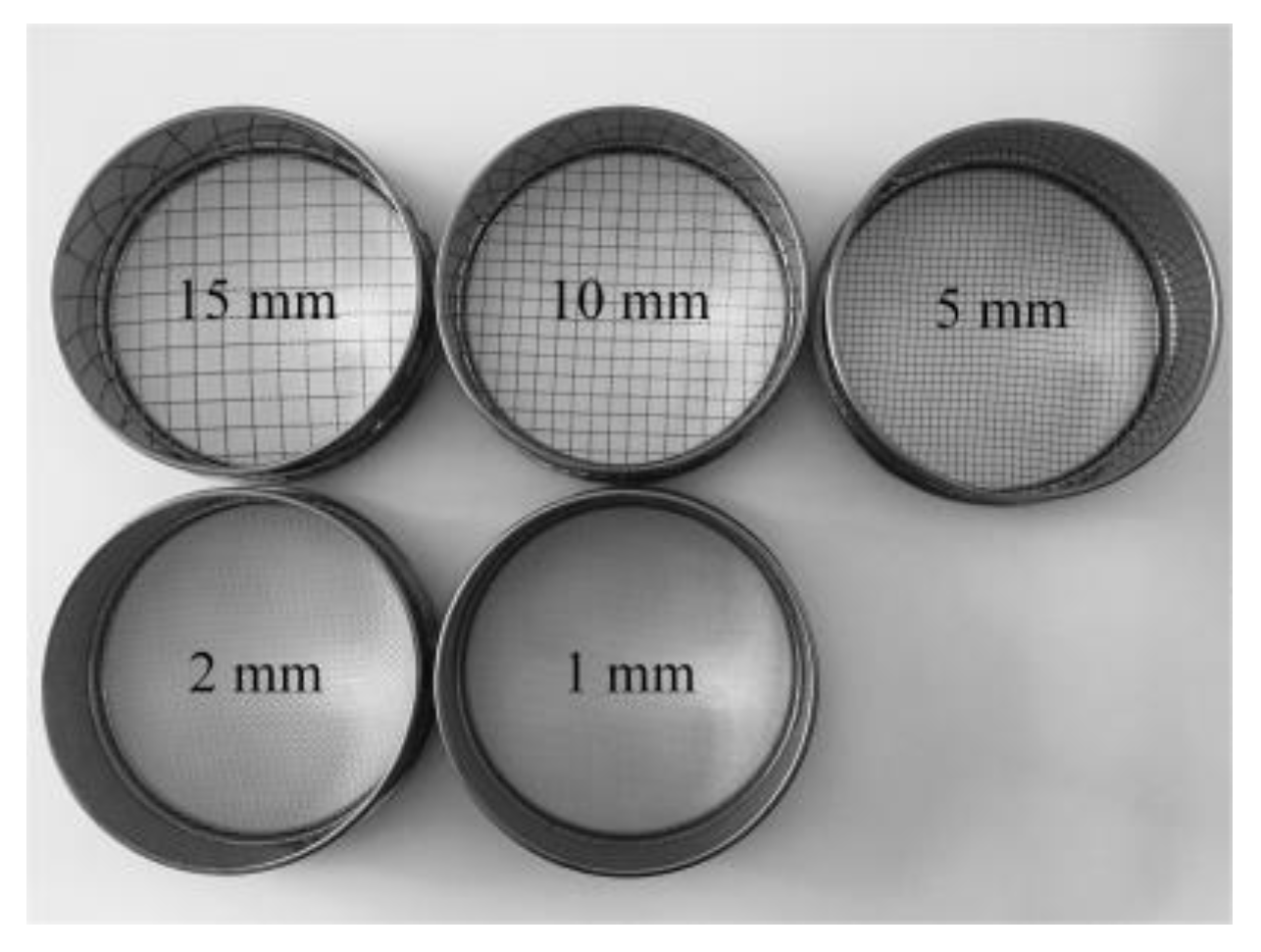
2.1. Rock Sample Preparation

Limestone with good integrity is selected from an open pit site. The samples required for the indoor rock test are created by core drilling, cutting, grinding, and other processes. For the UCS (Uniaxial compression specimen) sample, the size of the specimen is φ 50 mm × 100 mm, and the non-parallelism of the two end faces of the specimen is within 0.05 mm. The flatness of the end faces is within 0.02 mm. Some UCS specimens are shown in Figure 1.
In order to meet the one-dimensional stress wave propagation characteristics for the SHPB test and reduce the end friction and inertia effect, the slenderness ratio of the specimen is controlled at about 0.5. The size of the specimen is φ 50 mm × 25 mm, the non-parallelism of the two end faces of the specimen is within 0.05 mm, and the flatness of the end faces is within 0.02 mm. Some SHPB specimens are shown in Figure 2.

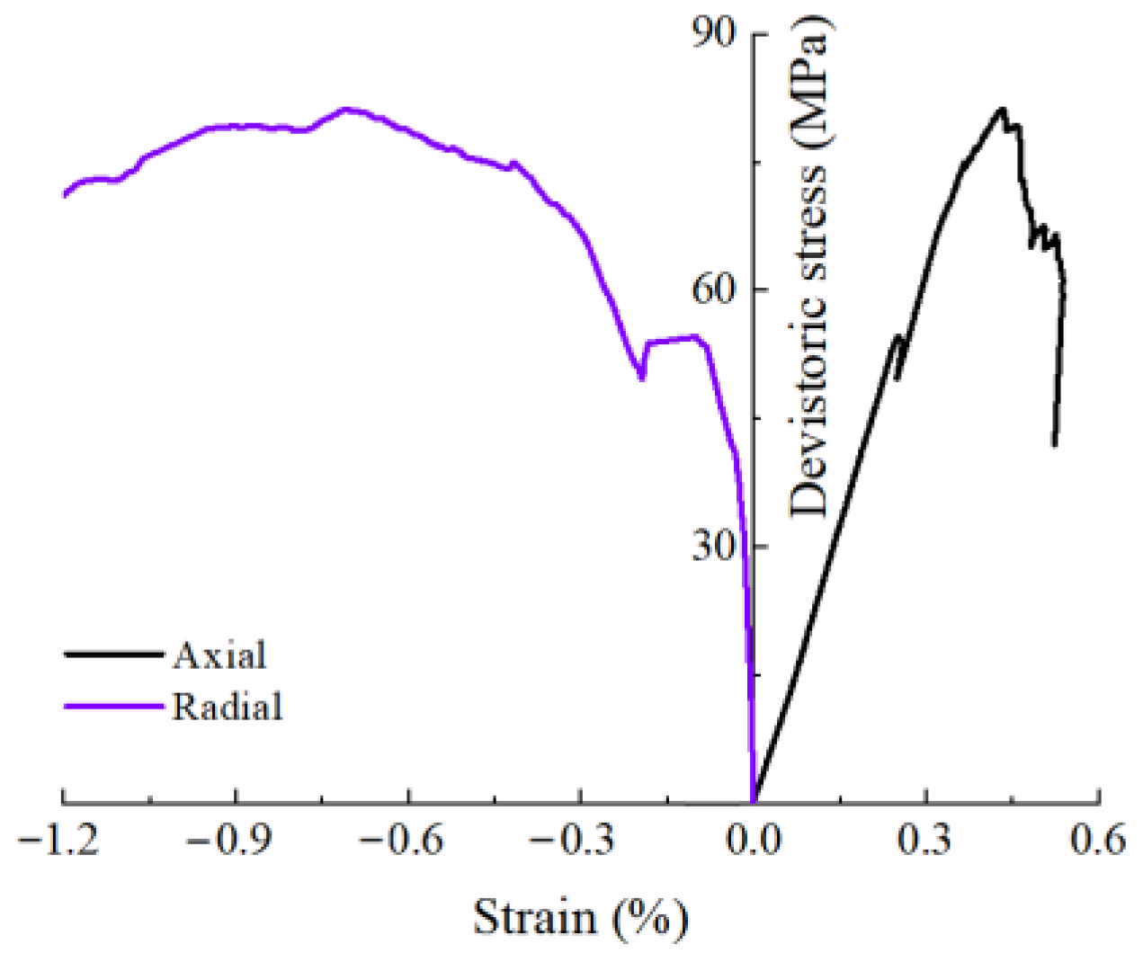
2.2. Static Physical and Mechanical Tests and Results

The basic physical properties of the rock samples, such as mass density and mineral composition, are essential parts of subsequent mechanical tests and micro-parameter calibration, so they are necessary in order to obtain the physical properties of the rock samples. The size and mass of the SHPB and UCS rock samples were determined, and the average density was 2.72 g/cm3. Then, three pieces of rock were randomly selected, ground to a particle size less than 40 μm, and placed in a drying box. A total of 0.2 g of dried limestone powder was used for X-ray diffraction analysis, performed using a Rigaku Ulima IV device. The diffraction angle was selected as 5°~80°, the tube voltage was 40 kV, the tube current was 40 mA, the test temperature was 25 °C, and the test humidity was 50%. The XRD test results are shown in Figure 3. The results of the quantitative composition measurement of limestone are shown in Table 1.
The TAW-1000 pressure servo testing system produced by Jilin Jinli Testing Technology Co., Ltd. (Jilin, China) can be used for uniaxial compression testing of limestone, as shown in Figure 4. The maximum axial test force during the test was 1000 kN. The axial displacement was 0.08 mm/min. The deviatoric stress–axial and radial strain curves obtained by the UCS are shown in Figure 5. The static peak strength of the limestone sample is 81.21 MPa. The elastic modulus is 22.69 GPa, and the Poisson’s ratio is 0.235.

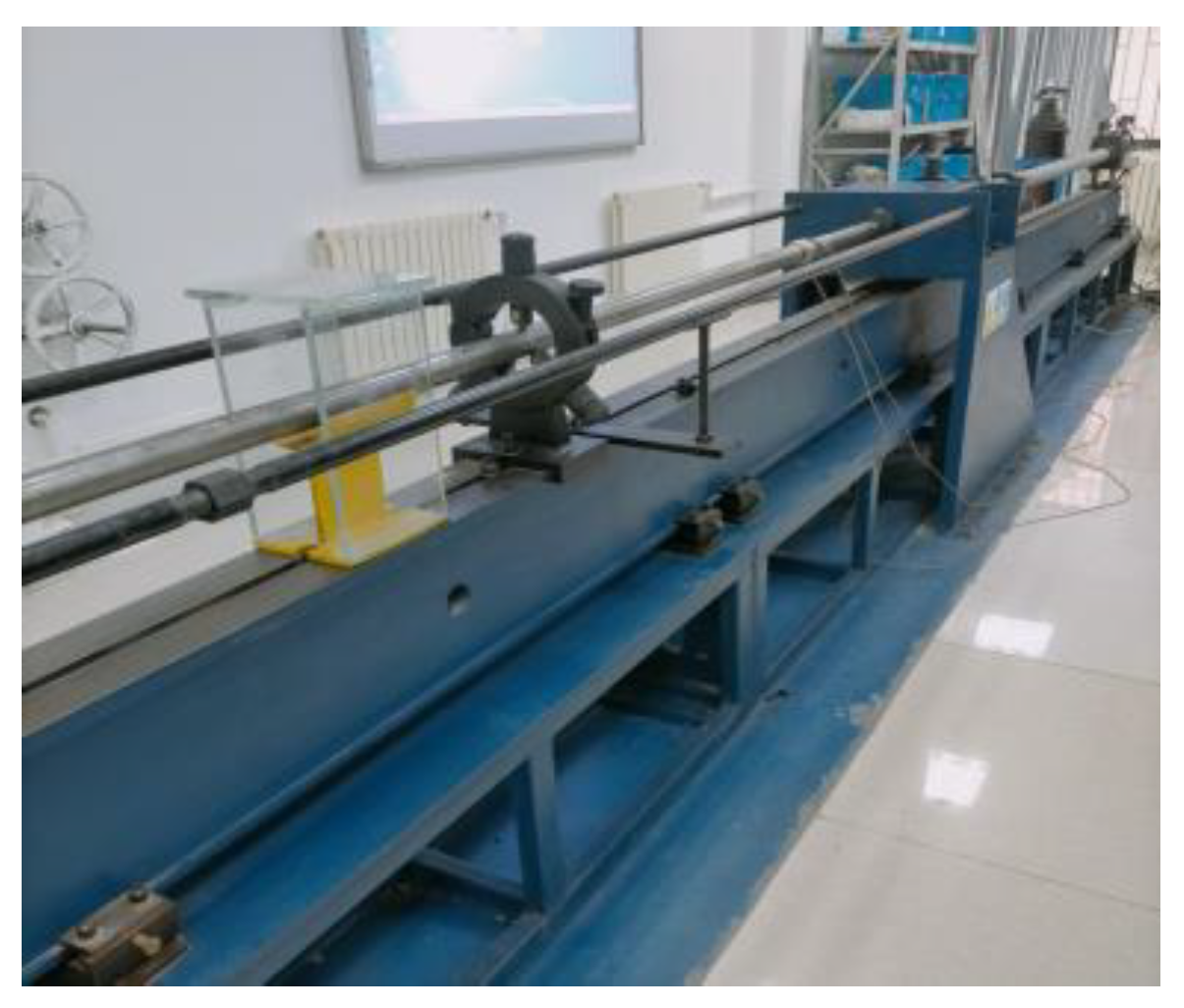
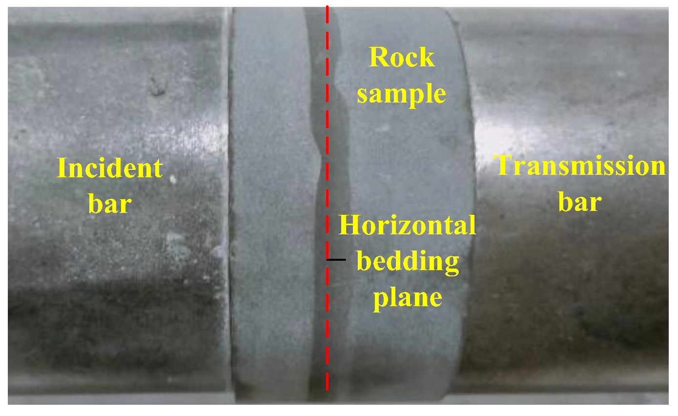
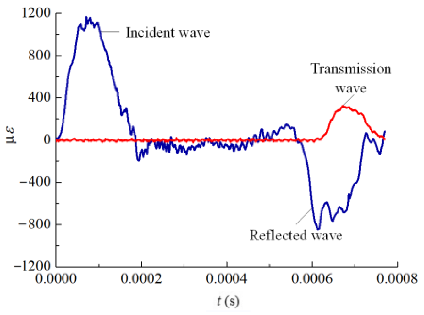
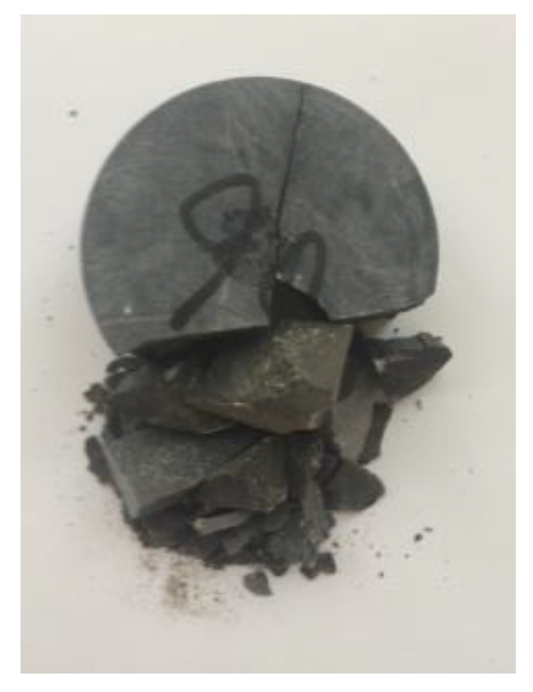
2.3. SHPB Test and Results

A uniaxial impact compression test was conducted on limestone samples using the SHPB testing system from Shaanxi Coal Chemical Group Co., Ltd. in Xi’an, China. The shock wave of the limestone samples was loaded at a driving pressure of 0.2 MPa. The test system and limestone samples in the clamping state are shown in Figure 6 and Figure 7.
The length of the absorption bar is 1.5 m, the length of the incident bar and transmission bar is 3.0 m, and the diameter is 50 mm. The bars are made of high-strength alloy steel, 48CrMoA, with a density of 7.8 g/cm3, an elastic modulus of 206 GPa, a yield strength of 835 MPa, and a P-wave velocity of 5172 m/s. The three-wave method was used to process the test data. In the SHPB test, incident energy Wi, transmitted energy Wt, and reflected energy Wr received by the specimen can be calculated as follows [25]:
W i t = A E C 0 0 t ε i 2 t d t
W r t = A E C 0 0 t ε r 2 t d t
W t t = A E C 0 0 t ε t 2 t d t
where A is the cross-sectional area of the bar, m2; E is the elastic modulus of the bar material; C0 is the longitudinal wave velocity of the bar, m/s; εi(t), εr(t), and εt(t) are the strain of the incident wave, reflected wave, and transmitted wave on the pressure bar at time, t respectively. Figure 8 shows the original waveform of three waves at the impact pressure of 0.2 MPa.
According to the one-dimensional stress wave theory and the assumption of uniformity introduced into the specimen, the average strain rate, average strain, and average stress on the two end faces of the specimen in the testing process are as follows [26]:
ε t = C 0 l s ε i t ε r t ε t t ε t = C 0 l s 0 t ε i t ε r t ε t t d t σ t = A E 2 A s ε i t + ε r t + ε t t
where l s and A s are the length and cross-sectional area of the rock specimen.
Figure 9 shows the deviatoric stress–strain curve when the impact pressure is 0.2 MPa, after calculation by the three-wave method. The dynamic peak strength and dynamic elastic modulus of the limestone sample are 84.29 MPa and 34.14 GPa, respectively.
The failure pattern of the limestone sample when the impact pressure is 0.2 MPa is shown in Figure 10. After impact damage occurred, the limestone samples were screened and weighed using a set of sizing screens and an electronic balance [27]. A set of sizing screens selected for the test is shown in Figure 11. The pore sizes, from small to large, are 1.0 mm, 2.0 mm, 5.0 mm, 10.0 mm, and 15.0 mm. Six groups of limestone fragments, with particle sizes ranging from 15.0~50.0 mm, 10.0~15.0 mm, 5.0~10.0 mm, 2.0~5.0 mm, 1.0~2.0 mm, and 0.0~1.0 mm, were obtained through screening, as shown in Figure 12. In order of particles sizes, the range obtained was i = 1, 2, 3…6. After the screening, the percentage of the mass of fragments in each group and the total mass of the sample was counted. The method of obtaining these results is as follows: firstly, a set of sizing screens was used to screen the broken fragments; secondly, an electronic balance was used to obtain the mass mi of each group of particle sizes; finally, the mass percentage mpi of each group of particle sizes was obtained by using the ratio of the mass mi of each group of particle sizes to the total mass m of the sample. The mass percentage of the maximum particle size group was used as the evaluation index of the damage degree. After weighing, each group’s mass m1 to m6 was 103.94 g, 22.50 g, 3.72 g, 1.72 g, 0.38 g, and 0.28 g, respectively. The mass percentage of the maximum particle size group mp1 was 78%.

3. FLAC3D/PFC3D Numerical Model

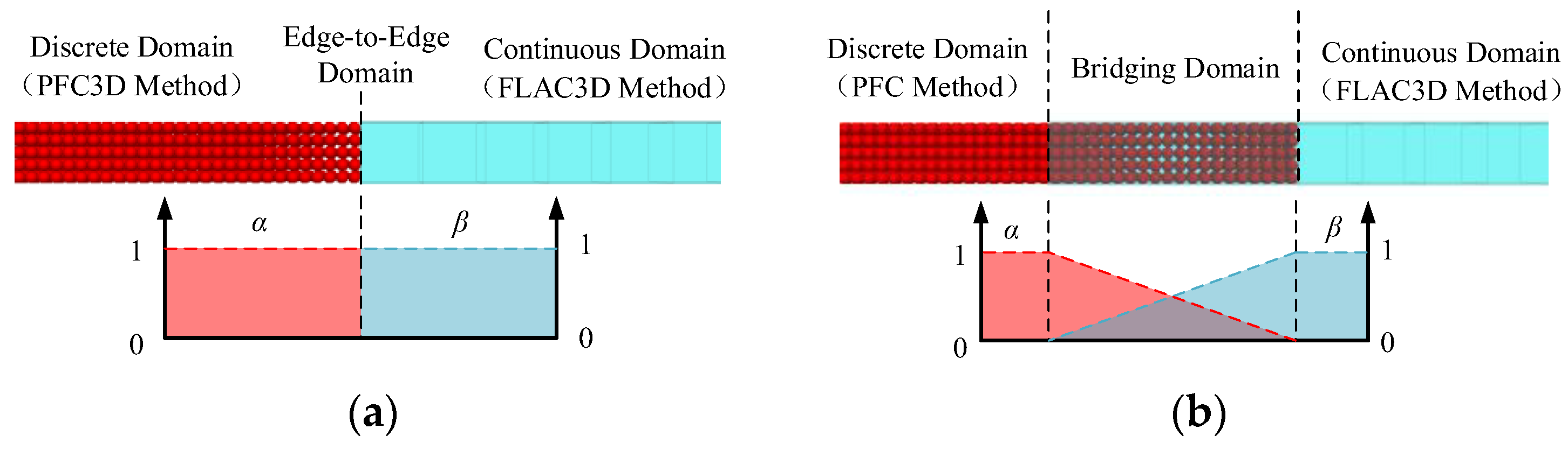
3.1. FLAC3D/PFC3D Coupled Theory

To ensure the continuity of the continuum-discrete medium regions, the continuous-discrete multi-scale coupling methods, based on the kinematics Hamiltonian operator H, are mainly divided into the edge-to-edge method and the bridging domain method [28,29]. The total system Hamiltonian energy H of the whole region studied is assumed to be divided into continuum system Hamiltonian energy HD (FLAC3D) and discrete media system Hamiltonian energy HC (PFC3D). To simplify the analysis and ensure the continuous energy transition, the linear combination coefficients α and β in the coupling region are defined.
H = α H D + β H C
The realization process of the edge-to-edge coupling method is to set the PFC model component wall on the surface of the FLAC model element, which may have a coupling effect, and it is used as the coupling variable exchange medium to accomplish the continuous and discontinuous coupling process.
The realization process of the bridging domain coupling method is to form a position superposition relationship in space between the FLAC model unit and particles in PFC, which is used as the exchange medium for coupling variables to realize continuous and discontinuous coupling processes. The bridging domain coupling method is shown in Figure 13b. In the discrete region, α and β are 1 and 0, respectively. In the continuous region, α and β are reversed. In the continuous-discrete coupling region, α and β increase or decrease linearly from 0 to 1. The bridging domain coupling method is mainly used for the dynamic analysis of models, so the continuous-discrete coupling method is adopted in this paper.

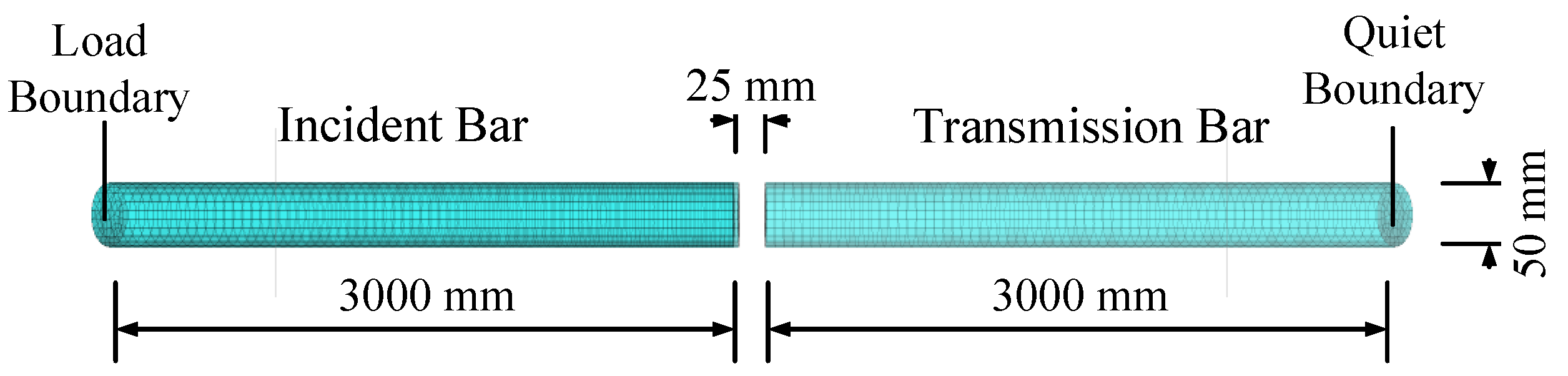
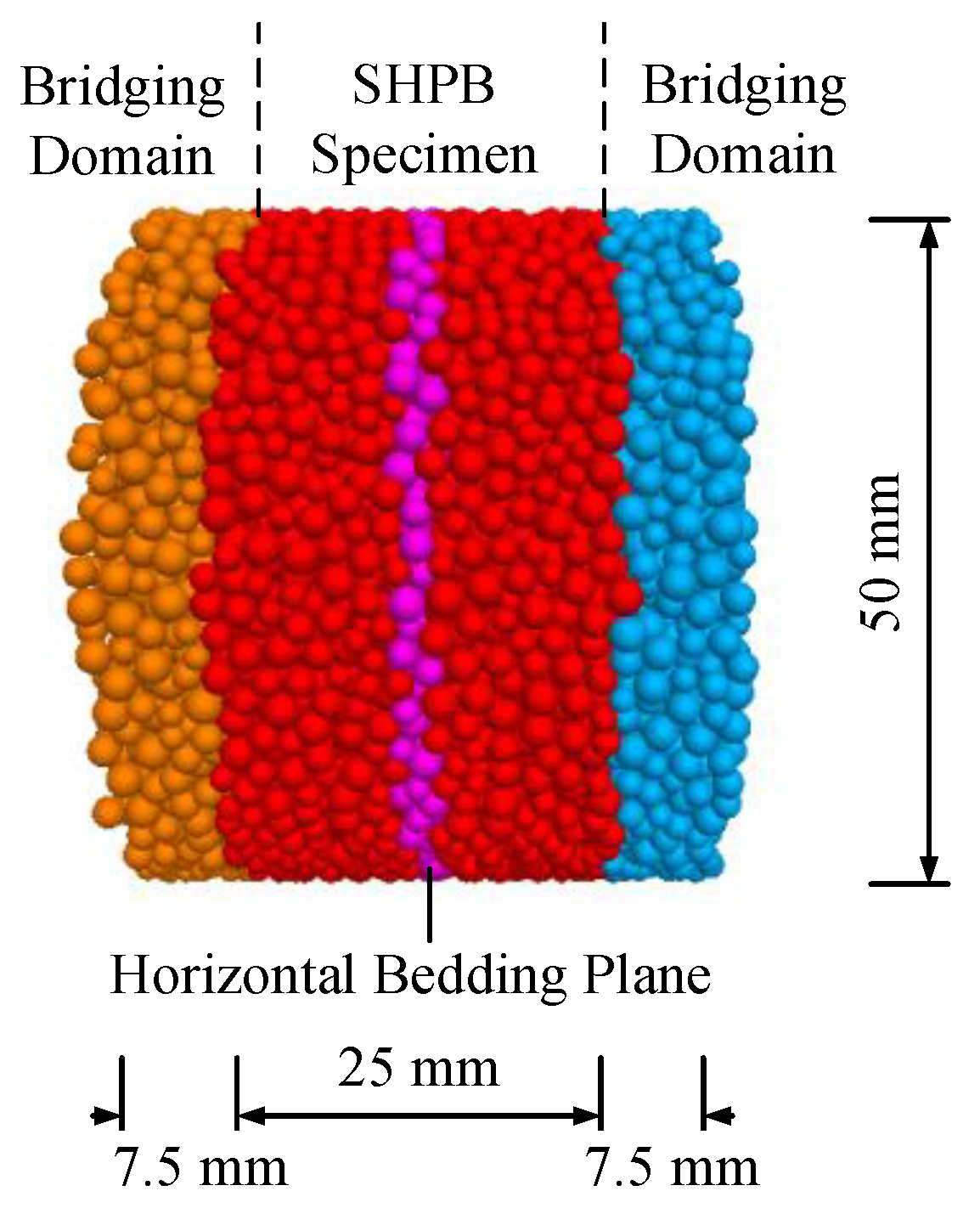
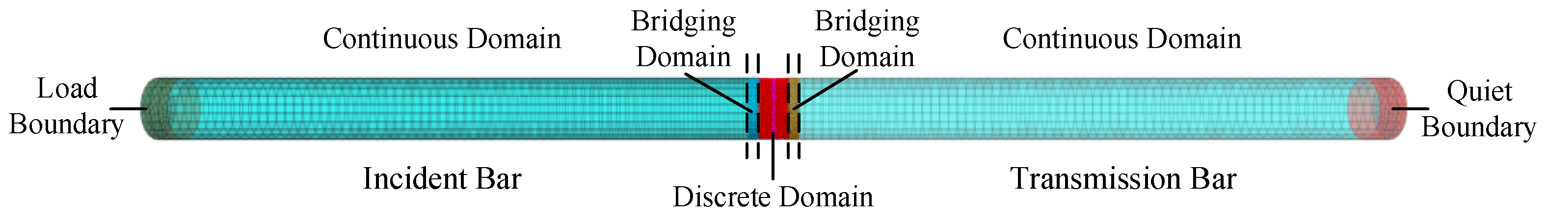
3.2. The Establishment of the SHPB Numerical Model

SolidWorks 2017 was used to establish the incident and transmission bar models. Then, the models were meshed in Abaqus 6.14, with a mesh size of 10 mm, and the meshed model was imported into FLAC3D 6.0. Finally, an incident bar and a transmission bar, with a diameter of 50 mm and a length of 3000 mm, were constructed. The distance between the incident bar and the transmission bar was 25 mm. The number of zones in the incident bar is 4032, and that in the transmission bar is 3864. The continuous area comprises 9656 nodes, as shown in Figure 14. The linear elastic model was adopted for the incidence and transmission bar. According to the material parameters of the SHPB test system, the density was 7.8 g/cm3, the elastic modulus was 206 GPa, and the Poisson ratio was 0.3. The left side of the incident bar is the loading boundary of the impact load, and the right side of the transmission bar is the quiet boundary, absorbing incident wave energy.
A rock discrete element sample with a diameter of 50 mm and a height of 40 mm was constructed through the PFC3D servo mechanism, as shown in Figure 15. The 7.5 mm range at both ends of the sample is the continuous-discrete coupling region. The 25 mm length in the middle of the sample is the SHPB specimen region. Since the limestone samples in the field are horizontal bedded samples, in order to ensure that the modeling is as close as possible to the samples in the field, the parallel bond model (PBM) is adopted to simulate the complete rock. Finally, the smooth joint model (SJM) is embedded in to generate the horizontally bedded rock samples. The porosity of the constructed sample is 0.3, the particle density ρ is 2.72 g/cm3, the maximum particle size Rmax is 10 mm, and the minimum particle size Rmin is 8 mm. The number of particles in the coupling region on both sides is 2029, and the number of particles in the middle SHPB specimen region is 9460. In the subsequent numerical tests, the micro-parameters used in the discrete-continuous coupling region and the SHPB specimen region are the same.
The bridging domain coupling method is used to couple the continuous model of the incident and the transmitted rod with the discrete model of the rock. Finally, the continuous-discrete SHPB model is constructed, as shown in Figure 16.

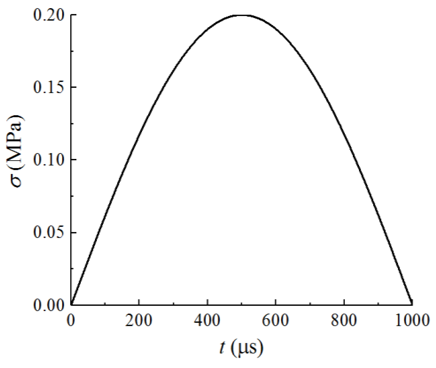
3.3. Impact Pressure Loading

For brittle rock materials, a half-sinusoidal loading wave can reduce waveform oscillation in the SHPB test and achieve approximately constant strain rate loading, which is an ideal loading waveform [30]. When conducting SHPB numerical tests, a half-sinusoidal loading wave, with a peak of 0.2 MPa and a duration of 1000 μs, was applied to the loading boundary of the incident rod, as shown in Figure 17.

4. Numerical Results and Discussion

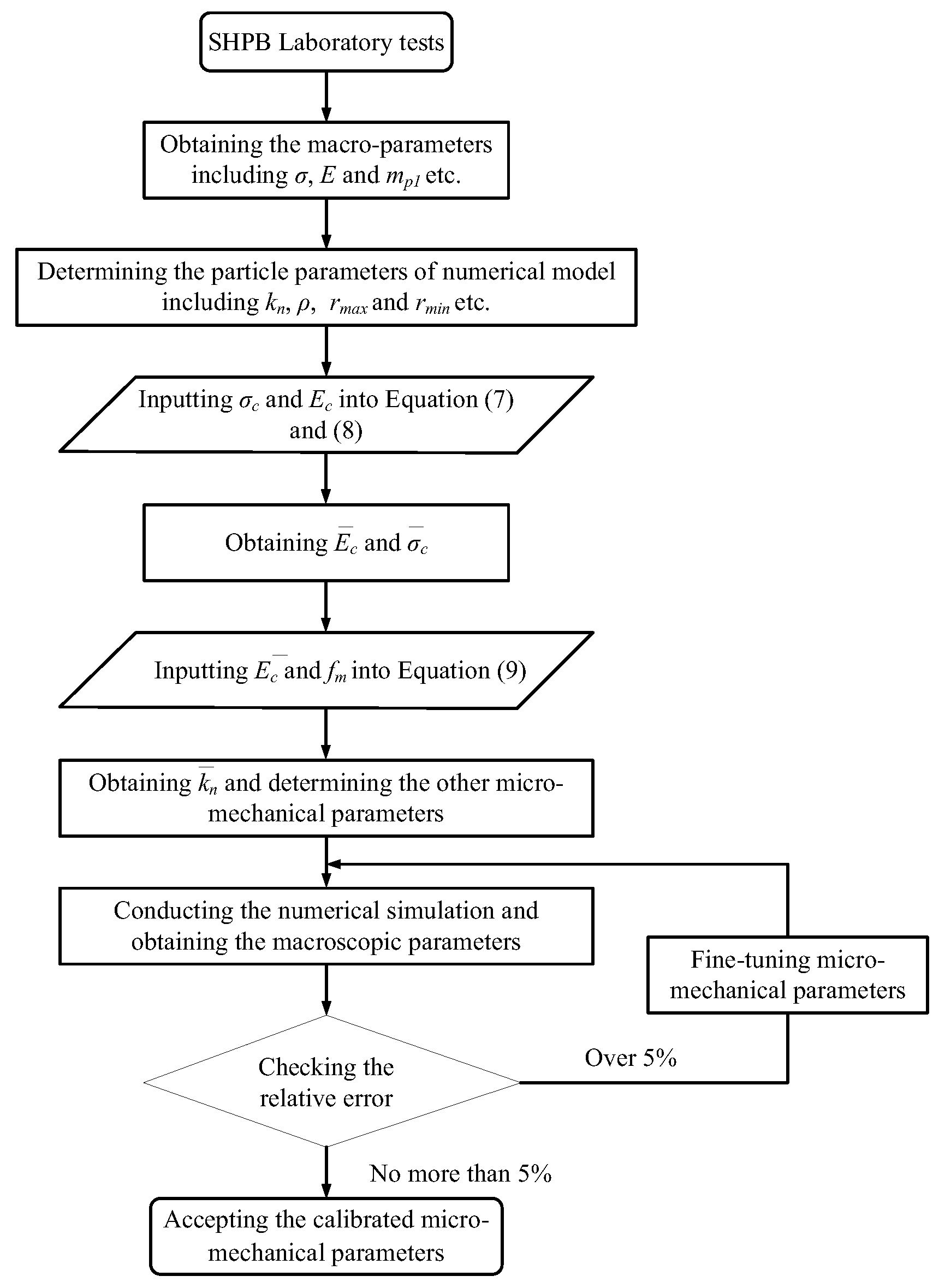
4.1. Selection of Particle Micro-Parameters

In the particle discrete element PFC3D software, the empirical quantitative relationship between the overall Young’s modulus of the model sample, the particle stiffness, and the particle radius is as follows [31]:
kn = 4rEc
where kn is the normal stiffness of the particles; r is the particle radius; Ec is the Young’s modulus of the sample.
In the SHPB model, the maximum particle size is 10 mm, and the minimum particle size is 8 mm. Take r in Equation (6) as the average radius; that is, r = 9 mm. Young’s dynamic modulus of the SHPB rock sample is 34.14 GPa, and Ec = 34.14 GPa. According to Equation (6), kn = 1.2 GPa can be calculated. Therefore, in subsequent numerical tests, the normal stiffness of particle kn is set to 1.2 GPa, and the ratio of normal stiffness to tangential stiffness kn/ks is 1.5.

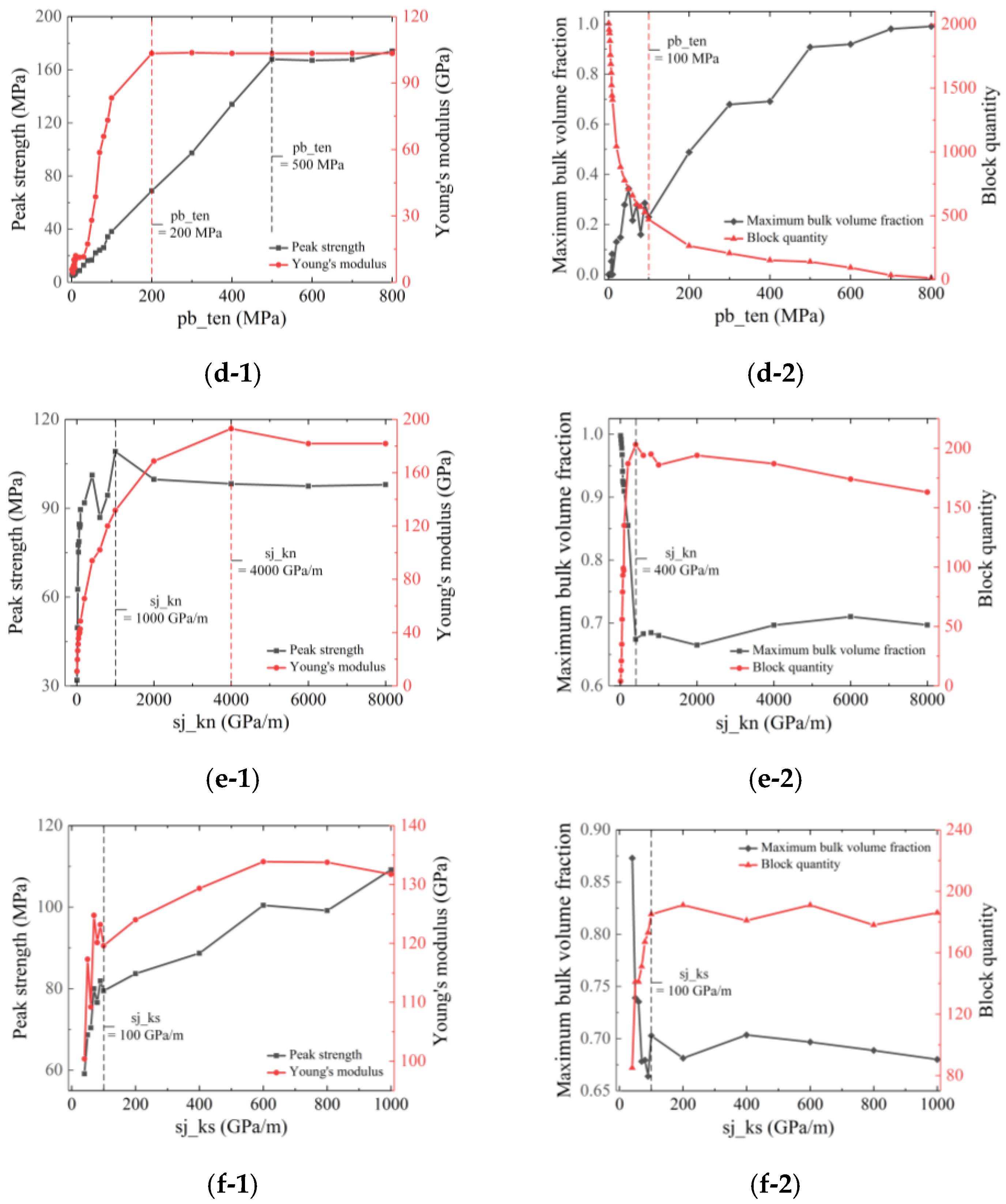
4.2. Analysis of SJM Micro-Parameters

In order to explore the influence of various microscopic parameters on macroscopic physical and mechanical parameters in the smooth joint model, six groups of numerical tests are set up in this section. The effects of six microscopic parameters, sj_fric μ, pb_deform emod E ¯ c , pb_coh σ ¯ c , pb_ten τ ¯ c , sj_kn k ¯ n , sj_ks k ¯ s , on the peak stress σp, the Young’s modulus of the sample Ec, the number of broken blocks, and the ratio of the maximum bulk volume to the total volume of the sample (maximum bulk volume fraction fm), respectively, were explored.
The values of the test variables and other micro-parameters in each group are shown in Table 2. The test results produced by the six groups of tests are shown in Figure 18.
According to the test results of group (a), as shown in Figure 18(a-1) and Figure 18(a-2), the changing trend of σp, Ec, and the number of broken blocks increases with the increase in μ. In contrast, the changing trend of fm decreases with the increase in μ. The larger the μ, the higher the degree of breakage of the sample under impact load.
According to the test results of group (b), as shown in Figure 18(b-1) and Figure 18(b-2), when E ¯ c ranges from 0.1 to 14 GPa, the variation trend of σp increases with the increase in E ¯ c . However, when E ¯ c >14 GPa, σp does not change much. When E ¯ c ranged from 0.1 to 150 GPa, Ec increased with the increase in E ¯ c , but when E ¯ c increased again, Ec did not change. The overall trend of fm decreases with the increase in E ¯ c , but when E ¯ c > 90 GPa, fm does not change much. The number of broken blocks increases with E ¯ c .
According to the test results of group (c), as shown in Figure 18(c-1) and Figure 18(c-2), when σ ¯ c ranges from 1 to 100 MPa, the changing trend of σp increases with σ ¯ c , but the change of σp is insignificant when σ ¯ c increases further. When σ ¯ c ranges from 1 MPa to 300 MPa, the changing trend of Ec increases with the increase in σ ¯ c , but the change of Ec is small when σ ¯ c increases further. When σ ¯ c ranges from 1 MPa to 200 MPa, the number of broken blocks increases with σ ¯ c , while for fm, the results are the opposite. However, when σ ¯ c > 200 MPa, the number of broken blocks and the fm do not change.
According to the test results of group (d), as shown in Figure 18(d-1) and Figure 18(d-2), when τ ¯ c is between 1 and 200 MPa, the changing trend of σp increases with the increase in σp, but when τ ¯ c increases further, the change in σp is small. When τ ¯ c is between 1 and 500 MPa, the changing trend of Ec increases with the increase in τ ¯ c , but the change of Ec is small when τ ¯ c increases further. The number of broken blocks increases with the increase in τ ¯ c , while the change trend of fm decreases with the increase in τ ¯ c .
According to the test results of group (e), shown in Figure 18(e-1) and Figure 18(e-2), when k ¯ n is 10–1000 GPa/m, the changing trend of σp increases, but when k ¯ n increases further, σp does not change much. When k ¯ n ranges from 10 to 4000 GPa/m, the changing trend of Ec increases with the increase in k ¯ n , but the Ec remains nearly unchanged when k ¯ n increases further. When k ¯ n is between 10 and 400 GPa/m, the number of broken blocks increases with k ¯ n , while for fm, the results are the opposite.
According to the test results for group (f), as shown in Figure 18(f-1) and Figure 18(f-2), the changing trend of σp and Ec increases with the increase in σp and Ec. When k ¯ s is in the range of 10~100 GPa/m, the number of broken blocks increases with the increase in k ¯ s , while for fm, the results are the opposite.

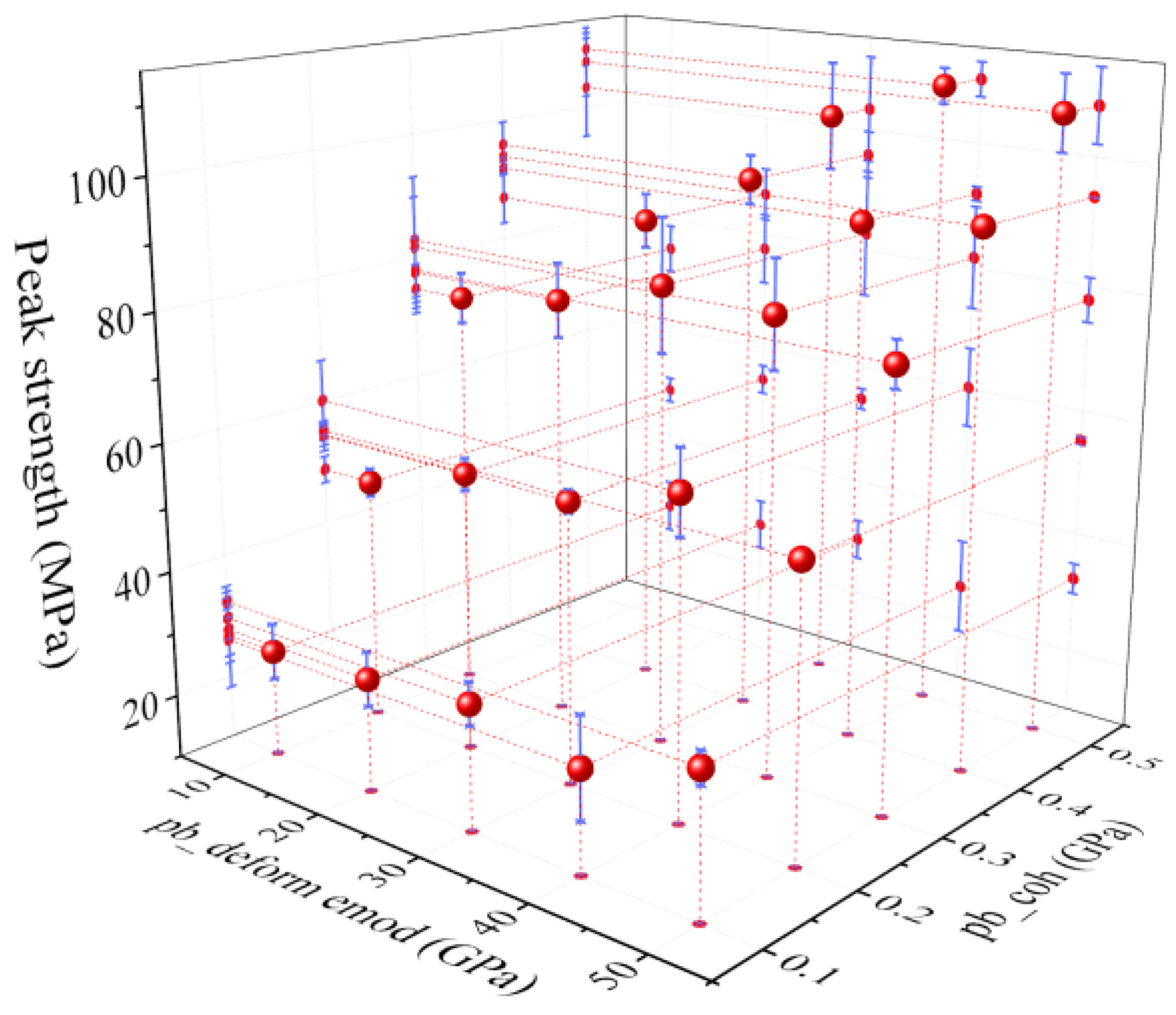
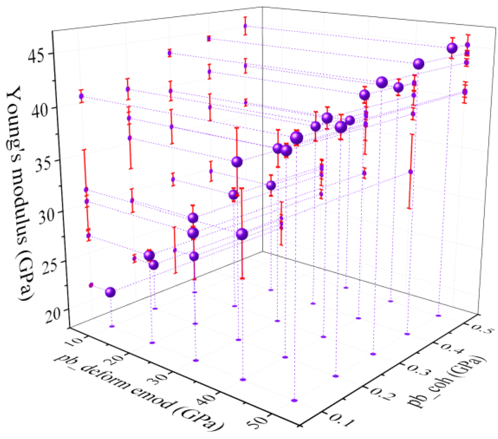
4.3. Micro-Parameters Calibration of Peak Stress and Young’s Modulus

According to the test results in Section 4.2, six micro-parameters, including μ and E ¯ c , influence the samples’ peak stress σp and Young’s modulus Ec. Since the influence of μ on σp, Ec, and fm are smaller than that of the other five micro-parameters on the macroscopic physical and mechanical parameters, μ is set at 0.15 in the subsequent study.
E ¯ c was set at 10, 20, 30, 40, and 50 GPa, and σ ¯ c was set at 0.1, 0.2, 0.3, 0.4, and 0.5 GPa. The results of the 21 orthogonal experiments are shown in Figure 19 and Figure 20. Since E ¯ c and σ ¯ c are mainly linearly related to sample σp and Ec, E ¯ c and σ ¯ c are used as double independent variables to carry out linear fitting for σp and Ec, respectively. The fitting formula is as follows:
σ p = 10.590 + 0.091 E ¯ c + 197.059 σ ¯ c R 2 = 0.962
E c = 15.606 + 0.458 E ¯ c + 15.190 σ ¯ c R 2 = 0.952
The residuals of σp and Ec obtained by linear fitting are shown in Figure 19 and Figure 20.

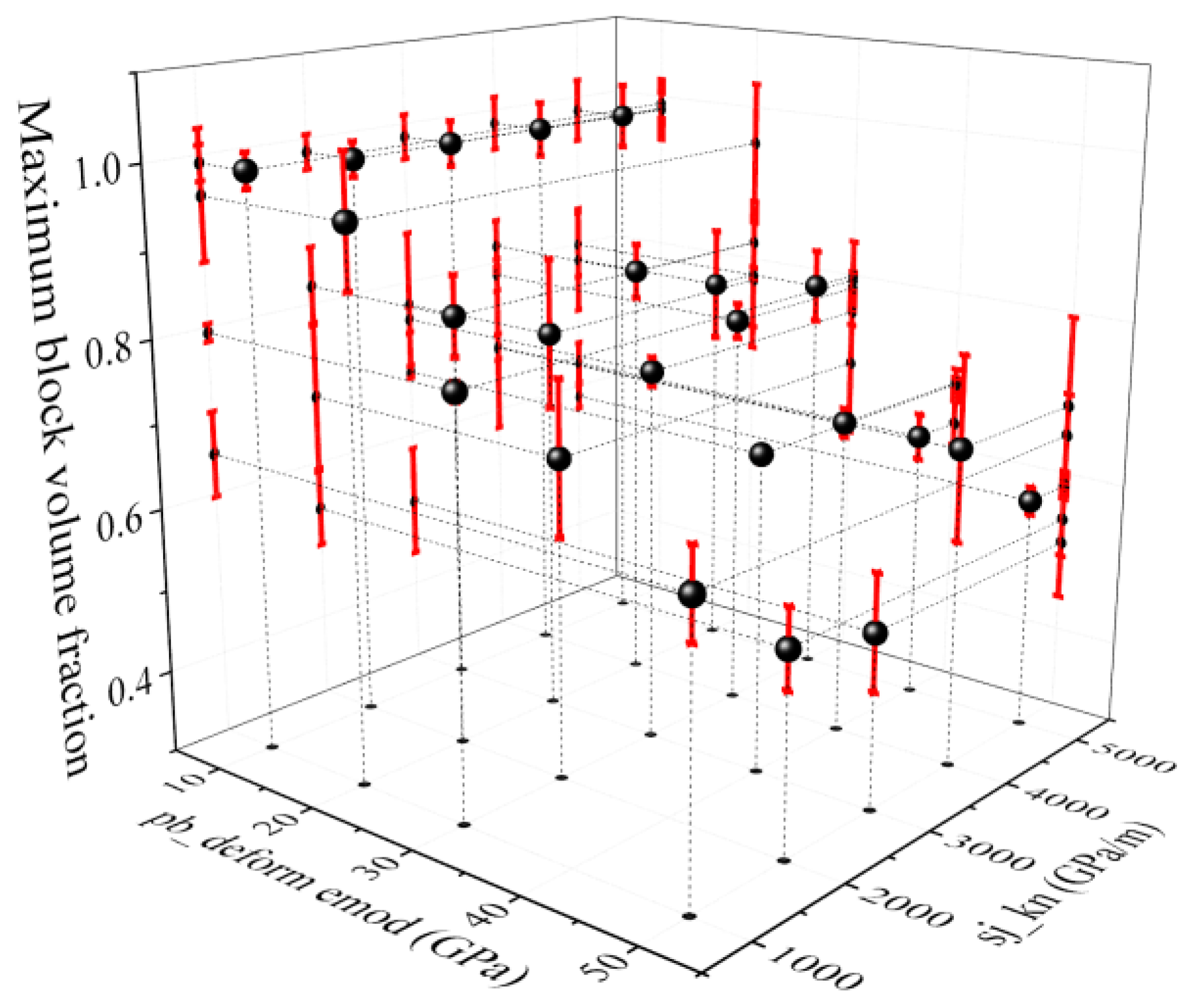
4.4. Micro-Parameters Calibration of Crushing Degree

According to the test results in Section 4.2, E ¯ c , σ ¯ c , and k ¯ n all have an impact on fm. However, when σ ¯ c is greater than 0.2 GPa, fm does not change. In order to reduce the variables, σ ¯ c is set as 0.3 GPa in this section. In summary, this section mainly carries out the quantitative analysis of E ¯ c and k ¯ n on fm.
Since σp and Ec no longer change when k ¯ n is greater than 1000 GPa/m, k ¯ n was set at1000, 2000, 3000, 4000, and 5000 GPa/m. E ¯ c was set at 10, 20, 30, 40, and 50 GPa. The results of the 23 orthogonal experiments are shown in Figure 21. Since E ¯ c and k ¯ n are mainly linearly related to fm, E ¯ c and k ¯ n are used as double independent variables to perform linear fitting on fm. The fitting formula is as follows:
f m = 1.070 0.009 E ¯ c 6.995   ×   10 6 k ¯ n R 2 = 0.861
The residual fm obtained by linear fitting is shown in Figure 21.

4.5. Final Calibration of Micro-Parameters

According to the test results in Section 4.3 and 4.4, the quantitative relationships between E ¯ c , σ ¯ c , and σp, Ec, and the quantitative relationships between E ¯ c , k ¯ n , and fm are obtained, respectively. Since E ¯ c influences the three macroscopic physical mechanics of the sample, E ¯ c should first be calibrated according to the compressive strength and Ec.
According to the SHPB test results in Section 2.3, the dynamic peak strength of the limestone sample is 84.29 MPa, the dynamic elastic modulus is 34.14 GPa, and the mass percentage of the maximum particle size group mpl is 0.78. When σp = 84.29, MPa and Ec= 34.14 GPa are substituted into Equations (7) and (8), and E ¯ c and σ ¯ c are 28.50 GPa and 0.36 GPa, respectively. If fm = mp1 = 0.78 and E ¯ c =28.50 GPa are substituted into Equation (9), k ¯ n is 4789.14 GPa/m. The names and values of the particle parameters, the PBM parameters, and the SJM parameters used are shown in Table 3.
The deviatoric stress–strain curves of the SHPB and PFC3D/FLAC3D numerical tests of limestone under an impact load of 0.2 MPa are shown in Figure 22. The dynamic compressive strength and the dynamic elastic modulus of the samples obtained from the numerical tests are 87.05 MPa and 33.11 GPa, respectively. The relative errors of the experimental results are 3.2% and 3%, respectively.
The fm obtained from the numerical test is 0.77, and the relative error from the laboratory test result mp1 is 1.3%. The final comparison of the failure modes is shown in Figure 23. The red disk represents the crack caused by shear failure. The blue disk represents the crack caused by tensile failure. It can be seen that the final failure modes of the two are similar.
The relative errors of compressive strength, elastic modulus, and the ratio of maximum bulk volume to total volume obtained from the numerical and laboratory tests are all less than 5%. Finally, the calibration of mesoscopic parameters is completed. The micro-parameter calibration program of the model based for the SHPB and PFC3D-FLAC3D method is shown in Figure 24.

5. Conclusions

Based on the SHPB test method and the FLAC3D/PFC3D numerical method, a continuous–discontinuous (FLAC3D/PFC3D) coupled SHPB numerical test model was established in this study. The quantitative relationship between the macroscopic physical and mechanical parameters and the microscopic parameters of SJM was determined and verified through many numerical tests. Finally, a calibration method for the micro-parameters of SJM under impact load is proposed, and the main conclusions are as follows:
(1)
Laboratory static physical and mechanical tests and SHPB tests were carried out on limestone samples to determine the macroscopic physical and mechanical parameters of the rock samples. At the same time, based on the SHPB laboratory test and the FLAC3D/PFC3D bridge domain coupling method, a continuous–discontinuous SHPB numerical test model is established.
(2)
Through univariate analysis, the influence between six micro-parameters of the numerical model and the macroscopic physical and mechanical parameters are explored, and the microscopic parameters of SJM to be calibrated are simplified into three types, namely pb_deform emod E ¯ c , pb_coh σ ¯ c , and sj_kn k ¯ n . Then, the quantitative relationships between the three micro-parameters and the three macro-physical and mechanical parameters were established by two-factor regression analysis.
(3)
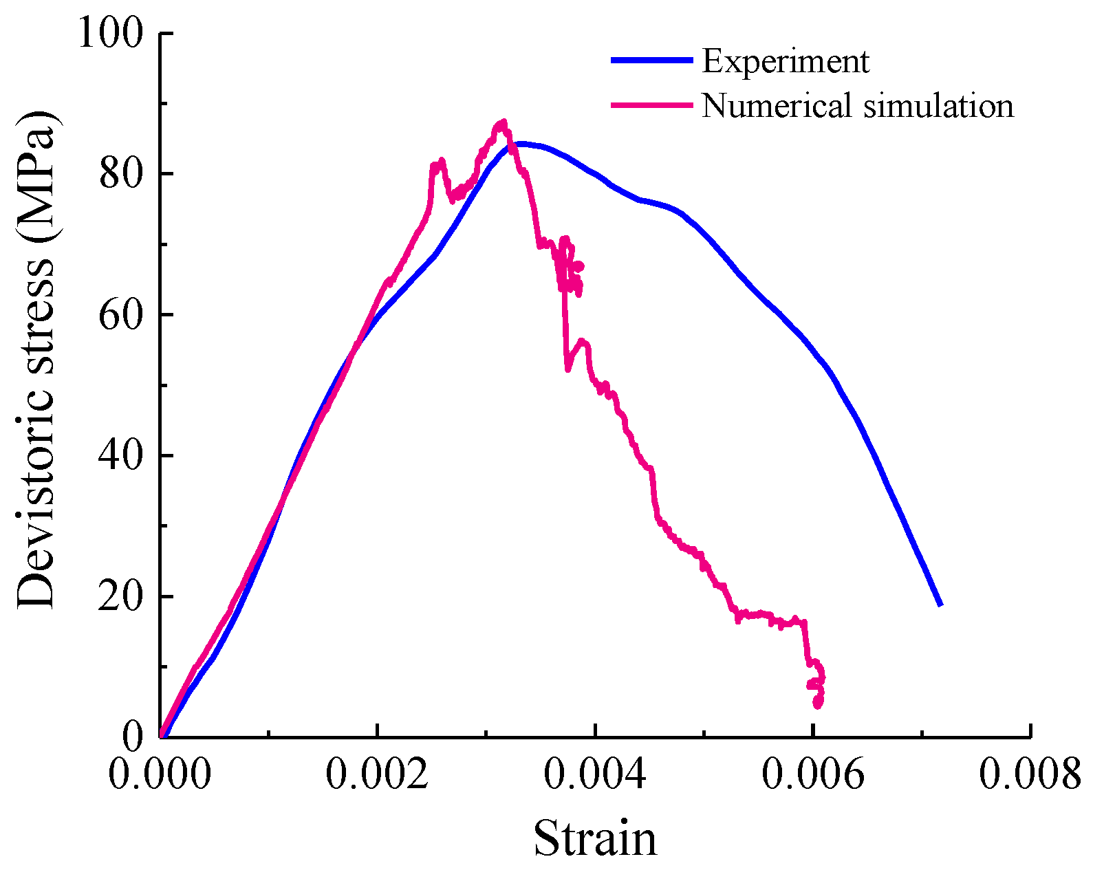
The calibration process for the microscopic parameters of SJM under impact load was established, and the quantitative relationship between microscopic and macroscopic parameters was verified according to the SHPB test. The relative error of the macroscopic parameters between the numerical and laboratory tests is less than 5%, which shows that the proposed calibration method is more accurate and reliable than previous methods. At the same time, compared with the traditional calibration method of trial and error, the calibration efficiency of the micro-parameters is improved.
(4)
This paper provides a more reliable continuous–discontinuous numerical model for the SHPB test and also provides the calibration process for the model’s microscopic parameters, which supplies a certain reference value for the study of the rock model under impact load. Due to the limited number of experiments conducted in this study, it is necessary to increase this number in the future to fully validate the calibration process.

Author Contributions

Methodology, Z.Z.; software, Y.K.; writing—original draft preparation, W.G. All authors have read and agreed to the published version of the manuscript.

Funding

This research was funded by National Natural Science Foundation of China, (Study on rock breaking process and mechanism of cutting blasting in deep high-stress rock roadway) grant number 51874189.

Institutional Review Board Statement

Not applicable.

Informed Consent Statement

Not applicable.

Data Availability Statement

The data presented in this study are available on request from the corresponding author. The data are not publicly available due to the privacy of the data.

Acknowledgments

The support from Chao Wu and Rangang Yu in the form of their guidance and assistance in the writing of this paper is gratefully acknowledged.

Conflicts of Interest

The authors declare no conflict of interest.

References

  1. Castro-Filgueira, U.; Alejano, L.R.; Arzúa, J.; Ivars, D.M. Sensitivity Analysis of the Micro-Parameters Used in a PFC Analysis Towards the Mechanical Properties of Rocks. Procedia Eng. 2017, 191, 488–495. [Google Scholar] [CrossRef]
  2. Xu, Z.H.; Wang, W.Y.; Lin, P.; Xiong, Y.; Liu, Z.Y.; He, S.J. A parameter calibration method for PFC simulation. Development and a case study of limestone. Geomech. Eng. 2020, 22, 97–108. [Google Scholar]
  3. Li, Z.; Rao, Q. Quantitative determination of PFC3D microscopic parameters. J. Cent. South Univ. 2021, 28, 911–925. [Google Scholar] [CrossRef]
  4. Ajamzadeh, M.R.; Sarfarazi, V.; Haeri, H.; Dehghani, H. The effect of micro parameters of PFC software on the model calibration. Smart Struct. Syst. 2018, 22, 643–662. [Google Scholar] [CrossRef]
  5. Xu, Z.; Wang, Z.; Wang, W.; Lin, P.; Wu, J. An integrated parameter calibration method and sensitivity analysis of microparameters on mechanical behavior of transversely isotropic rocks. Comput. Geotech. 2022, 142, 104573. [Google Scholar] [CrossRef]
  6. Su, H.; Li, H.; Hu, B.; Yang, J. A research on the macroscopic and mesoscopic parameters of concrete based on an experimental design method. Materials 2021, 14, 1627. [Google Scholar] [CrossRef] [PubMed]
  7. Shi, C.; Yang, W.; Yang, J.; Chen, X. Calibration of micro-scaled mechanical parameters of granite based on a bonded-particle model with 2D particle flow code. Granul. Matter 2019, 21, 38. [Google Scholar] [CrossRef]
  8. Yoon, J. Application of experimental design and optimization to PFC model calibration in uniaxial compression simulation. Int. J. Rock Mech. Min. Sci. 2007, 44, 871–889. [Google Scholar] [CrossRef]
  9. Wu, H.; Dai, B.; Zhao, G.; Chen, Y.; Tian, Y. A Novel Method of Calibrating Micro-Scale Parameters of PFC Model and Experimental Validation. Appl. Sci. 2020, 10, 3221. [Google Scholar] [CrossRef]
  10. Zou, Q.; Lin, B. Modeling the relationship between macro-and meso-parameters of coal using a combined optimization method. Environ. Earth Sci. 2017, 76, 479. [Google Scholar] [CrossRef]
  11. Tatone, B.S.; Grasselli, G. A calibration procedure for two-dimensional laboratory-scale hybrid finite–discrete element simulations. Int. J. Rock Mech. Min. Sci. 2015, 75, 56–72. [Google Scholar] [CrossRef]
  12. Cheng, K.; Wang, Y.; Yang, Q.; Mo, Y.; Guo, Y. Determination of microscopic parameters of quartz sand through tri-axial test using the discrete element method. Comput. Geotech. 2017, 92, 22–40. [Google Scholar] [CrossRef]
  13. Zhao, Y.; Zhao, G.-F.; Jiang, Y.; Elsworth, D.; Huang, Y. Effects of bedding on the dynamic indirect tensile strength of coal: Laboratory experiments and numerical simulation. Int. J. Coal Geol. 2014, 132, 81–93. [Google Scholar] [CrossRef]
  14. Ai, D.; Zhao, Y.; Wang, Q.; Li, C. Crack propagation and dynamic properties of coal under SHPB impact loading: Experimental investigation and numerical simulation. Theor. Appl. Fract. Mech. 2019, 105, 102393. [Google Scholar] [CrossRef]
  15. Kong, X.; Wang, E.; Li, S.; Lin, H.; Zhang, Z.; Ju, Y. Dynamic mechanical characteristics and fracture mechanism of gas-bearing coal based on SHPB experiments. Theor. Appl. Fract. Mech. 2019, 105, 102395. [Google Scholar] [CrossRef]
  16. Li, J.C.; Rong, L.F.; Li, H.B.; Hong, S.N. An SHPB Test Study on Stress Wave Energy Attenuation in Jointed Rock Masses. Rock Mech. Rock Eng. 2019, 52, 403–420. [Google Scholar] [CrossRef]
  17. Li, C.; Wang, Q.; Lyu, P. Study on electromagnetic radiation and mechanical characteristics of coal during an SHPB test. J. Geophys. Eng. 2016, 13, 391–398. [Google Scholar] [CrossRef]
  18. Gong, F.; Jia, H.; Zhang, Z.; Hu, J.; Luo, S. Energy Dissipation and Particle Size Distribution of Granite under Different Incident Energies in SHPB Compression Tests. Shock Vib. 2020, 2020, 8899355. [Google Scholar] [CrossRef]
  19. Guo Ren, H.; Zhang, L.; Long, Z.; Wu, X.; Wang, H. Research of an SHPB Device in Two-by-Two Form for Impact Experiments of Concrete-Like Heterogeneous Materials. Acta Mech. Solida Sin. 2021, 34, 561–581. [Google Scholar] [CrossRef]
  20. Li, D.; Han, Z.; Sun, X.; Zhou, T.; Li, X. Dynamic Mechanical Properties and Fracturing Behavior of Marble Specimens Containing Single and Double Flaws in SHPB Tests. Rock Mech. Rock Eng. 2019, 52, 1623–1643. [Google Scholar] [CrossRef]
  21. Ping, Q.; Fang, Z.; Ma, D.; Zhang, H. Coupled Static-Dynamic Tensile Mechanical Properties and Energy Dissipation Characteristic of Limestone Specimen in SHPB Tests. Adv. Civ. Eng. 2020, 2020, 7172928. [Google Scholar] [CrossRef]
  22. Qiu, J.; Li, D.; Li, X.; Zhou, Z. Dynamic Fracturing Behavior of Layered Rock with Different Inclination Angles in SHPB Tests. Shock Vib. 2017, 2017, 7687802. [Google Scholar] [CrossRef]
  23. Wang, T.; Song, Z.; Yang, J.; Zhang, Q.; Cheng, Y. A Study of the Dynamic Characteristics of Red Sandstone Residual Soils Based on SHPB Tests. KSCE J. Civ. Eng. 2021, 25, 1705–1717. [Google Scholar] [CrossRef]
  24. Yang, Z.; Fan, C.; Lan, T.; Li, S.; Wang, G.; Luo, M.; Zhang, H. Dynamic Mechanical and Microstructural Properties of Outburst-Prone Coal Based on Compressive SHPB Tests. Energies 2019, 12, 4236. [Google Scholar] [CrossRef]
  25. Ping, Q.; Ma, Q.Y.; Yuan, P. Energy dissipation analysis of stone specimens in shpb tensile test. Caikuang Yu Anquan Gongcheng Xuebao/J. Min. Saf. Eng. 2013, 30, 401–407. [Google Scholar]
  26. Zou, H.R.; Yin, W.L.; Cai, C.C.; Yang, Z.; Li, Y.B.; He, X.D. Numerical Investigation on the Necessity of a Constant Strain Rate Condition According to Material’s Dynamic Response Behavior in the SHPB Test. Exp. Mech. 2019, 59, 427–437. [Google Scholar] [CrossRef]
  27. Wang, S. Study on Blasting Fragmentation Distribution Law and Blasting Parameters Optimization in Open-Pit Coal Mine. Ph.D. Thesis, China University of Mining and Technology, Xuzhou, China, 2020. (In Chinese) [Google Scholar] [CrossRef]
  28. Li, M.; Yu, H.; Wang, J.; Yuan, Y.; Chen, J. Bridging Coupled Discrete-continuum Multi-scale Approach for Dynamic Analysis. Eng. Mech. 2013, 32, 92–98. (In Chinese) [Google Scholar] [CrossRef]
  29. Breugnot, A.; Lambert, S.; Villard, P.; Gotteland, P. A Discrete/continuous Coupled Approach for Modeling Impacts on Cellular Geostructures. Rock Mech. Rock Eng. 2015, 49, 1831–1848. [Google Scholar] [CrossRef]
  30. Panowicz, R.; Janiszewski, J.; Kochanowski, K. Numerical and Experimental Studies of a Conical Striker Application for the Achievement of a True and Nominal Constant Strain Rate in SHPB Tests. Exp. Mech. 2018, 58, 1325–1330. [Google Scholar] [CrossRef]
  31. Itasca Consulting Group Inc. PFC3D-Particle Flow Code 3 Dimension; Ver. 4.0; User’s Manual; Itasca Consulting Group Inc.: Minneapolis, MN, USA, 2010. [Google Scholar]
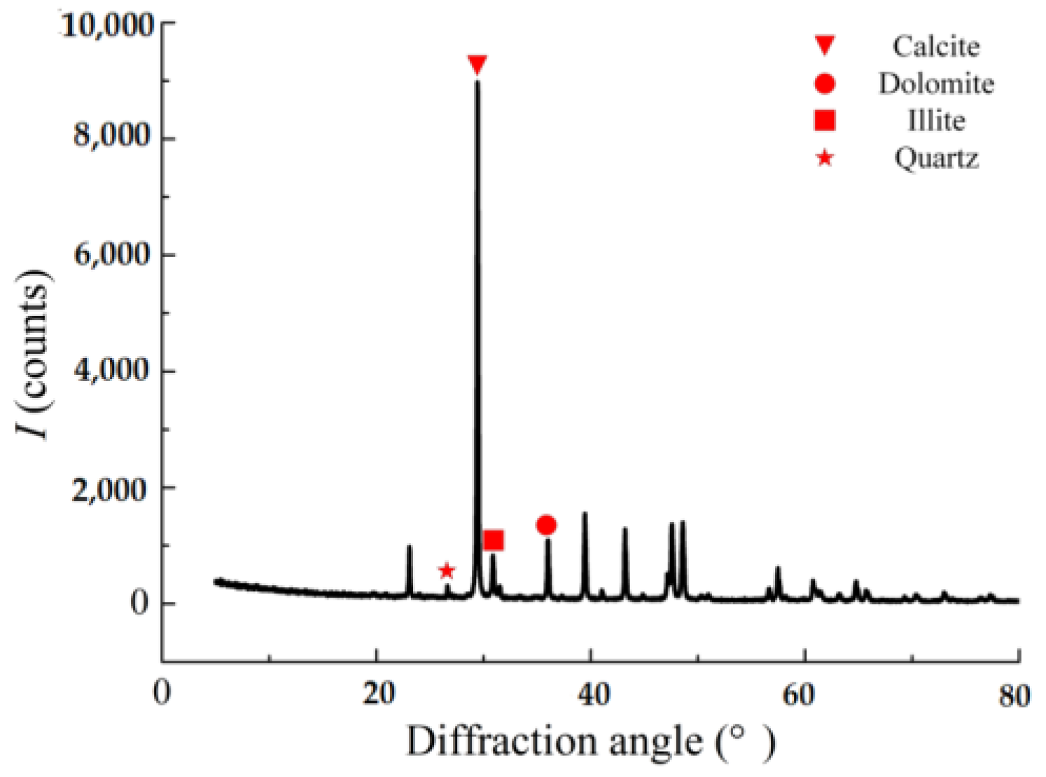
Figure 1. Limestone UCS specimen.
Applsci 14 03020 g001
Figure 2. Limestone SHPB specimen.
Applsci 14 03020 g002
Figure 3. XRD pattern of limestone.
Applsci 14 03020 g003
Figure 4. TAW-1000 Pressure servo test system.
Applsci 14 03020 g004
Figure 5. Deviatoric stress–axial and radial strain curves.
Applsci 14 03020 g005
Figure 6. SHPB test system.
Applsci 14 03020 g006
Figure 7. A sample of limestone in a clamped state.
Applsci 14 03020 g007
Figure 8. Typical three-wave original waveform.
Applsci 14 03020 g008
Figure 9. Deviatoric stress–strain curve when the impact pressure is 0.2 MPa.
Applsci 14 03020 g009
Figure 10. Failure modes of rock samples under uniaxial compression at an impact pressure of 0.2 MPa.
Applsci 14 03020 g010
Figure 11. Grading screen for sample fragments.
Applsci 14 03020 g011
Figure 12. Fragment characteristics of rock samples.
Applsci 14 03020 g012
Figure 13. Continuous-discrete (FLAC3D/PFC3D) coupling model: (a) edge-to-edge method; (b) bridging domain method.
Applsci 14 03020 g013
Figure 14. FLAC3D model of the incident bar and transmission bar.
Applsci 14 03020 g014
Figure 15. PFC3D model of SHPB rock sample with horizontal bedding.
Applsci 14 03020 g015
Figure 16. Continuous-discrete (FLAC3D/PFC3D) SHPB model.
Applsci 14 03020 g016
Figure 17. Half-sine loading wave.
Applsci 14 03020 g017
Figure 18. Experimental results for groups (af).
Applsci 14 03020 g018aApplsci 14 03020 g018b
Figure 19. The test results of pb_deform emod E ¯ c and pb_coh   σ   ¯ c for peak stress σp of the sample and the fitting residual.
Applsci 14 03020 g019
Figure 20. The test results of pb_deform emod E ¯ c and pb_coh σ ¯ c for Young’s modulus Ec of the sample and the fitting residual.
Applsci 14 03020 g020
Figure 21. Test results and fitted residuals of E ¯ c and k ¯ n on fm.
Applsci 14 03020 g021
Figure 22. Comparison of deviatoric stress–strain curves between laboratory and numerical tests.
Applsci 14 03020 g022
Figure 23. Comparison of failure modes.
Applsci 14 03020 g023
Figure 24. Micro-parameter calibration flow of SJM under impact load.
Applsci 14 03020 g024
Table 1. Measurement results of limestone quantitative composition.
Main
Ingredients
QuartzPotassium FeldsparDolomiteCalciteIlliteOther Clay Minerals
%0.407.889.51.21.1
Table 2. Micro-parameters in (a)~(f) group.
Groupμ E ¯ c (GPa) σ ¯ c (GPa) τ ¯ c (GPa) k ¯ n (GPa/m) k ¯ s (GPa/m)
(a)0.01~0.99250.520.3210001000
(b)0.150.1~2000.520.3210001000
(c)0.15251~0.80.3210001000
(d)0.15250.521~0.810001000
(e)0.15250.520.3210~80001000
(f)0.15250.520.32100010~1000
Table 3. Names and values of each micro-parameter.
BallValuePBMValueSJMValue
kn (GPa)1.2 E ¯ c (GPa)28.50 k ¯ n (GPa/m)4789.14
kn/ks1.5 σ ¯ c (GPa)0.36 k ¯ s (GPa/m)4789.14
Rmax (mm)10 τ ¯ c (GPa)0.36sj_coh σc (MPa)3
Rmin (mm)8Kratio k ¯ n / k ¯ s 1.5sj_ten τc (MPa)2
ρ (g/cm3)2.72 μ0.15
Disclaimer/Publisher’s Note: The statements, opinions and data contained in all publications are solely those of the individual author(s) and contributor(s) and not of MDPI and/or the editor(s). MDPI and/or the editor(s) disclaim responsibility for any injury to people or property resulting from any ideas, methods, instructions or products referred to in the content.

