Article

Last Glacial Maximum Climate and Glacial Scale Affected by the Monsoon Inferred from Reconstructing the Tianchi Area, Changbai Mountains, Eastern China

School of Geographical Sciences, Liaoning Normal University, Dalian 116021, China
*
Author to whom correspondence should be addressed.
Appl. Sci. 2024, 14(7), 3019; https://doi.org/10.3390/app14073019
Submission received: 6 February 2024 / Revised: 29 March 2024 / Accepted: 2 April 2024 / Published: 3 April 2024

Abstract

:
There are few studies on the climate and glacial scale in the mountains east of the Qinghai–Tibet Plateau. So, we used glacial features to determine the range of the area’s paleoglaciers and the equilibrium line altitude (ELA) of theGlA modern and paleoglaciers in the Tianchi area of the Changbai Mountains. Then, the GlaRe toolbox 2015 () was used to reconstruct the surface of the paleoglaciers. The probable air temperature during the glacial advances of the LGM was calculated by applying the P-T and LR models. The results showed the following: (1) the change in ELA is 950 m in the Tianchi area of the Changbai Mountains; (2) glacial coverage in the Tianchi area of the Changbai Mountains during the LGM period was ~27.05 km2 and the glacial volume was ~9.94 km3; and (3) the mean temperature in the Tianchi area of the Changbai Mountains during the LGM was 6.6–9.0 °C lower than today’s, and was the principal factor controlling the growth of glaciers. There is a difference in the climate change in monsoon-influenced mountains during the LGM, and this difference may be related to the precipitation in the mountains.

1. Introduction

Climate change can lead to changes in the shape, area and volume of mountain glaciers [1,2,3,4,5]. Therefore, glacial landforms with chronological evidence (e.g., terminal and lateral moraine ridges) can be used to reconstruct paleoglacial surfaces as well as paleoclimatic features for specific periods [6,7,8,9]. The Last Glacial Maximum (LGM) is the closest extreme cold period to modern times. Globally, there was massive sea retreat accompanied by a dry and cold climate. Glaciation occurred on the Tibetan Plateau (TP) and its surrounding mountains during the Last Glacial Maximum (LGM), as well as in the coastal mountains of East Asia, but the magnitude of this glaciation varied [10,11,12,13]. Although environmental changes followed roughly similar patterns globally, different regions experienced differing magnitudes of glaciation and climate change [14,15]. It is therefore important to study the LGM’s climatic and environmental characteristics in order to clarify how temperature and precipitation drove glacial advances and leaded to climate change. Analyzing the extent to which there was environmental heterogeneity between different regions is key to understanding climate change today [16]. However, current paleoclimate reconstructions in the LGM are mainly focused on the Tibetan Plateau and its surrounding mountain ranges [17,18,19,20,21,22,23], and there are few relevant studies for the mountainous regions of eastern China [24], which hinders the comparison of LGM climate change between the Tibetan Plateau and other mountainous regions.
The development of glaciers in eastern China is closely related to the influence of the East Asian monsoon (EAM) [13]. Since the influence of the monsoon on the climatic and geomorphological environment of the Quaternary Period is particularly relevant to the history of the global ice age change [11], the quantification of the paleoglaciers and paleoclimate in the eastern Tibetan Plateau during the LGM can provide a better understanding of climate change in eastern China, and is of great significance for understanding the paleoenvironment under the influence of the East Asian monsoon. The Tianchi area of the Changbai Mountains, representative of a once-glaciated area within this EAM-controlled environment of East Asia, is sensitive to global environmental change. The Tianchi area of the Changbai Mountains contains a rich archive of glacial relics; however, there are no quantitative reconstruction studies of the paleoclimate in this study area. In order to bridge this gap, we firstly reconstructed the paleoglacial surface of the LGM in the Tianchi area. Then, we calculated the the equilibrium line altitude (ELA) values for the LGM as well as for the modern era. And, finally, we inferred the paleoclimate of the Tianchi area during the LGM by using the ELA-related climate models (P-T and LR models) in combination with data from high-elevation meteorological stations. In addition, possible climatic driving factors during the LGM in the Tianchi area are discussed. The paleoclimate reconstruction results of this study area are statistically analyzed with those of the mountainous areas affected by the East Asian monsoon and the Indian monsoon, in order to identify the common features of the paleoclimate variations under the influence of the monsoon.

2. Study Area

The Changbai Mountains constitute the northernmost mountainous area in eastern China where Quaternary glaciers developed. Their geographic location is unique in that they link the Chinese Loess Plateau (CLP) to the Sea of Japan and its islands laterally; longitudinally, they connect Russia’s Far East, China’s vast sea area and Taiwan. Located on the eastern edge of the Eurasian Plate near the coast of the Western Pacific Ocean, Tianchi is the famous volcanic crater lake of the Changbai Mountains (Figure 1). The study area is located on the east coast of the Eurasian continent in the mid-latitudes. EAM-controlled westerly winds dominate its temperate climate throughout the year. The climate is windy in spring, warm for a short period in summer, foggy and cool in autumn and extremely cold in winter. According to the records of the Tianchi meteorological station (2623 m) over many years, the average temperature in spring is −8 °C, in summer is 7 °C, in autumn is −10 °C and in winter is −23 °C. The growing season is short. The highest temperature (T) in the Tianchi area of the Changbai Mountains occurs in July and the lowest in January. Most precipitation (P) in the Tianchi area falls in July, with the lowest amounts recorded in January. The EAM circulation controls P in this study area, resulting in an uneven seasonal distribution of P, with the summer months accounting for ~60–70% of total annual P [25,26].
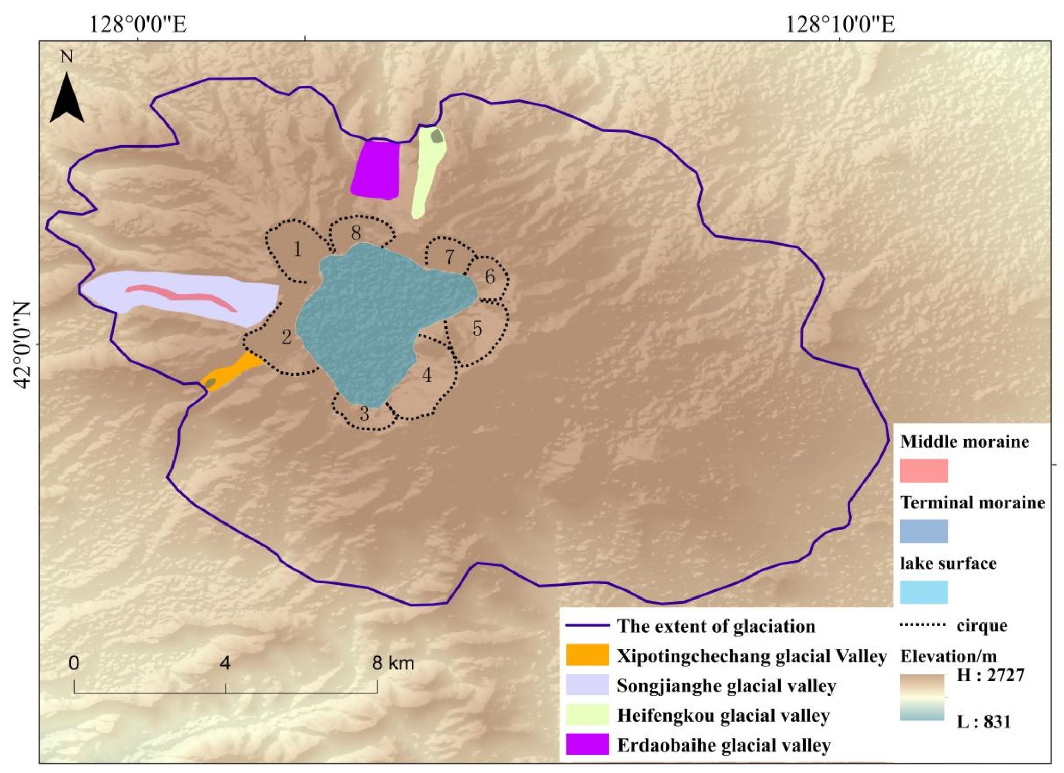
The authors’ field surveys and previous studies [10,11,27] have identified the main types of glacial remnants preserved in the area. These include cirques, glacial valleys, terminal moraine ridges and medial moraine ridges. Eight cirques can be found in the study area, principally in the caldera; here, the mean altitude of the base of the cirques is 2239 m asl (Table 1). Typical glaciated valleys include the Heifengkou and Erdaobaihe valleys on the north-facing slopes of the Changbai Mountains and the Xipotingchechang and Songjianghe valleys on the west-facing slopes. The Heifengkou and Xipotingchechang valleys contain well-preserved terminal moraine ridges. There are also well-preserved medial moraine ridges in the Songjianghe Valley (Figure 2). The lower limit of the glacial remnants of the LGM in the study area is 1850 m asl [13,26]. Li [28] considered that the last Quaternary glaciation in the Tianchi area occurred during the LGM. Qiu [12] also believed that the last glaciation in this area was during the LGM. Zhang [27] conducted a chronological study of two sets of moraines preserved in the Tianchi area of the Changbai Mountains using optically stimulated luminescence (OSL) dating techniques and determined that there were glacial advances in both the LGM (~20 ka) and the Last Glacial Period (LGP; 11 ka).

3. Materials and Methods

The base topography we inputted was obtained from a calibrated 30 m resolution ASTER GDEM V2 dataset (http://www.gscloud.cn/) (accessed 19 December 2023). The meteorological data used in this article come from the China Meteorological Data Sharing Service System (http://www.nmic.cn) (accessed on 8 October 2023).

3.1. Quantitative Recovery of Glacier Size

The reconstruction of the glacier size in the study area during a period of glacial advance primarily focuses on glacier coverage, depth and volume. The most commonly used simulation method for such reconstructions is the glacial longitudinal line model [29,30,31,32,33,34], based on geomorphological information from the glacial action area and the glacial dynamics equation; thus:
τ = ρ g H sin α
where τ is shear stress (Pa), ρ is the density of glacial ice (~900 kg−3), g is the gravitational acceleration (9.81 ms−2), H is the thickness of the glacier (m) and α is the slope (gradient) of the glacier surface. In addition, the movement of glaciers in the valley is also affected by the lateral drag of the valley. Therefore, it is necessary to incorporate the F-factor (shape friction factor) into the equation, and the equation for the base shear stress after adjustment is:
τ a = ρ g F H sin α
F = A H p
where A is the area of the glacier cross-section (m2) and p is perimeter of the cross-section (m) [35].
Equation (2) is derived into a quadratic equation, Equation (4) [29,36], which can be solved iteratively along the central glacier flow line:
h i + 1 2 h i + 1 b i + b i + 1 + h i b i + 1 H i 2 Δ x τ a v F g = 0
where h is the ice surface elevation (m), b is the glacier bed elevation (m), Δx is the step length (m), τ a v is the average basal shear stress over an interval (Pa) and i is the iteration step number. Glacier-scale reconstruction can be carried out using the GlaRe tool [37,38]. And this tool has been applied to the reconstruction of paleoglacial surfaces in other areas [39].

3.2. Determining the ELA

3.2.1. Calculating the ELAm of Modern Glaciers

The study area’s modern ELAm values were used to reconstruct the paleoclimate. Taking into account the relationship between P and T, two methods can be used to quantitatively calculate the ELAm of modern glaciers [40,41]. But the two methods were affected by how the P values at the ELAm were calculated, how the P-T relationship equation was applied, the quality and quantity of the P and T data from different meteorological stations and the vertically decreasing temperature gradient. In order to eliminate the influence of these factors, a new method [42] was proposed, which refined and combined a factor calculation method that expresses a specific functional relationship; thus:
f T 1 + T Z Δ H , P 1 + P Z Δ H = 0
where T1 is the temperature at the weather station, P1 is the precipitation data at the weather station, ∂T/∂Z is the temperature gradient, ∂P/∂Z is the precipitation gradient, ΔH is the altitudinal difference between the modern glacier ELAm and the weather station and f is the known functional relationship between mean summer (June–August) temperatures and mean annual precipitation at the modern glacier’s ELAm. In the present study, f is an empirical relation equation (Equation (6)) [41], and a relevant study [42] has demonstrated that the modern glacier ELAm value of a typical mountain in eastern China calculated by this equation is more accurate, as follows:
T6-8 = −15.4 + 2.48 ln P
where T6-8 is the mean atmospheric summer temperature at the ELAm and P is the mean annual precipitation at the ELAm.

3.2.2. Calculating the ELAs of Paleoglaciers

Indirect estimates of paleoglacial ELAs are commonly based on the identification of glacial erosion and accumulation landforms. However, the use of this single method can inevitably lead to inaccuracies. In this study, therefore, we employed a variety of paleoglacial ELA calculation methods. Specifically, The cirque-floor (CF) method refers to use the altitude of the bases of the cirques as an approximate proxy of the paleoglacial ELAs [43]. Toe to headwall altitude ratio method (THAR) assumes a stable glacier with a constant ELA calculated as being midway between the highest and lowest points of glacial development [44]. The ratio of the difference in altitude between the ELAs and the lowest point of glacial development to the difference in altitude between the highest and lowest points of glacial development is defined as the THAR value [44]. Toe-to-summit altitude method (TSAM) is defined as meaning that an arithmetic mean of the highest mountain peak’s altitude and the glacier terminus’s altitude is calculated, which represents the glacier’s ELAs [45]. Accumulation area ratio method (AAR) refers to a stable glacier where the ELA is constant, so that the ratio between the area of the paleoglacier above the ELA (the glacier accumulation area) and the area occupied by the entire glacier always maintains a definite value, referred to as the AAR value [46]. The ELAs of paleoglaciers can be calculated by referring to the logarithmic relationship between the AAR value and glacier area [47], thus:
A A R = 0.0648 × l n S + 0.483
Using Areaaltitude balance ratio method (AABR) [48] calculates the ELAs based on the gradient of the mass balance between the ablation area and the accumulation area of the glacier. At the core of the method is the reasonable determination of the BR value. The BR values of glaciers with mass balances observed globally were calculated at a mean value of 1.75 ± 0.71 [49]. This was therefore the value we chose to use in this study. In addition, the AAR method and AABR method can be calculated by using the ArcGIS software toolbox (https://github.com/cageo/Pellitero-2015) (accessed on 3 October 2023) [50].

3.3. Climatic Reconstruction Models Based on Changes in the ELA

Quantitative reconstruction of the paleoclimate is the most common method for analyzing the drivers of glaciers in a particular region [51,52,53]. In this paper, the observation data of meteorological stations in and around the Tianchi area are applied to the P-T and LR models to reconstruct the paleoclimate of the study area.

3.3.1. Modeling of P-T Relationships at the ELA (P-T Model)

P and T are important factors affecting changes in glacier ELA [40,41]. The relationship between P and T at the ELAm of modern glaciers has also been widely used in climate reconstructions [16,54]. The P-T model is mainly based on the relationship between P and T at the ELAm of a modern glacier in any particular study area. The P and T values are combined with changes in the ELA to reconstruct the corresponding paleoclimatic environment [55,56]. The linear relationship between the mean annual temperature (MAT) and mean annual precipitation (MAP) at the ELAm of several glaciers in China was fitted [40], and there is a logarithmic relationship between them:
T = −42.8 + 5.08ln P
Therefore, T can be inferred when the P value at the ELAm is known.

3.3.2. Temperature Lapse Rate Model (LR Model)

The simplest and most widely used method for modeling the degree of paleotemperature change during a period of glacier development based on changes in the glacial ELA is to estimate the vertical rate of decrease in T in the glaciated area [57,58,59]. The temperature lapse rate (LR) model applies the conversion coefficient f between the glacier accumulation and T at the ELA to convert the amount of change in P due to the rise and fall of the ELA into the corresponding amount of change in air T [59]. The specific equation [39,60] is given as:
T 2 T 1 = T z E L A 1 E L A 2 f P z E L A 1 E L A 2 f c 1 c 2
E L A 1 represents the modern glacier ELA (m) and E L A 2 represents the ELA during the LGM (m). T1 represents the modern temperature (°C) at E L A 2 and T2 represents the temperature (°C) at E L A 2 during the LGM (m). c 1 represents the modern accumulation at the E L A 2 ( m m ) and c 2 is the accumulation at the E L A 2 during the LGM ( m m ) . P z is the precipitation gradient vs. P as it changes with altitude (mm 100 m−1) and T z is the temperature gradient vs. T as it changes with altitude (°C 100 m−1). f is the conversion coefficient between the glacier accumulation and T at the ELA (°C mm−1).
The above two methods are usually combined when conducting climatic reconstructions based on changes in the ELA in order to check one against the other.

4. Results

4.1. Estimation of Glacier Size

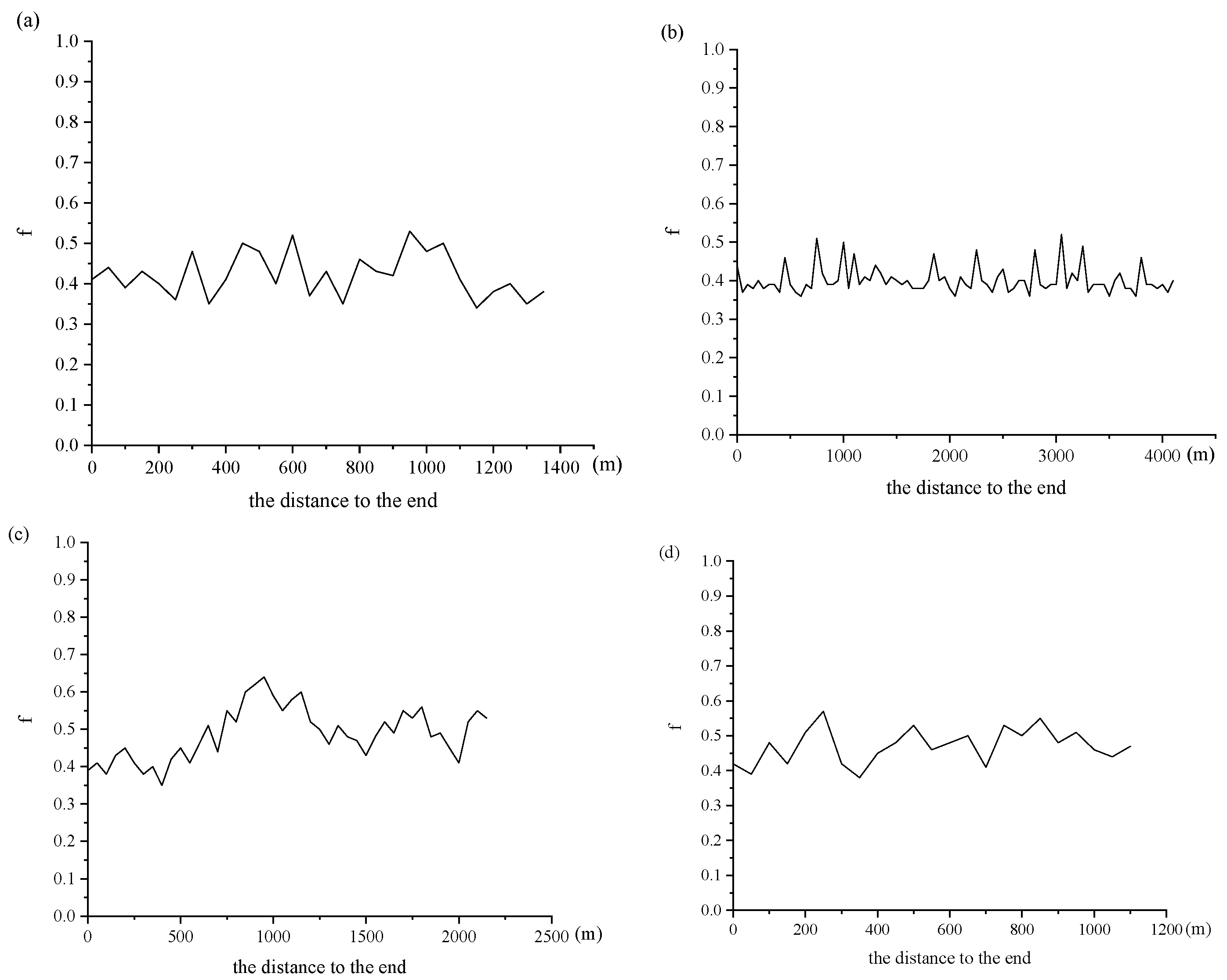
Following the method outlined in Section 3.1, recovering the valley indices of four typical glacial valleys in the Tianchi area was conducted using the GlaRe tool https://github.com/cageo/pellitero-2015 (accessed on 19 December 2023). The F-values of the Xipotingchechang Valley ranged from 0.34 to 0.53 (Figure 3a), with a mean value of 0.43. The F-values of the Songjianghe Valley ranged from 0.36 to 0.52 (Figure 3b), with a mean value of 0.40. The F-values of the Heifengkou Valley were in the range of 0.35~0.64 (Figure 3c), with a mean value of 0.49. And the F-values of the Erdaobaihe Valley were in the range of 0.38~0.57 (Figure 3d), with a mean value of 0.47.
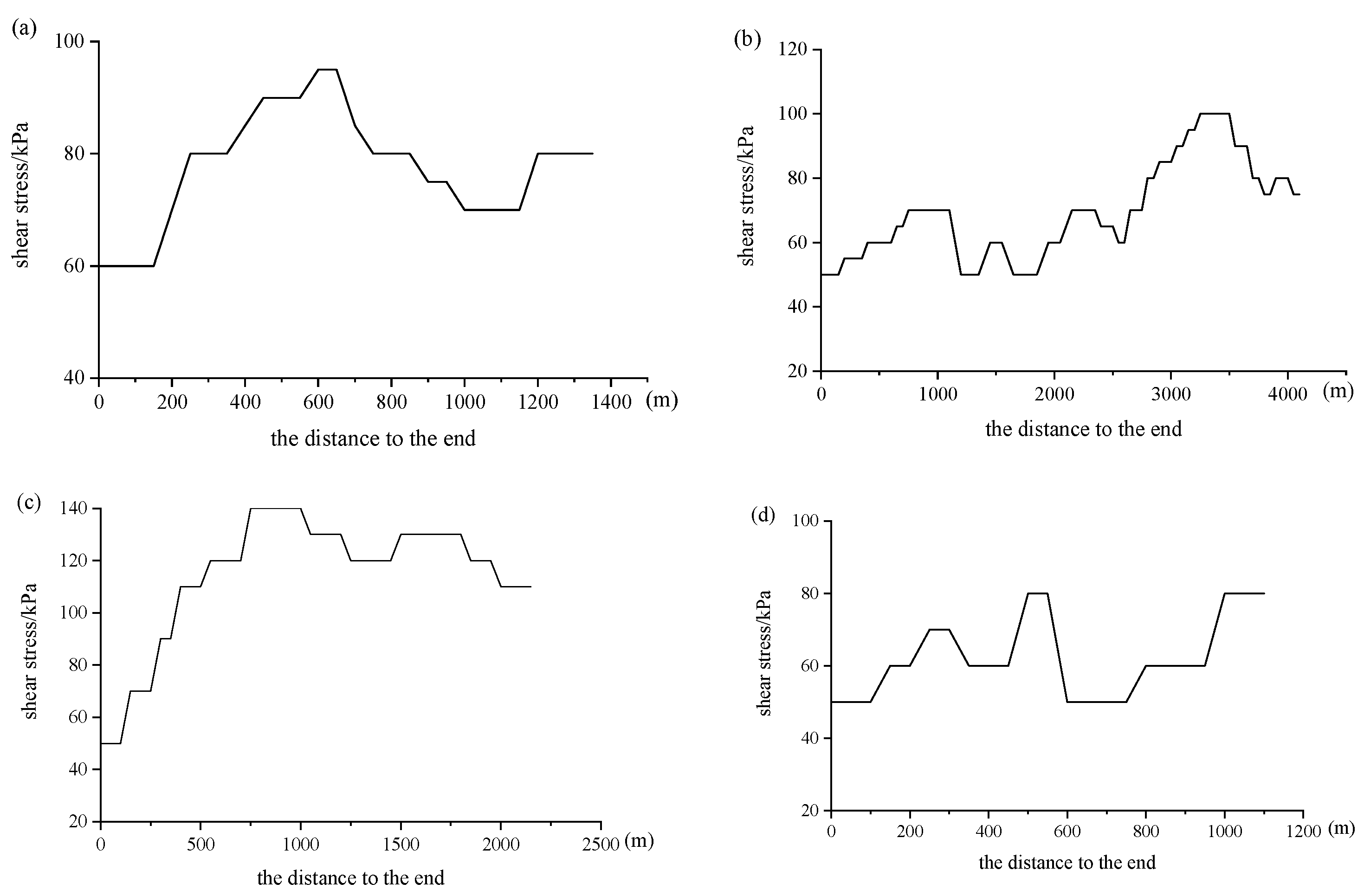
In addition, the shear stress in the Xipotingchechang Valley ranged from 60 to 95 kPa (Figure 4a), with a mean value of 77.50 kPa. In the Songjianghe Valley, the shear stress ranged from 50 to 100 kPa (Figure 4b), with a mean value of 69.15 kPa. The shear stress in the Heifengkou Valley ranged from 50 to 140 kPa (Figure 4c), with a mean value of 114.09 kPa. And the shear stress in the Erdaobaihe Valley ranged between 50 and 80 kPa (Figure 4d), with a mean value of 62.17 kPa. For valley glaciers, shear stress is usually in the range of 50~150 kPa [61]. The mean shear stress values at the bottom of each valley’s paleoglacier calculated in this study are therefore within this range.
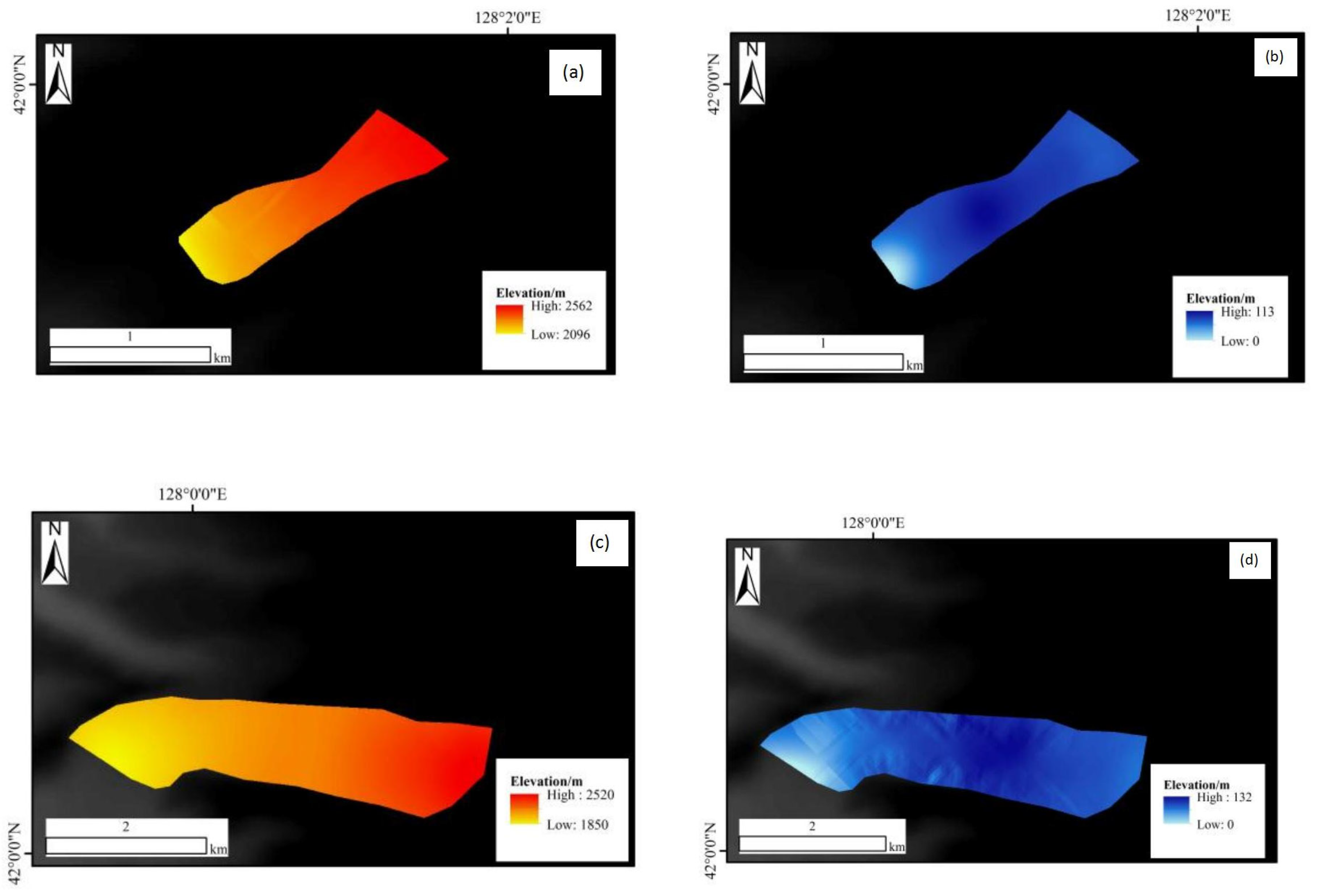
We reconstructed the paleoglacier surfaces and thicknesses of typical glacial valleys on the outer slopes of the volcanic cone of the Tianchi caldera (i.e., the Xipotingchechang, Songjianghe, Heifengkou and Erdaobaihe valleys) (Figure 5). The altitude of the paleoglacier’s surface in the Xipotingchechang Valley ranged from 2096 to 2562 m asl (Figure 4a), with a mean value of 2401 m asl. The maximum glacier thickness was calculated to have been 113 m (Figure 5b), with a mean value of 85 m. The surface area of the paleoglacier was reconstructed as 0.47 km2, and its volume was 0.04 km3. The altitude of the paleoglacier’s surface in the Songjianghe Valley ranged from 1850 to 2520 m asl (Figure 5c), with a mean value of 2195 m asl. The maximum glacier thickness was reconstructed as 132 m (Figure 5d), with a mean value of 103 m. The area of the paleoglacier’s surface was reconstructed as 3.72 km2, and its volume was 0.39 km3. The altitude of the paleoglacier’s surface in the Heifengkou Valley was in the range of 1952~2492 m asl (Figure 5e), with a mean value of 2247 m asl. The maximum glacier thickness was reconstructed as 134 m (Figure 5f), with a mean value of 84 m. The paleoglacier’s surface area shows as 0.88 km2, and the volume of the paleoglacier was 0.07 km3. The altitude of the paleoglacier’s surface in the Erdaobaihe Valley was in the range of 1856~2040 m asl (Figure 5g), with a mean value of 1967 m asl. The maximum thickness of this paleoglacier is shown to be 119 m (Figure 5h), with the mean value of 91 m. The paleoglacier’s surface area was shown to be 1.24 km2, and its volume was 0.11 km3. The results of the glacier size reconstruction revealed that the total glacial coverage of the four glacial valleys on the outer edge of the caldera was reconstructed as 6.31 km2 during the LGM, with a total volume of 0.61 km3.
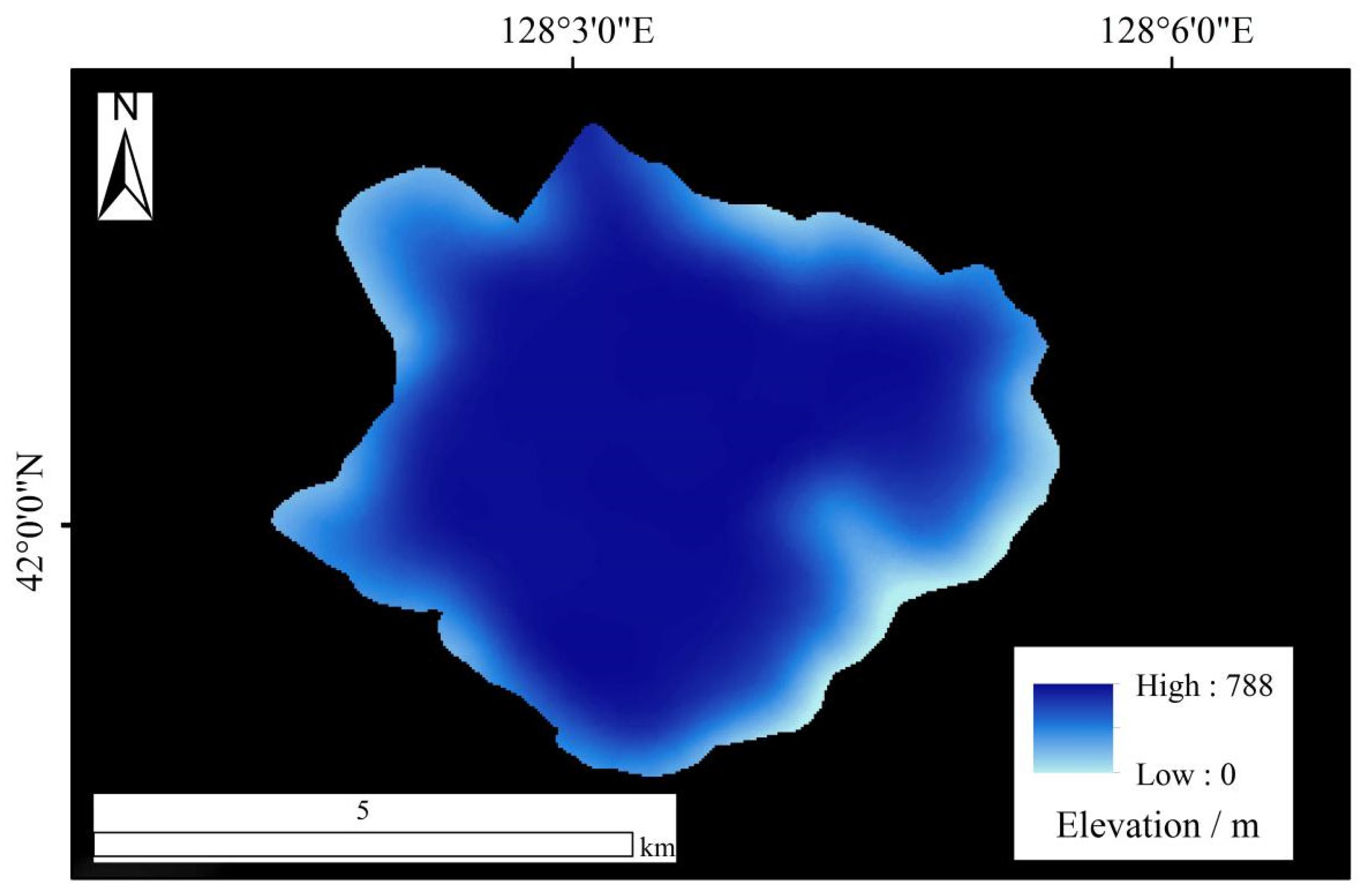
The lake volume calculation function in ArcGIS was applied to the inner crater to find out the volume of the paleoglaciers accommodated within the crater of the Tianchi Volcano during the LGM. Glacier coverage in the Tianchi caldera during the LGM period in the study area is 20.74 km2. The result shows that there is a 788 m maximum glacial thickness (Figure 6), and the volume of ice accommodated in the caldera was calculated as 9.33 km3. In summary, glacial coverage in the Tianchi area of the Changbai Mountains during the LGM was indicated as being at least 27.05 km2, with a glacial ice volume of at least 9.94 km3.

4.2. Height of Glacial ELA

4.2.1. Determining the ELAm of Modern Glaciers in the Tianchi Area

In the Tianchi area, the mean T in June–August is 6.69 °C, and the mean P is 1362.70 mm. Meteorological data for the 1979 to 2020 period have also been recorded by the Erdaobaihe Town, Huadian and Changbai meteorological stations (Table 2) (http://www.nmic.cn) (accessed on 8 October 2023), all of which are relatively close to the Tianchi area. Analyses of the meteorological data show that the temperature lapse rate in the Tianchi area between June and August is 0.62 °C/100 m (Equation (10)), and that the precipitation gradient is 35.60 mm/100 m (Equation (11)). This study selected the June–August mean air T values and MAP data from the Tianchi meteorological station and inputted them into Equation (5) to calculate the height of the modern ELAm in the study area. And then we used Equation (8) to calculate the relationship between P and air T. We found that ∆H = 616 m and that the height of the modern ELAm in the Tianchi area was 3239 m asl.
T 6 8 = 0.0062 H + 23.263 R 2 = 0.93
P a = 0.3560 H 432.01 R 2 = 0.87

4.2.2. The ELAs of Paleoglaciers during the LGM in the Tianchi Area

Combining paleoglacier size reconstruction with Equation (7), we arrived at an AAR value of 0.51. The ELAs heights were then automatically calculated by inputting the AAR value and the BR value using the ELA calculation tool developed by Pellitero et al. [37], whilst simultaneously combining this result with the ELA values obtained using the abovementioned CF, THAR and TSAM methods. The mean value of the above results was then used to obtain the ELA values during the LGM in the study area (Table 3). In addition, tectonic uplift in the region would also have had an impact on the ELA, so the amount of post-glacial tectonic uplift that had occurred needed to be taken into account when calculating the paleoglacial ELAs. Considering that the glaciers in the Tianchi area were active during the Late Pleistocene, this paper adopted an uplift rate of 1 mm/a to correct the ELA [27]. This rendered a post-LGM uplift value for the Changbai Mountains of ~20 m. After the correction for tectonic uplift, the mean ELAs in the Tianchi area during the LGM was 2289 m asl (ELAs). This gave a paleoglacial ELA 950 m (ΔELA) lower than the modern ELAm of 3239 m asl. According to study [62], ΔELA values in the eastern mountains of China during the LGM period varied between 800 and 1200 m, which is consistent with the results of this study.

4.3. Quantitative Reconstruction and Environmental Characteristics of Paleoclimate in the Tianchi Area

4.3.1. P-T Model Reconstruction

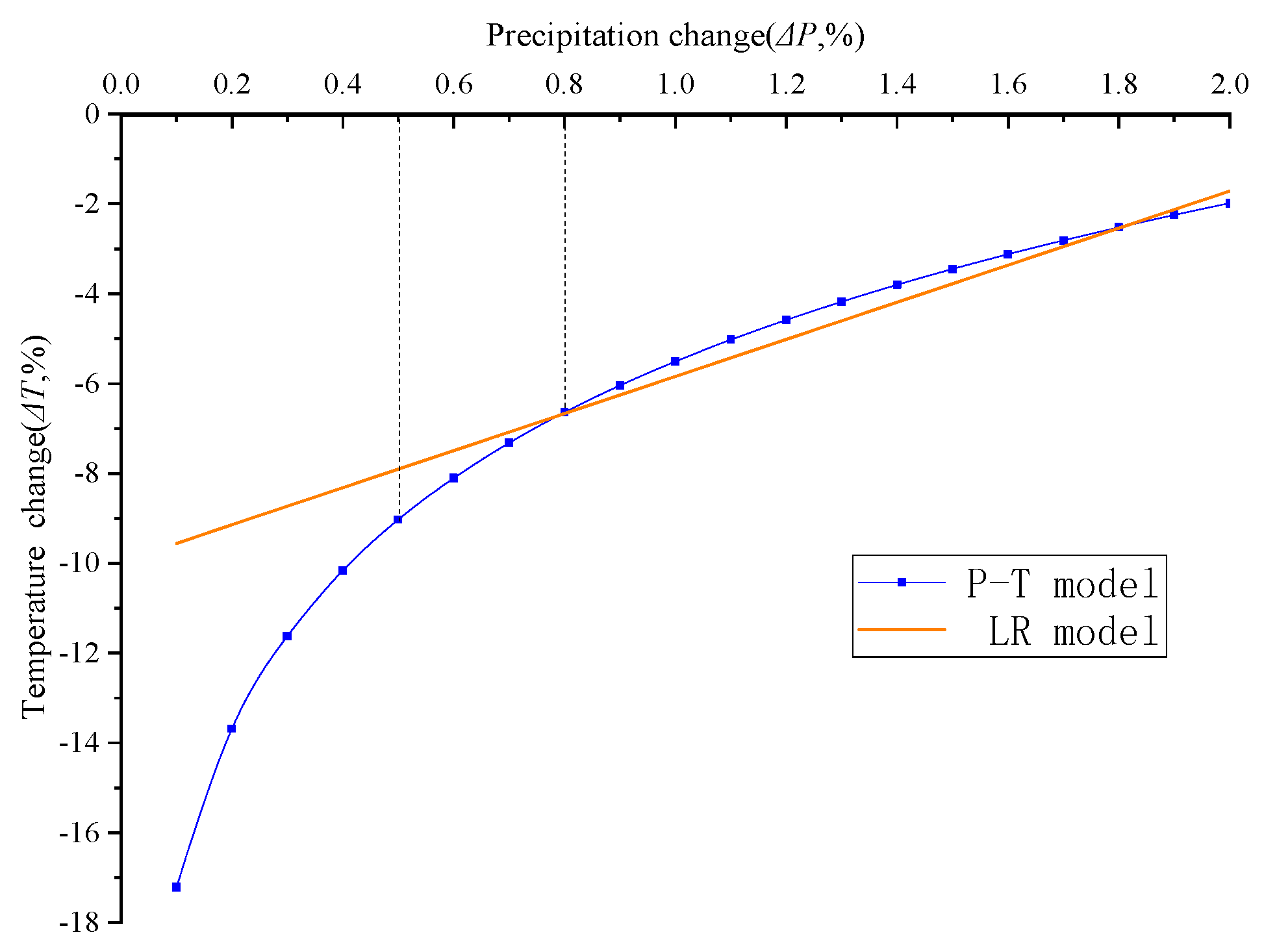
Datasets from the nearby meteorological stations showed that the temperature lapse rate is 0.58 °C/100 m in the Tianchi area and the precipitation gradient is 35.60 mm/100 m. The P at the modern ELAm was counted as 1582.20 mm and the ELA in this area fell by 950 m during the LGM (ΔELA). According to the temperature lapse rate and ΔELA of the study area, it can be inferred that the temperature in the Tianchi area during the LGM period was 5.51 °C lower than the modern temperature, i.e., the temperature change (ΔT) = −5.51 °C. It was assumed that the ratio of paleoprecipitation to modern annual precipitation at the time of glacial development in the Tianchi area represented a change from 0.1 to 2 (with modern precipitation set to 1), with a fluctuation step of 0.1. Therefore, the precipitation at the ELAs during the LGM period ranged from 158.2 to 3164.0 mm. Through the calculation of the P-T model (Equation (6)), the temperature range of the ELAs location during the LGM can be obtained as −17.1 to −1.9 °C (i.e., a mean annual temperature of −5.38 °C). Then, by adding this temperature range value to the ΔT value (−5.51 °C) derived from the temperature lapse rate, the temperature in the Tianchi area varies between −17.2 °C and −2.0 °C due to the fluctuation in precipitation during the LGM (Figure 7).

4.3.2. LR Reconstruction Results

The paleoclimatic reconstructions of the study area that employed the LR model, as opposed to the P-T model, required the following inputs: the change in T at the paleo-ELA; the change in P at the paleo-ELA; and the conversion coefficient (f) of the ELA variability vs. T during the period of glacial advance. Previous researchers have used various methods to demonstrate that the value of f lies between 2.5 × 10⁻³ and 3.3 × 10⁻³ °C/mm [63]. This study therefore chose f = 0.0029/mm °C to input into the model (Figure 7).

5. Discussion

5.1. Environmental Characteristics of the LGM in the Tianchi area

Using data analysis, Zhang [64] estimated that P during the LGP in the Changbai Mountains was ~80% of modern levels, and Shi [11] also determined that P in the Changbaishan Mountains during the LGM period was 80% of that in modern times. Based on the changes in vegetation type, Tsukada [65] deduced that P in the southwestern part of Japan, which is close to the Tianchi area, was only ~30–50% of that of the modern period during the LGM. Combined with the above research data, it can be inferred that the range of precipitation levels for the LGM in the Tianchi area was ~50–80% of modern values. The input of this data range into the P-T and LR models results in temperature ranges of −9.0 to −6.6 °C and −8.8 to −7.4 °C, respectively, so the temperature variation value is −9.0 to −6.6 °C for the Tianchi area of the Changbai Mountains during the LGM. It has been shown that the T values during the LGM in the Honshu Mountains of Japan, which are close to the Tianchi area, decreased by 7.2–7.8 °C [66], and that in the Hidaka Mountains of Japan, which have a similar latitude with the Tianchi area, decreased by 6–7 °C during the LGM [67]. Both these sets of results are comparable with this study’s findings.

5.2. Driving Factors of Glacier Development during LGM in the Tianchi Area

According to study [68], during the LGM period, the East Asian monsoon weakened and this is evidenced by the sharp decrease in the SST in the Sea of Japan and the extensive exposure of the continental shelf [69]. In addition, studies have shown that most of the northern part of China was covered by steppe during the LGM [11], and that the northeastern region was characterized by frozen desert vegetation [70]. The record from the GICC05 ice cores from Greenland [71] and from the Hulu Caveδ18O and Guliya ice core datasets also indicates a dramatic decrease in temperature during this period [58,72]. Therefore, the climate of the Tianchi area was colder and drier than it is now. Through the above analysis, it can be concluded that the main driving factor of the LGM ancient glacier advance in the Tianchi area is the decrease in temperature.

5.3. LGM Paleoclimatic Comparisons in the Monsoon Area

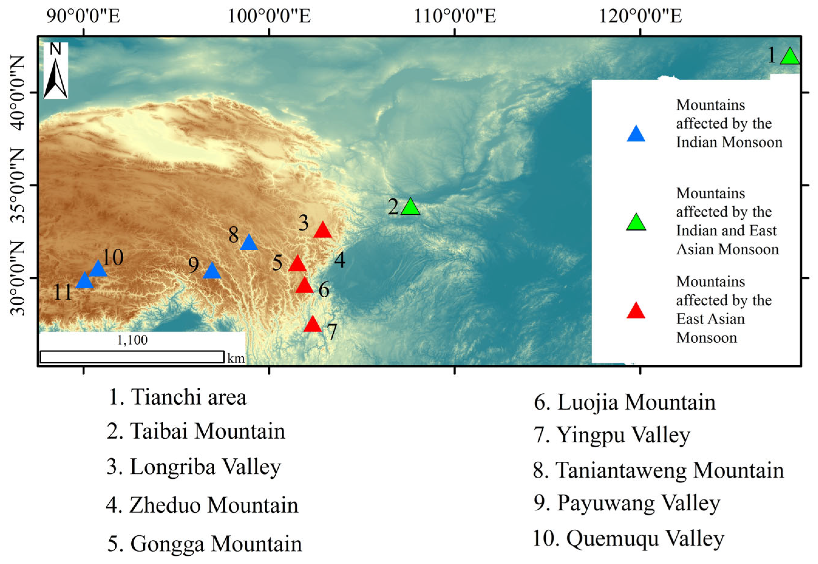
We performed a statistical analysis of mountain paleoglacial reconstruction data from monsoon-affected regions, including the East Asian monsoon and the Indian monsoon. The results show that the Tianchi area and Taibai Mountain area, which are also affected by the East Asian monsoon, have similar values of temperature decrease (Table 4), although the two mountain ranges are far apart (Figure 8). The mountain ranges located at the eastern edge of the Tibetan Plateau (Figure 8), which are both affected by the East Asian monsoon and the Indian monsoon, do not show much difference in temperature decreases (Table 4). Similarly, the mountain ranges affected by the Indian monsoon (Figure 8) also have similar values of temperature decrease (Table 4). This may indicate the similarity in the paleoclimate proxies reconstructed for the mountains affected by the same monsoon. Moreover, the temperature and precipitation variations in these mountains show that they are characterized by a cold and dry climate.
By comparing the data in Table 4, it can be seen that the temperature decrease value at the ELAs location in the mountains affected by the East Asian monsoon is more similar to that affected by both the East Asian monsoon and the Indian monsoon, while the temperature decrease value in the mountains affected by the Indian monsoon is smaller. Although these mountains are affected by monsoons, they receive less precipitation the further they are from the edge of the Tibetan Plateau. A slight decrease in temperature in the mountains with less precipitation is sufficient to balance precipitation and ablation, whereas in the mountains with more precipitation, a more substantial decrease in temperature is required to balance precipitation and ablation. This also reflects regional differences in glacier development. In terms of the variation in ELA values, the mountains that are also influenced by the Indian monsoon have smaller values for ELA variation than the others, which is also consistent with the above results on the magnitude of temperature changes. Shi [11] also showed that the value of ELA decline in western China was smaller than that in the east during the LGM because the precipitation in the east was higher than that in the west.
In summary, there is a difference in the climate change in monsoon-influenced mountains during the LGM, but this difference may be less related to the type of monsoon and more closely related to the precipitation in the mountains.

6. Conclusions

In this paper, we reconstructed the paleoglaciers and paleoclimate of the LGM in the Tianchi area of the Changbai Mountains. The results showed that the modern ELAm in the Tianchi area of the Changbai Mountains was reconstructed as 3239 m asl. The paleo-ELA for the LGM period in the study area was calculated as 2289 m asl, corresponding to a rise of 950 m since the LGM. Glacial coverage in the Tianchi caldera during the LGM period was 20.74 km2, with a maximum glacier thickness of 788 m and a glacial ice volume in the caldera of 9.33 km3. In the valleys on the Tianchi area’s outer slopes, the maximum glacial thickness in the Xipotingchechang Valley was indicated as 113 m, with a mean value of 85 m. The glacier’s surface area was computed as 0.47 km2, with a volume of 0.04 km3. The maximum glacier thickness in the Songjianghe Valley was shown to be 132 m, with a mean value of 103 m. The glacier’s surface area was shown to be 3.72 km2, with a volume of 0.39 km3. The maximum glacier thickness in the Heifengkou Valley was estimated as 134 m, with a mean value of 84 m. And 0.88 km2 represented the glacier’s surface area, with a volume of 0.07 km3. The maximum glacier thickness in the Erdaobaihe Valley was 119 m, with a mean value of 91 m. The glacier’s surface area was shown to be 1.24 km2, with a volume of 0.07 km3. After applying the P-T and LR models and combining these with existing research data, the P ratio at the time of the LGM glacial advance in the Tianchi area varied and were in the range of ~50–80% of modern levels. The air T values declined 6.6–9.0 °C. Therefore, the decrease of temperature was the main driver of glacial development in the study area during the LGM. There is a difference in the climate change in monsoon-influenced mountains during the LGM, but this difference may be less related to the type of monsoon and more closely related to the precipitation in the mountains.

Author Contributions

Conceptualization, H.Z. and W.Z.; methodology, H.Z.; software, H.Z.; validation, H.Z. and W.Z.; formal analysis, H.Z. and W.Z.; investigation, H.Z. and W.Z.; resources, H.Z.; data curation, H.Z.; writing—original draft preparation, H.Z.; writing—review and editing, H.Z. and W.Z.; visualization, H.Z.; supervision, W.Z.; project administration, W.Z.; funding acquisition, W.Z. All authors have read and agreed to the published version of the manuscript.

Funding

This research was funded by the National Natural Science Foundation of China, grant number 42071013.

Institutional Review Board Statement

Not applicable.

Informed Consent Statement

Not applicable.

Data Availability Statement

Some or all data used in the study are available from the corresponding author by request. The data are not publicly available due to privacy.

Acknowledgments

We thank the reviewers for their constructive comments, which improved the quality of the manuscript.

Conflicts of Interest

The authors declare no conflicts of interest.

References

  1. Carrivick, J.L.; Andreassen, L.M.; Nesje, A.; Yde, J.C. A reconstruction of Jostedalsbreen during the Little Ice Age and geometric changes to outlet glaciers since then. Quat. Sci. Rev. 2022, 284, 107501. [Google Scholar] [CrossRef]
  2. Soheb, M.; Ramanathan, A.; Angchuk, T.; Mandal, A.; Kumar, N.; Lotus, S. Mass-balance observation, reconstruction and sensitivity of Stok glacier, Ladakh region, India, between 1978 and 2019. J. Glaciol. 2020, 66, 627–642. [Google Scholar] [CrossRef]
  3. Paul, O.J.; Dar, R.A.; Romshoo, S.A. Paleo-glacial and paleo-equilibrium line altitude reconstruction from the Late Quaternary glacier features in the Pir Panjal Range, NW Himalayas. Quat. Int. 2022, 642, 5–16. [Google Scholar] [CrossRef]
  4. Moore, E.M.; Eaves, S.R.; Norton, K.P.; Mackintosh, A.N.; Anderson, B.M.; Dowling, L.H.; Hidy, A.J. Climate reconstructions for the Last Glacial Maximum from a simple cirque glacier in Fiordland, New Zealand. Quat. Sci. Rev. 2022, 275, 107281. [Google Scholar] [CrossRef]
  5. Bolibar, J.; Rabatel, A.; Gouttevin, I.; Galiez, C. A deep learning reconstruction of mass balance series for all glaciers in the French Alps: 1967–2015. Earth Syst. Sci. Data 2020, 12, 1973–1983. [Google Scholar] [CrossRef]
  6. Dong, G.; Yi, C.; Caffee, M. 10Be dating of boulders on moraines from the last glacial period in the Nyainqentanglha mountains, Tibet. Sci. China Earth Sci. 2013, 57, 221–231. [Google Scholar] [CrossRef]
  7. Kessler, M.; Anderson, R.; Stock, G. Modeling topographic and climatic control of east-west asymmetry in Sierra Nevada glacier length during the Last Glacial Maximum. J. Geophys. Res. Atmos. 2006, 111, F02002. [Google Scholar] [CrossRef]
  8. Plummer, M.A.; Phillips, F.M. A 2-D numerical model of snow/ice energy balance and ice flow for paleoclimatic interpretation of glacial geomorphic features. Quat. Sci. Rev. 2003, 22, 1389–1406. [Google Scholar] [CrossRef]
  9. Rowan, A.; Brocklehurst, S.; Schultz, D.; Plummer, M.; Anderson, L.; Glasser, N. Late Quaternary glacier sensitivity to temperature and precipitation distribution in the Southern Alps of New Zealand. J. Geophys. Res. Earth Surf. 2014, 119, 1064–1081. [Google Scholar] [CrossRef]
  10. Xiao, R.; Hu, J. Several characteristics of climate and geomorphology in Northeast China since the last glacial period. J. Glac. Geoc. 1988, 2, 125–134. [Google Scholar] [CrossRef]
  11. Shi, Y. Quaternary Glaciers and Environmental Issues in Eastern China, 1st ed.; Science Press: Beijing, China, 1989; pp. 271–277. [Google Scholar]
  12. Qiu, S. Research on the ancient glaciers and periglacial landforms of Changbai Mountain. Quat. Res. 1990, 2, 137–145+197–198. [Google Scholar]
  13. Zhang, W.; Liu, R.; Liu, L. The controlling factors of glaciation during the last glacial period in the East Asian monsoon affected area. Prog. Geo. 2015, 7, 871–882. [Google Scholar] [CrossRef]
  14. Pszonka, J.; Zecova, K.; Wendorff, M. Oligocene turbidite fans of the Dukla Basin: New age data from the calcareous nannofossils and paleoenvironmental conditions (Cergowa beds, Polish–Slovakian borderland). Geol. Carpath. 2019, 70, 311–324. [Google Scholar] [CrossRef]
  15. Pszonka, J.; Wendorff, M.; Godlewski, P. Sensitivity of marginal basins in recording global icehouse and regional tectonic controls on sedimentation. Example of the Cergowa Basin, (Oligocene) Outer Carpathians. Sediment. Geol. 2023, 444, 106326. [Google Scholar] [CrossRef]
  16. Wang, S.; Wen, X. The Last Glacial Maximum. Adv. Clim. Chang. Res. 2011, 5, 381–382. [Google Scholar]
  17. Cui, H.; Cao, G.; Chen, K.; Guo, H.; Jiang, G. Climates since late quaternary glacier advances: Glacier-climate modeling in the Kunlun Pass area, Burhan Budai Shan, northeastern Tibetan Plateau. Quat. Int. 2020, 553, 53–59. [Google Scholar] [CrossRef]
  18. Wang, J.; Cui, H.; Harbor, J.M.; Zheng, L.; Yao, P. Mid-MIS3 climate inferred from reconstructing the Dalijia Shan ice cap, north-eastern Tibetan Plateau. J. Quat. Sci. 2015, 30, 558–568. [Google Scholar] [CrossRef]
  19. Xu, X.; Wang, L.; Yang, J. Last Glacial Maximum climate inferences from integrated reconstruction of glacier equilibrium-line altitude for the head of the Urumqi River, Tianshan Mountains. Quat. Int. 2010, 218, 3–12. [Google Scholar] [CrossRef]
  20. Xu, X.; Yi, C. Timing and configuration of the Gongga II glaciation in the Hailuogou valley, eastern Tibetan Plateau: A glacier-climate modeling method. Quat. Int. 2017, 444, 151–156. [Google Scholar] [CrossRef]
  21. Xu, X.; Pan, B.; Dong, G.; Yi, C.; Glasser, N.F. Last Glacial climate reconstruction by exploring glacier sensitivity to climate on the southeastern slope of the western Nyaiqentanglha Shan, Tibetan Plateau. J. Glaciol. 2017, 63, 361–371. [Google Scholar] [CrossRef]
  22. Xu, X.; Yao, T.; Xu, B.; Yi, C.; Sun, Y.; Zeng, X.; Dong, G.; Pan, B. Glacial events during the last glacial termination in the Pagele valley, Qiongmu Gangri peak, southern Tibetan Plateau, and their links to oceanic and atmospheric circulation. Quat. Res. 2020, 95, 129–141. [Google Scholar] [CrossRef]
  23. Xu, X.; Yao, T.; Xu, B.; Zhang, L.; Sun, Y.; Pan, B. Last Glacial Maximum glacier modelling in the Quemuqu Valley, southern Tibetan Plateau, and its climatic implications. Boreas 2020, 49, 286–295. [Google Scholar] [CrossRef]
  24. Liu, L.; Zhang, H.; Zhang, W.; Chai, L. Global last glacial maximum climate inferred from reconstructing the eryehai valley, mount taibai, qinling mountains, eastern china. Palaeogeogr. Palaeocl. Int. J. Geo-Sci. 2022, 590, 110858. [Google Scholar] [CrossRef]
  25. Liu, J.; Wang, S. The Formation Age of Changbai Mountain Volcano and Tianchi Lake. Chin. Sci. Bull. 1982, 21, 1312–1315. [Google Scholar]
  26. Li, B. Interpretation of Aviation Satellite Photos of Glacier Landform in the Baitou Mountain Area. Geol. Rev. 1992, 5, 431–438+485–486. [Google Scholar]
  27. Zhang, W.; Niu, Y.; Yan, L.; Cui, Z.; Li, C.; Mu, K. Late Pleistocene Glaciation in the Changbai Mountains, Jilin Province. Chin. Sci. Bull. 2008, 15, 1825–1834. [Google Scholar] [CrossRef]
  28. Li, J. The remains of ancient glaciers during the last glacial period of monsoon Asia. Quat. Res. 1992, 4, 332–340. [Google Scholar]
  29. Benn, D.I.; Hulton, N.R. An ExcelTM spreadsheet program for reconstructing the surface profile of former mountain glaciers and ice cap. Comp.Geos. 2010, 36, 605–610. [Google Scholar] [CrossRef]
  30. Rea, B.R.; Evans, D.J.A. Quantifying climate and glacier mass balance in north Norway during the Younger Dryas. Palaeogeography 2007, 246, 307–330. [Google Scholar] [CrossRef]
  31. Evans, D.J.; Rea, B.R.; Hansom, J.D. Geomorphology and style of plateau icefield deglaciation in fjord terrains: The example of Troms-Finnmark, north Norway. J. Quat. Sci. 2002, 17, 221–239. [Google Scholar] [CrossRef]
  32. Locke, W.W. Modeling of icecap glaciation of the northern Rocky Mountains of Montana. Geomorphology 1995, 14, 123–130. [Google Scholar] [CrossRef]
  33. Schilling, D.H.; Hollin, J.T. Numerical reconstructions of valley glaciers and small ice caps. In The Last Great Ice Sheets; Wiley: Hoboken, NJ, USA, 1981; pp. 207–220. [Google Scholar]
  34. Nye, J. The mechanics of glacier flow. J. Glac. 1952, 2, 82–93. [Google Scholar] [CrossRef]
  35. Cuffey, K.M.; Paterson, W.S.B. The Physics of Glaciers, 4th ed.; Elsevier: Boston, MA, USA, 2010. [Google Scholar]
  36. Veen, C.J. Fundamentals of Glacier Dynamics, 2nd ed.; Balkema: Rotterdam, The Netherlands, 2013. [Google Scholar]
  37. Pellitero, R.; Rea, B.R.; Spagnolo, M.; Bakke, J.; Ivy-Ochs, S.; Frew, C.R.; Hughes, P.; Ribolini, A.; Lukas, S.; Renssen, H. GlaRe, a GIS tool to reconstruct the 3D surface of palaeoglaciers. Comput. Geosci. 2016, 94, 77–85. [Google Scholar] [CrossRef]
  38. Protin, M.; Schimmelpfennig, I.; Mugnier, J.L.; Ravanel, L.; Le Roy, M.; Deline, P.; Favier, V.; Buoncristiani, J.F.; Aumaître, G.; Bourlès, D.L.; et al. Climatic reconstruction for the Younger Dryas/Early Holocene transition and the Little Ice Age based on paleo-extents of Argentiére glacier (French Alps). Quat. Sci. Rev. 2019, 221, 105863. [Google Scholar] [CrossRef]
  39. Sun, Y.; Xu, X.; Zhang, L.; Liu, J.; Zhang, X.; Li, J.; Pan, B. Numerical reconstruction of Three Holocene Glacial Events in Qiangyong Valley, Southern Tibetan Plateau and their implication for Holocene climate changes. Water 2020, 12, 3205. [Google Scholar] [CrossRef]
  40. Shi, Y.; Huang, R.; Ren, B. Introduction to Glaciers in China, 1st ed.; Science Press: Beijing, China, 1988; p. 143. [Google Scholar]
  41. Ohmura, A.; Kasser, P.; Funk, M. Climate at the equilibrium line of glaciers. J. Glac. 1992, 38, 397–411. [Google Scholar] [CrossRef]
  42. Zhang, W.; Liu, B.; Cui, Z.; Li, Y.; Liu, L. Analysis of influencing factors on the equilibrium line of typical mountain glaciers in China. J. Geog. 2014, 07, 958–968. [Google Scholar] [CrossRef]
  43. Meierding, T.C. Late Pleistocene glacial equilibrium-line in the Colorado Front Range:A comparison of methods. Quat. Res. 1982, 18, 289–310. [Google Scholar] [CrossRef]
  44. Manley, G. The late-glacial climate of north-west England. Geol. J. 1961, 2, 188–215. [Google Scholar] [CrossRef]
  45. Louis, H. Schneegrenze und Schneegrenzbestimmung. Geog. Tas. 1955, 55, 414–418. [Google Scholar]
  46. Meier, M.F.; Post, A.S. Recent variations in mass net budgets of glaciers in western North America. Int. Assoc. Hydrolog. Sci. 1962, 58, 63–77. [Google Scholar]
  47. Kern, Z.; László, P. Size specific steady-state accumulation-area ratio: An improvement for equilibrium-line estimation of small palaeoglaciers. Quat. Sci. Rev. 2010, 29, 2781–2787. [Google Scholar] [CrossRef]
  48. Furbish, D.J.; Andrews, J.T. The use of hypsometry to indicate long-term stability and response of valley glaciers to changes in mass transfer. J. Glac. 1984, 30, 199–211. [Google Scholar] [CrossRef]
  49. Rea, B.R. Defining modern day area-altitude balance ratios (AABRs) and their use in glacier-climate reconstructions. Quat. Sci. Rev. 2009, 28, 237–248. [Google Scholar] [CrossRef]
  50. Pellitero, R.; Rea, B.R.; Spagnolo, M.; Bakke, J.; Hughes, P.; Ivy-Ochs, S.; Lukas, S.; Ribolini, A. A GIS tool for automatic calculation of glacier equilibrium-line altitudes. Comput. Geosci. 2015, 82, 55–62. [Google Scholar] [CrossRef]
  51. Benn, D.I.; Owen, L.A.; Osmaston, H.A.; Seltzer, G.O.; Porter, S.C.; Mark, B. Reconstruction of equilibrium-line altitudes for tropical and sub-tropical glaciers. Quat. Int. 2005, 138–139, 8–21. [Google Scholar] [CrossRef]
  52. Fu, P.; Heyman, J.; Hattestrand, C.; Stroeven, A.P.; Harbor, J.M. Glacial geomorphology of the Shaluli Shan area, southeastern Tibetan Plateau. J. Maps 2012, 8, 48–55. [Google Scholar] [CrossRef]
  53. Heyman, J.; Stroeven, A.P.; Caffee, M.W.; Hattestrand, C.; Harbor, J.M.; Li, Y.; Alexanderson, H.; Zhou, L.; Hubbard, A. Palaeoglaciology of Bayan Har Shan, NE Tibetan Plateau: Exposure ages reveal a missing LGM expansion. Quat. Sci. Rev. 2011, 30, 1988–2001. [Google Scholar] [CrossRef]
  54. Zhou, S.; Wang, J.; Xu, L.; Wang, X.; Colgan, P.M.; Mickelson, D.M. Glacial advances in southeastern Tibet during late Quaternary and their implications for climatic changes. Quat. Int. 2010, 218, 58–66. [Google Scholar] [CrossRef]
  55. Bendle, J.M.; Glasser, N.F. Palaeoclimatic reconstruction from Lateglacial(Younger Dryas Chronozone)cirque glaciers in Snowdonia, North Wales. Proc. Geol. Assoc. 2012, 123, 130–145. [Google Scholar] [CrossRef]
  56. Bowerman, N.D.; Clark, D.H. Holocene glaciation of the central Sierra Nevada, California. Quat. Sci. Rev. 2011, 30, 1067–1085. [Google Scholar] [CrossRef]
  57. Ramage, J.M.; Smith, J.A.; Rodbell, D.T.; Seltzer, G. Comparing reconstructed Pleistocene equilibrium-line altitudes in the tropical Andes of central Peru. J. Quat. Sci. 2005, 20, 777–778. [Google Scholar] [CrossRef]
  58. Carr, S.; Coleman, C. An improved technique for the reconstruction of former glacier mass-balance and dynamics. Geomorphology 2007, 92, 76–90. [Google Scholar] [CrossRef]
  59. Cui, H.; Cao, G.; Chen, K.; Guo, H.; Jiang, G. A review of research on reconstructing ancient climate using glacier landforms on the Qinghai Tibet Plateau and adjacent mountainous areas. J. Glac. Geoc. 2021, 01, 254–262. [Google Scholar] [CrossRef]
  60. Seltzer, G.O. Climatic interpretation of alpine snowline variations on millennial time scales. Quat. Res. 1994, 41, 154–159. [Google Scholar] [CrossRef]
  61. Paterson, W.S.B. The sliding velocity of Athabasca Glacier, Canada. J. Glac. 1970, 9, 55–63. [Google Scholar] [CrossRef]
  62. Su, Z.; Zhao, J.; Zheng, B. Distribution and features of the glaciers’ ELAs and the decrease of ELAs during the Last Glaciation in China. J. Glaciol. Geocryol. 2014, 36, 9–19. [Google Scholar]
  63. Ohmura, A. Physical basis for the temperature-based melt-index method. J. App. Met. 2001, 40, 753–761. [Google Scholar] [CrossRef]
  64. Zhang, L. The climate recovery during the last glacial period of the Late Pleistocene in China. J. Beijing Norm. Univ. Nat. Sci. Ed. 1980, 1, 101–118. [Google Scholar]
  65. Tsukada, M. Vegetation in subtropical Formosa during the pleistocene glaciation and the Holocene. Palaeogeogr. Palaeocl. 1967, 3, 49–64. [Google Scholar] [CrossRef]
  66. Ono, Y. Last Glacial Paleoclimate Reconstructed from Glacial and Periglacial Landforns in Japan. Geog. Rev. Jap. 1984, 57, 87–100. [Google Scholar] [CrossRef]
  67. Lin, Z.; Lu, R. Interannual meridiona ldisplacement of the East Asian upper-tropospheric jet strea m in summer. Adv. Atmos. Sci. 2005, 22, 199–211. [Google Scholar] [CrossRef]
  68. Wang, Y.J.; Cheng, H.; Edwards, R.L.; An, Z.S.; Wu, J.Y.; Shen, C.C.; Dorale, A.J. A high resolution absolute dated late pleistocene monsoon record from Hulu Cave, China. Science 2001, 294, 2345–2348. [Google Scholar] [CrossRef] [PubMed]
  69. Ono, Y.; Naruse, T. Snowline elevation and eolian dust flux in the Japanese islands during isotope stages 2 and 4. Quat. Int. 1997, 37, 45–54. [Google Scholar] [CrossRef]
  70. Sun, J.; Wang, S.; Wang, Y.; Zhou, Y.; Lin, Z.; Zhang, Q. The ancient environment of the last glacial period in Northeast China. Quat. Res. 1985, 1, 82–89. [Google Scholar]
  71. Wolff, E.W.; Chappellaz, J.; Blunier, T.; Rasmussen, S.; Svensson, A. Millennial-scale variability during the last glacial: The ice core record. Quat. Sci. Rev. 2010, 29, 2828–2838. [Google Scholar] [CrossRef]
  72. Thompson, L.G.; Yao, T.D.; Davis, M.E.; Henderson, K.A.; Mosley-Thompson, E.; Lin, P.N.; Beer, J.; Synal, H.A.; Cole–Dai, J.; Bolzan, J.F. Tropical climate instability: The last glacial cycle from a Qinghai–Tibetan ice core. Science 1997, 276, 1821–1825. [Google Scholar] [CrossRef]
  73. Yang, W.; Han, Y.; Peng, X.; Ran, Z.Z.; Liu, Q.; Liu, G.N. Paleoglacial and paleoclimate reconstructions during the global last glacial maximum in the Longriba area, eastern Tibetan plateau. J. Mt. Sci. 2021, 18, 307–322. [Google Scholar] [CrossRef]
  74. Yang, Y.; Yang, W.; Li, Y.; Liu, F.; Xiao, J.; Liu, B.; Li, M.; Liu, G. Reconstruction of palaeoglaciers and palaeoclimate in Zheduo Shan, Eastern Tibetan Plateau, during the Last Glacial Maximum. Quat. Int. 2023, 673, 18–28. [Google Scholar] [CrossRef]
  75. Tang, Q.; Zhang, W.; Liu, L.; Chai, L.; Li, Y.; Zhang, L.; Sun, B.; Zhang, H. Glacier scale and paleoclimate reconstruction since penultimate glaciation in the Qingshui Valley, Luoji mountain, western sichuan. J. Glaciol. Geocryol. 2021, 43, 1–12. [Google Scholar]
  76. Xu, X. Climates during Late Quaternary glacier advances: Glacier-climate modeling in the Yingpu Valley, eastern Tibetan Plateau. Quat. Sci. Rev. 2014, 101, 18–27. [Google Scholar] [CrossRef]
  77. Xu, X.; Glasser, N.F. Glacier sensitivity to equilibrium line altitude and reconstruction for the Last Glacial cycle: Glacier modelingin the Payuwang Valley, western Nyaiqentanggulha Shan, Tibetan Plateau. Palaeogeogr. Palaeocl. 2015, 440, 614–620. [Google Scholar] [CrossRef]
Figure 1. Location map of study area. This picture shows the location of Tianchi Lake, the location of the weather station used later and the nearby river (30 m resolution ASTER GDEM V2 dataset: http://www.gscloud.cn/) (accessed on 10 January 2024).
Applsci 14 03019 g001
Figure 2. Glacier geomorphology map of the last glacial maximum in Tianchi area of Changbai Mountains. The information in this image includes the location of the cirque, the glacier valley and the moraine in the Tianchi area (30 m resolution ASTER GDEM V2 dataset: http://www.gscloud.cn/) (accessed 19 December 2023).
Applsci 14 03019 g002
Figure 3. The F-values of four typical glacial valleys. The figure shows the specific values and changes in the F-values from upstream to downstream for different valleys. (a) Xipotingchechang Valley, (b) Songjianghe Valley, (c) Heifengkou Valley, (d) Erdaobaihe Valley.
Applsci 14 03019 g003
Figure 4. The shear stress of four typical glacial valleys. The figure shows the specific values and changes in shear stress in different valleys from upstream to downstream. (a) Xipotingchechang Valley, (b) Songjianghe Valley, (c) Heifengkou Valley, (d) Erdaobaihe Valley.
Applsci 14 03019 g004
Figure 5. This figure shows the reconstruction results of glacier size in different typical glacier valleys, including glacier thickness information and glacier surface elevation information during LGM. (a) Xipotingchechang Valley ice elevation, (b) Xipotingchechang Valley ice surface elevation, (c) Songjianghe Valley ice elevation, (d) Songjianghe Valley ice surface elevation, (e) Heifengkou Valley ice elevation, (f) Heifengkou Valley ice surface elevation, (g) Erdaobaihe Valley ice elevation, (h) Erdaobaihe Valley ice surface elevation.
Applsci 14 03019 g005aApplsci 14 03019 g005b
Figure 6. The thickness of glacier in Tianchi crater is reconstructed during the LGM.
Applsci 14 03019 g006
Figure 7. Simulation results of P-T model and LR model. The dashed line shows the proportion of precipitation in the Tianchi area during the LGM to the modern period. According to the calculation results of P-T model and LR model, the corresponding temperature change can be obtained by knowing the proportion of precipitation. The dashed line represents the precipitation ratio in the Tianchi area during LGM.
Applsci 14 03019 g007
Figure 8. Location map of selected mountains. The figure shows 10 mountains, of which the green ones are affected by the East Asian monsoon, the red ones by the combined influence of the East Asian monsoon and the Indian monsoon, and the blue ones by the Indian monsoon.
Applsci 14 03019 g008
Table 1. The bottom elevation values of 8 cirques in Tianchi crater. These data can help calculate the the equilibrium line altitude (ELA) value of the LGM.
Cirque
Name
12345678Mean Value
elevation
(m)
224322512237225222462257221922032239
Table 2. Location information of meteorological stations near Tianchi area.
Meteorological StationLongitude (°N)Latitude (°E)AltitudeTime Span
Tianchi meteorological station128.0542.0126231979–2020
Erdao meteorological station128.0742.25721.41979–2020
Changbai meteorological station128.1141.25777.81979–2020
Huadian
meteorological station
126.4542.59264.81979–2020
Table 3. ELA reconstruction during the LGM in Tianchi area. The data in this table show the results of ELA reconstruction in the study area using different methods in this paper. By averaging these results and removing the change in mountain height caused by tectonic uplift, ELA values during the LGM in Tianchi area are obtained.
Ice AgeTectonic Correction Value (m)CFTSAMTHARAARAABRCorrected Mean/m
LGM20223923742317232422932289
Table 4. Statistical data table for selected mountains. The data in this table show the changes of the ELA, the temperature and the precipitation in the mountains from modern to LGM.
Study Site∆ELA (m)
(Relative to the
Modern ELA)
Temperature
Decrease (°C)
Precipitation
Relative to
Modern
Value (%)
References
Tianchi area9506.6–9.250–80This study
Taibai Mountain14507.0–9.460–80Liu et al. [22]
Longriba Valley7256.0–7.030Yang et al. [73]
Zheduo Mountain5353.0–5.015Yang et al. [74]
Gongga Mountain7505.3–7.230–70Xu and Yi [18]
Luoji Mountain9204.0–8.060–80Tang et al. [75]
Yingpu Valley5004.0–5.940–80Xu [76]
Taniantaweng Mountain2363.5–5.010–50Sun et al. [39]
Payuwang Valley3403.3–4.430–70Xu and Glasser [77]
Quemuqu Valley3803.1–4.330–70Xu et al. [21]
Disclaimer/Publisher’s Note: The statements, opinions and data contained in all publications are solely those of the individual author(s) and contributor(s) and not of MDPI and/or the editor(s). MDPI and/or the editor(s) disclaim responsibility for any injury to people or property resulting from any ideas, methods, instructions or products referred to in the content.