Clustering Method for Signals in the Wideband RF Spectrum Using Semi-Supervised Deep Contrastive Learning

Abstract

This paper presents the application of self-supervised deep contrastive learning in clustering signals detected in the wideband RF spectrum, presented in the form of spectrograms. Radio clustering is a method of searching for similar signals within the analyzed part of the radio spectrum. Typically, it is based on one or several specific parameters processed from the signal in a given channel. The authors propose a slightly different, innovative approach; thanks to the self-supervised learning of neural networks, there is no need to define specific parameters, and the feature vector, enabling comparison of Euclidean distances between signals, is generated by a deep neural network trained using a contrastive loss function on a dataset containing different radio modulations. The authors describe self-supervised solutions based on contrastive learning and the methods of signal segmentation and augmentation. The training process utilizes a custom database and the Resnet-50 network with a contrastive cost function. Radio clustering is used for autonomous spectrum analysis across wide frequency ranges and enables, among other things, the detection of tactical radio stations operating with widely dispersed frequency-hopping or a significant reduction in computational power required for real-time analysis of a large number of radio signals.

1. Introduction

The analysis of RF signals in the wideband radio spectrum is particularly crucial in cognitive radio solutions [1], spectrum monitoring [2], signal intelligence (SIGINT [3]), electronic warfare, and next-generation telecommunications network solutions. Such an analysis can be performed at various stages of radio signal processing, such as in the baseband before demodulation, after demodulation, or even in the carrier frequency domain as a slice of the wideband radio spectrum.

The radio spectrum contains wideband and narrowband signals, analog and digital signals, and continuous and pulsed signals, with modulations of amplitude, phase, and frequency, as well as their combinations. New multiplexing and channel access techniques are employed, such as orthogonal frequency-division multiplexing (OFDM), non-orthogonal multiple access (NOMA) [4,5], or spectrum spreading using pseudorandom sequences (CDMA or FHSS). The methods of phase drift correction are also widely used to improve the quality of transmission [6,7]. As a result, the range of analysis that can be applied to radio signals is highly diverse and may include detecting the modulation used, searching for specific synchronization sequences, observing band occupancy over time (PSD), and more.

Modern radio receivers, measurement receivers, and spectrum analyzers are often built based on software-defined radio (SDR) architecture. SDR technology was defined by IEEE 1900.1 [8] as a radio in which some or all functions of the physical layer are defined by software. The undeniable advantage of a software-defined radio is its reconfigurability, allowing for changes in the parameters of the received or transmitted signal, not only statically but also dynamically, depending on the radio conditions. Furthermore, with increasing challenges in managing radio spectrum occupancy, there is a growing demand for cognitive and intelligent radio station solutions that rely on SDR and machine learning elements.

The article explores the use of radio spectrograms in machine learning, specifically in the radio signal clustering present in spectrograms, using deep neural networks.

2. The Signal Clustering Idea in a Radio Spectrogram

Typically, in signal analysis for a single radio channel, various classification methods, including accurate or heuristic algorithms, can be successfully applied, such as those operating on a radio spectrogram. However, the challenge remains to develop solutions that can analyze signals in real time in the wideband radio spectrum, including those that can simultaneously analyze multiple detected signals (sometimes dozens to hundreds) within the analyzed bandwidth. Therefore, there is a need for the preliminary selection of radio signals that are of interest from the perspective of a specific scenario of a wideband cognitive spectrum analyzer operation.

The clustering of radio signals in the wideband spectrum is a process aimed at distinguishing signals with similar characteristics, such as received power, modulation, bandwidth, duration, the same radio fingerprint [9,10,11], or originating from the same direction. One of the fundamental tasks requiring a preclassifier is the detection of signals from an anti-eavesdropping and jamming countermeasures radio station through the use of frequency-hopping spread spectrum (FHSS) spectrum spreading.

Examples of goals for the clustering of FHSS signals include the need for the autonomous determination of specific hopping frequencies, examining the vulnerability of TRANSEC (TRANsmission SECurity) measures, and autonomously avoiding collisions or jamming through real-time spectrum monitoring.

In typical signal clustering solutions, Key Indicators (KIs) are utilized, which are specific metrics based on which signals can be compared to each other and then assigned to specific groups. However, this requires the development of these indicators and often the application of complex algorithms that analyze at least several parameters of the radio signal. In this article, we present a different, innovative semi-supervised method for clustering radio signals in the wideband spectrum, which does not require defining KIs for this purpose.

3. Clustering Process

The first step in the preclassification and clustering process of signals in a radio spectrogram is signal detection using a method that ensures high true positive detection probability, while minimizing the false positive detection probability. In narrowband spectrum sensing solutions, various signal detection methods are typically employed, such as the energy detector, cyclostationary detector, matched filter, correlation detector, or wavelet detector. 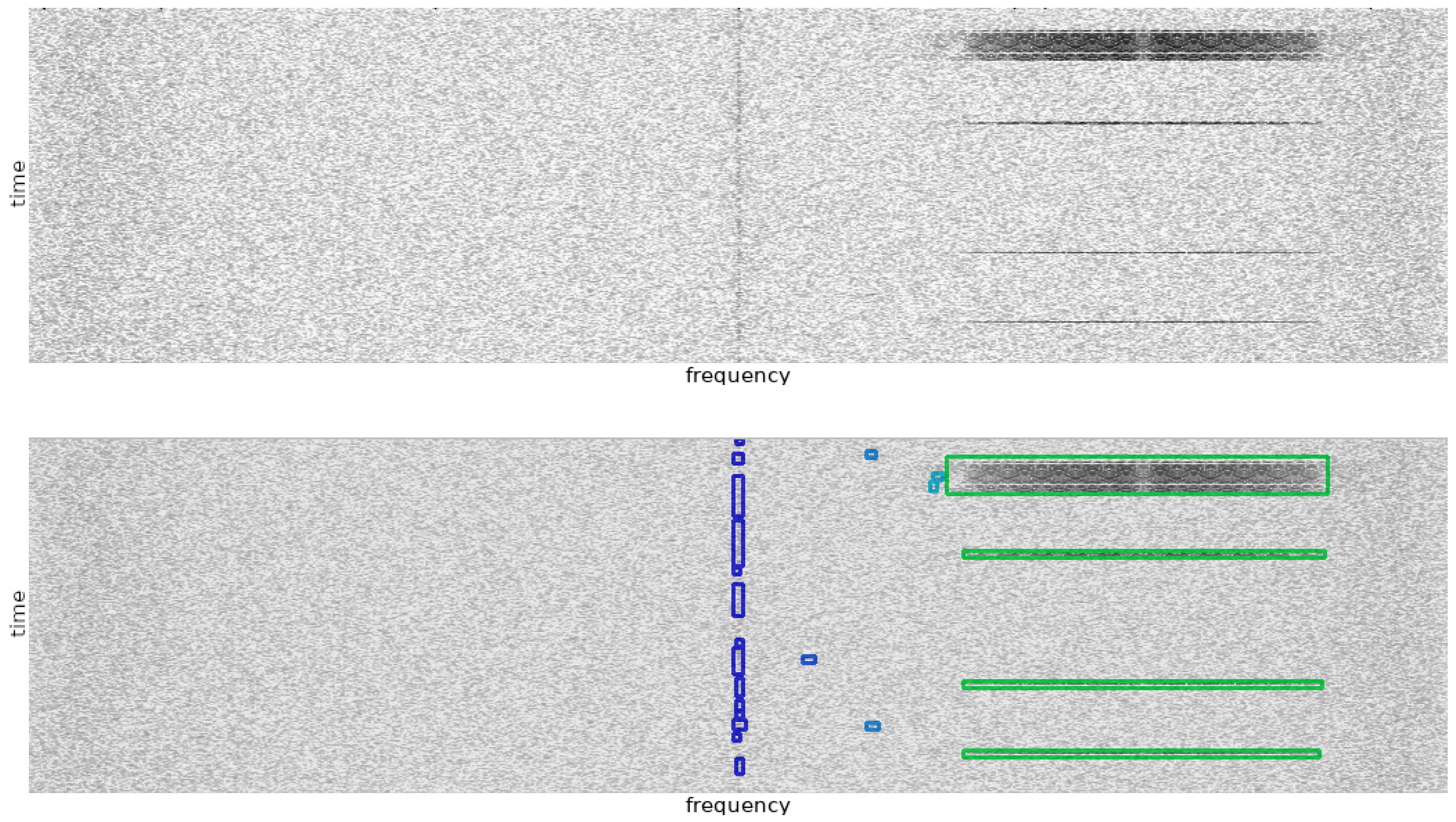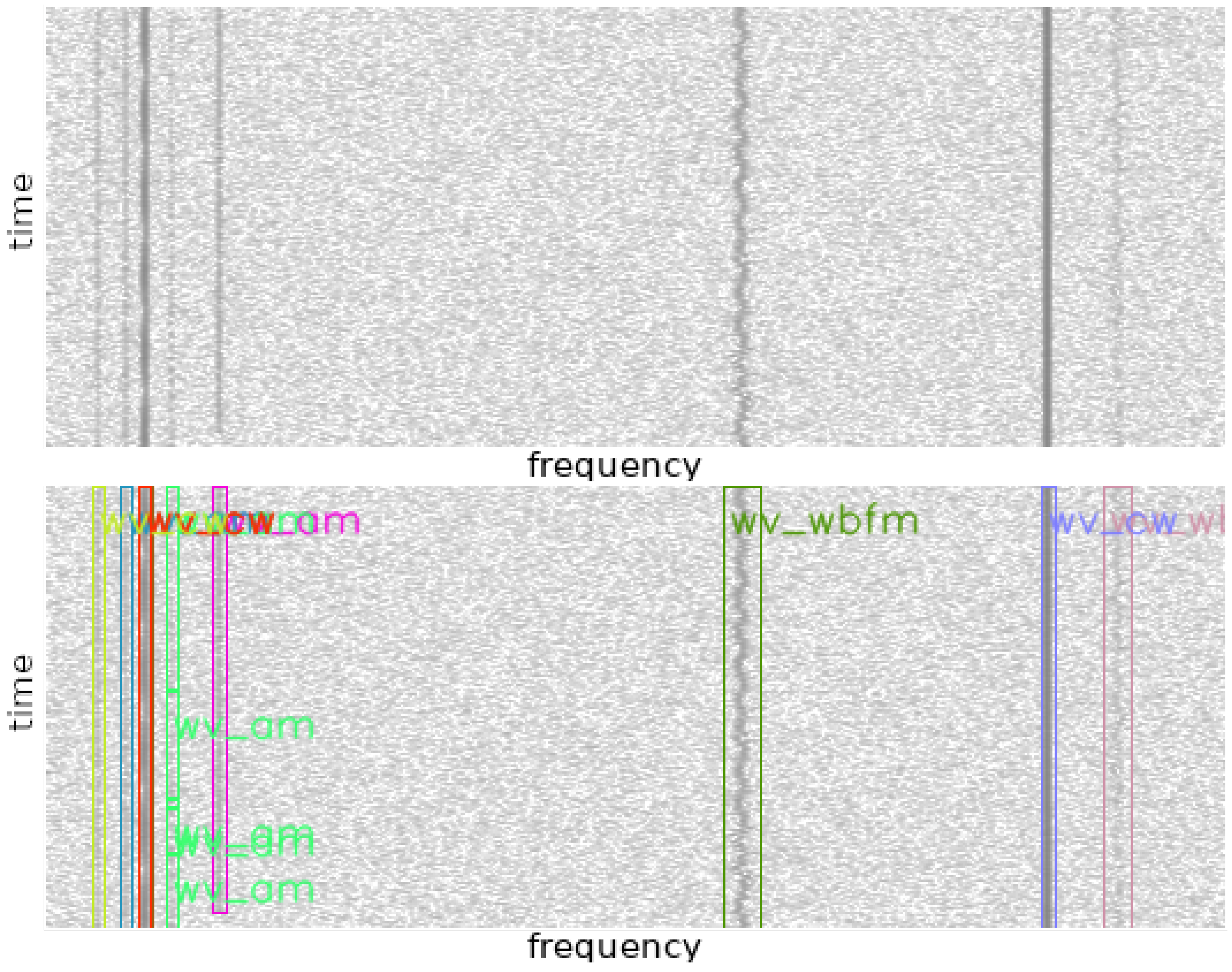However, in the case of wideband analysis and unknown signal characteristics in the spectrum, the set of possible detectors narrows down to the energy detector (ED [12,13,14]) or its extensions (e.g., ED-ENP [14]), including convolutional neural network-based detectors such as RFROI-CNN [15]. These methods enable the identification of regions of interest in the wideband spectrum, even at low signal-to-noise ratio (SNR) values. An example spectrum with detected radio signals by a convolutional detector is shown in Figure 1.

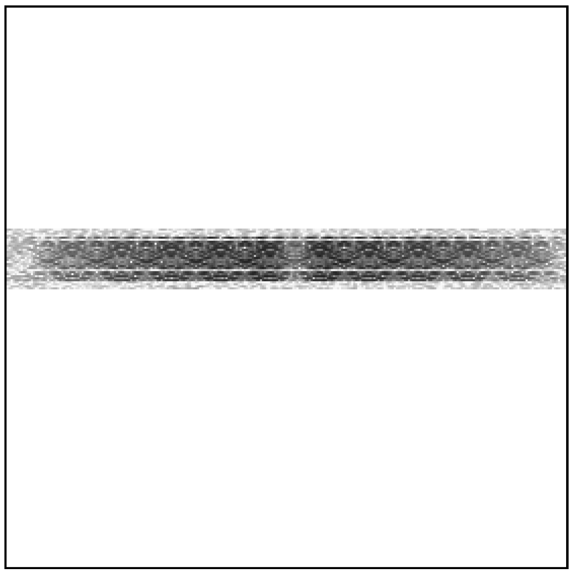
The selected regions are a list of attributes for the signal extractor module and consist of four time-frequency coordinates $[x_{min},y_{min},x_{max},y_{max}]$, where x carries frequency information and y carries time information, and around which a useful radio signal is likely to be present. The signal extractor’s task is to extract a subtensor of the size determined by the coordinate list, containing a single signal along with channel noise. An example extraction of a wideband signal from Figure 1 is shown in Figure 2.

To perform clustering, a universal method of signal representation in the form of a feature vector is required. Such a vector can be obtained from a properly trained convolutional neural network. Commonly used feature extractors are autoencoder networks [16], which consist of an encoder and a decoder. They are trained in such a way that the output tensor generated from the latent vector is as similar as possible to the input tensor.

When a tensor (e.g., an image or spectrogram) is passed into a trained autoencoder model, a feature vector is generated. If the goal is to compare multiple tensors for similarity, one can simply calculate the Euclidean distances between the feature vectors of the respective tensors. However, in the case of unsupervised learning, a problem arises when two images depicting completely different objects are not necessarily far apart in the latent space. Instead, they may concentrate within a narrow region of that space. One compromise solution to this problem is to introduce supervised learning, which allows maximizing the distances between feature vectors of tensors with different labels.

From the experiments conducted by authors during preliminary research on the application of deep neural networks in the RF environment, it is evident that the use of unsupervised learning powered by conventional autoencoders with MSE or cross-entropy loss functions for clustering yields mediocre results. Not only does the proximity issue arise in the latent space, but the autoencoder network is also often unable to reconstruct the signal shape effectively, as it is typically designed for image-related tasks. This is likely due to the high randomness of radio signal data in the form of additive noise, which, considering the logarithmic power spectral density representation, can significantly impact the network training process. Moreover, the loss functions used may not be well suited for this problem. On the other hand, leveraging labels and supervised learning reduce the preclassification subsystem to a simple signal classifier trained on the signals used during the training process. However, as mentioned earlier, the electromagnetic environment is highly complex, and it is challenging to gather a diverse range of signals within a single database.

Therefore, an alternative approach is needed for training a signal preclassification network in the radio spectrogram domain without relying on labels. One such method is self-supervised learning with a contrastive loss function.

4. Contrastive Learning

Contrastive learning is based on the assumption that representations of similar data should be close to each other in the latent space, while dissimilar data should be as far apart as possible. There are several approaches to contrastive learning, but one that has gained popularity for visual representations is SimCLR (Simple Contrastive Learning of Representations) [17]. The authors of SimCLR simplified certain self-supervised contrastive learning algorithms without the need for custom network architectures.

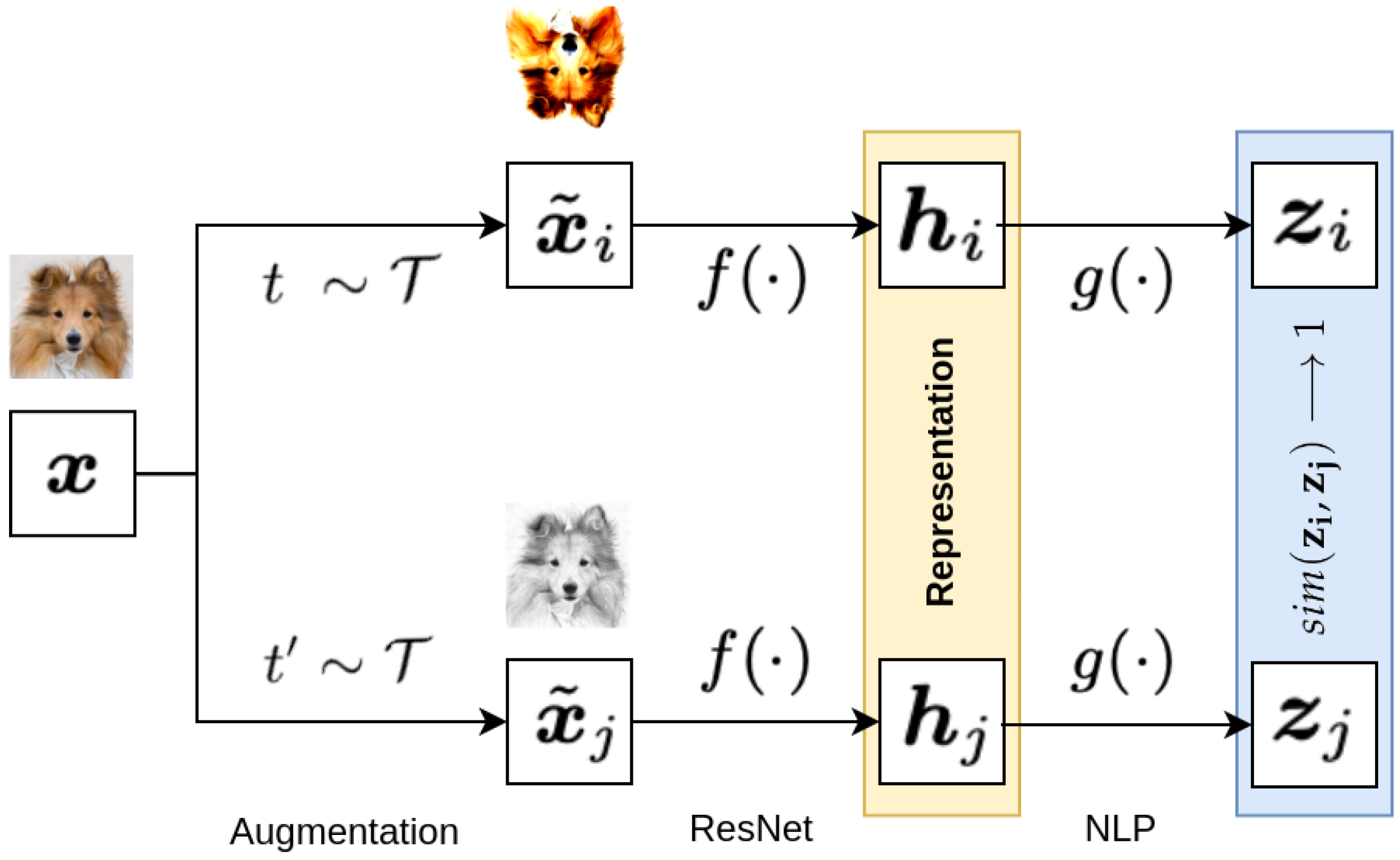
During training using contrastive methods like SimCLR [17], a positive pair is sampled from the database, which consists of two representations with the same content, or alternatively, one representation from which a positive pair is generated through appropriate transformations, as shown in Figure 3.

The input tensor in Figure 3 is denoted as x. Two different augmentation methods, t and $t^{\prime }$, selected from the set T, transform the tensor x into tensors $x_i$ and $x_j$, which are then fed into the encoder $f(.)$ in the form of a deep convolutional neural network. The output latent representations $h_i$ and $h_j$ from the encoder are passed through the dense layer $g(.)$, which maps the latent representations to a space where the contrastive loss function is computed. SimCLR [17] defines the contrastive loss function for the positive pair as “NT-Xent loss” (Normalized Temperature-Scaled Cross-Entropy Loss) described by Equation (1).

$${\mathcal{L}}_{i,j}=-log\frac{exp(sim({\mathbf{z}}_i,{\mathbf{z}}_j)/\tau )}{{\sum }_{k=1}^{2N}{\mathbb{1}}_{[k\ne i]}exp(sim({\mathbf{z}}_i,{\mathbf{z}}_k)/\tau )}$$

(1)

The similarity $sim({\mathbf{z}}_i,{\mathbf{z}}_j)$ and $sim({\mathbf{z}}_i,{\mathbf{z}}_k)$ is determined using cosine similarity, as described by Equation (2), where ${\mathbf{z}}_i$ and ${\mathbf{z}}_j$ are vectors obtained from the dense layer $g(.)$ for similar images, and ${\mathbf{z}}_i$ and ${\mathbf{z}}_k$ are vectors for dissimilar images.

$$sim(\mathbf{A},\mathbf{B})=\frac{{\sum }_{i=1}^n{A}_i{B}_i}{\sqrt{{\sum }_{i=1}^n{A}_i^2}\sqrt{{\sum }_{i=1}^n{B}_i^2}}$$

(2)

The contrastive loss function includes the indicator function ${\mathbb{1}}_{[k\ne i]}\in \{0,1\}$, evaluating to 1 if and only if $k\ne i$, as well as a parameter $\tau$, which is a tunable temperature parameter used to scale the input to the cross-entropy, directly affecting the feature distance in the latent space.

During the training of SimCLR [17], a minibatch is sampled from the database, and contrastive prediction is performed on augmented tensors, creating positive pairs. For a specific positive pair, the remaining augmented pairs are treated as negative pairs.

5. RF Signals Database and Data Augmentation

To train a network, it is necessary to have an appropriate database. In the case of addressing the problem of the simple classification of radio signals in the baseband, generating synthetic signals or using publicly available databases such as [18,19,20,21] is sufficient. However, for the clustering process, a database containing wideband representations of radio spectrograms was chosen. The proprietary rfspec-db [22] database was used, originally created for training neural networks for radio signal detection. The database was built based on implemented GNURadio software waveforms for AM, FM, LSB, USB, CW, and OFDM modulation. The generated database is publicly available and contains 391 spectrograms along with spectrograms of noise distribution and annotation files in .xml files, inspired by the VOC2007 dataset [23]. The database contains spectrograms for FFT sizes (1024, 2048, 4096, and 8192), temporal resolutions (256, 512, 1024, and 2048), durations (0.25, 0.5, 0.75, and 1.00) in seconds, sampling frequencies (2, 5, 10, 15, 20, 25, 30, 35, and 40) in MHz, and SNR values ranging from −4 dB to 12 dB. Due to the large sizes of files containing wideband radio spectrum IQ samples, only the spectrograms of these spectra are stored in the online database. A sample spectrogram from rfspec-db [22] is shown in Figure 4.

Considering that the database contains annotated files specifying the temporal frequency coordinates of specific signals along with their labels, it was decided to use them. This approach reduced the computational complexity of the training process (eliminating the need for signal detectors on spectrograms). However, it resulted in bounding boxes being centered too precisely around the signal on the spectrogram, which may lead to the incorrect functioning of the neural classifier with real signals from the radio electromagnetic environment. After extraction from the spectrum, these signals may not be properly centered relative to the central frequency of the subspectrogram. Therefore, during the process of extracting spectral fragments for network training, data augmentation in frequency, time, and amplitude needed to be considered.

The processing of the database for contrastive learning consisted of four steps: wideband spectrograms loading, signals extraction, adding to dictionary, and augmentation. The process began by loading the list containing paths to annotation files and spectrogram files. Then, the spectrogram file was loaded, and individual signals were extracted based on the annotations. These signals, along with their labels, were added to a dictionary. A copy of this prepared batch was created, which would undergo the augmentation process entirely. Augmentation was performed in time, frequency, and amplitude. Frequency augmentation involved trimming the spectrogram of the signal along the time axis from either side. Amplitude augmentation involved adding or subtracting a constant value. Time augmentation was the only operation that was applied simultaneously to two tensors from a pair. It involved sequentially extracting subtensors with variable overlap values. Dictionary pairs containing original and augmented data were passed to a method that overlays signal tensors of different dimensions onto a tensor of a fixed specified dimension, such as $[1,96,96]$. These prepared pairs underwent normalization within the range (0, 1) and were ready to generate the structure of the training database, which depended on the training strategy with a contrastive loss function.

6. CNN Training Strategy

In order to assess the feasibility of using contrastive learning for the clustering of radio signals, a training strategy was devised to differentiate signal modulations in the spectrogram. Consequently, modifications had to be made to the standard SimCLR [17] approach for training the network. Specifically, either a new implementation of the contrastive loss function needed to be developed or a method for generating the training batch had to be devised. The goal was to ensure that positive pairs corresponded to the same modulations, while negative pairs did not contain the same modulations. The decision was made to implement the latter option.

To implement the training strategy for the self-supervised learning of modulations during the preprocessing of the database, signal instances with specific modulations were grouped together. An additional augmentation step was introduced, which involved rotating the spectrogram of the signal by 90 degrees. These transformed spectrograms were also saved separately. Single-sideband modulations (LSB and USB) were grouped together due to their low spectrogram resolutions. This approach effectively created 10 separate signal subdatabases.

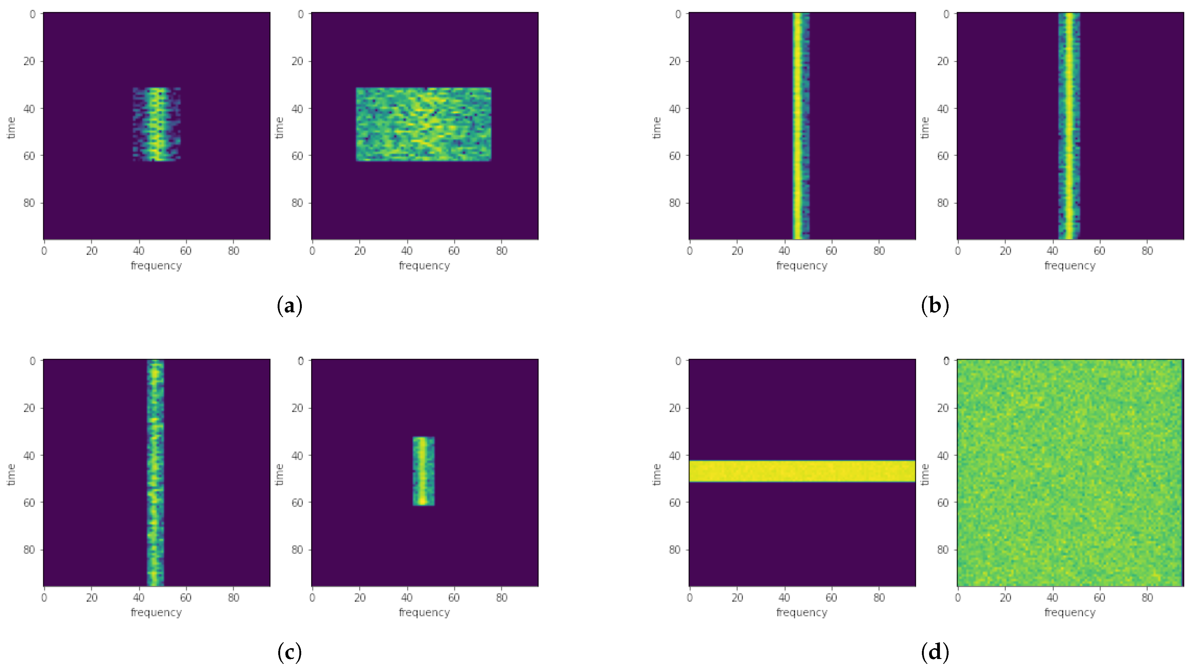
Figure 5 presents examples of positive pairs of radio signals with different SNR coefficients and various sizes of the Fourier transform. Figure 5a shows a positive pair of WBFM signals, Figure 5b shows a positive pair of AM signals, Figure 5c shows a positive pair of LSB signals, and Figure 5d shows a positive pair of OFDM signals.

Positive pairs are simultaneously negative with respect to other positive pairs. For example, a positive pair for WBFM (Figure 5a) is simultaneously negative with respect to the AM pair (Figure 5b).

The ResNet50 [24] convolutional residual network was employed as the backbone of the clustering model, with a modified dense layer that reduced the output vector size by a factor of 16, reducing from [−1, 2048] to [−1, 128]. The value 128 is a dimension of a latent vector, that is used for comparing and clustering RF signals in proposed approach. The input tensor dimensions are [3, 96, 96]. The training script used the Adam optimizer, with a learning rate set to 0.0003 and weight decay set to 1 × 10⁻⁴.

During the training process, the average loss, TOP1 accuracy, and validation clustering accuracy metrics were computed every epoch using the obtained feature vectors for the validation set. The validation set was extracted from rfspec-db [22] and consisted of the first 10% of spectrograms in the database. The Rand Index (RI) [25] was used for validation, as described by Equation (3).

$$RI=\frac{TP+TN}{TP+FP+FN+TN}$$

(3)

TP represents the number of true positives, FP represents the number of false positives, TN represents the number of true negatives, and FN represents the number of false negatives. The Rand Index takes values from 0 to 1, where 0 indicates that two sets do not agree on any pair of points, while 1 indicates that both sets are identical. We can interpret the Rand Index as a percentage measure of correct assignment decisions made by the clustering algorithm. To calculate the RI, a reference assignment of specific signals to groups (in this case, modulations) is required, obtained from the annotation files of the validation portion of the database. Subsequently, the hierarchical clustering of the obtained feature vectors for the spectrogram batch was performed using different threshold values $\lambda$ to generate assignment vectors necessary for the RI calculation.

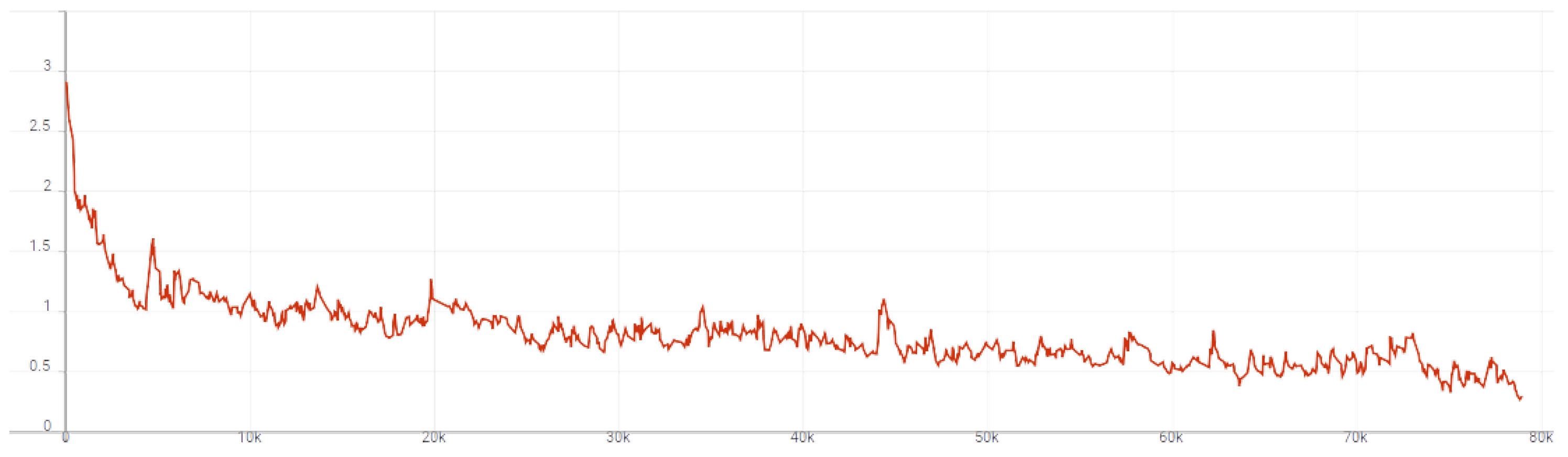
The temperature coefficient $\tau$ was initially set to 0.2. The network was trained for 50 epochs on a computer equipped with an RTX3060 GPU. The training duration for a single epoch was approximately 1 min and 23 s, resulting in a total training time of around 69 min.

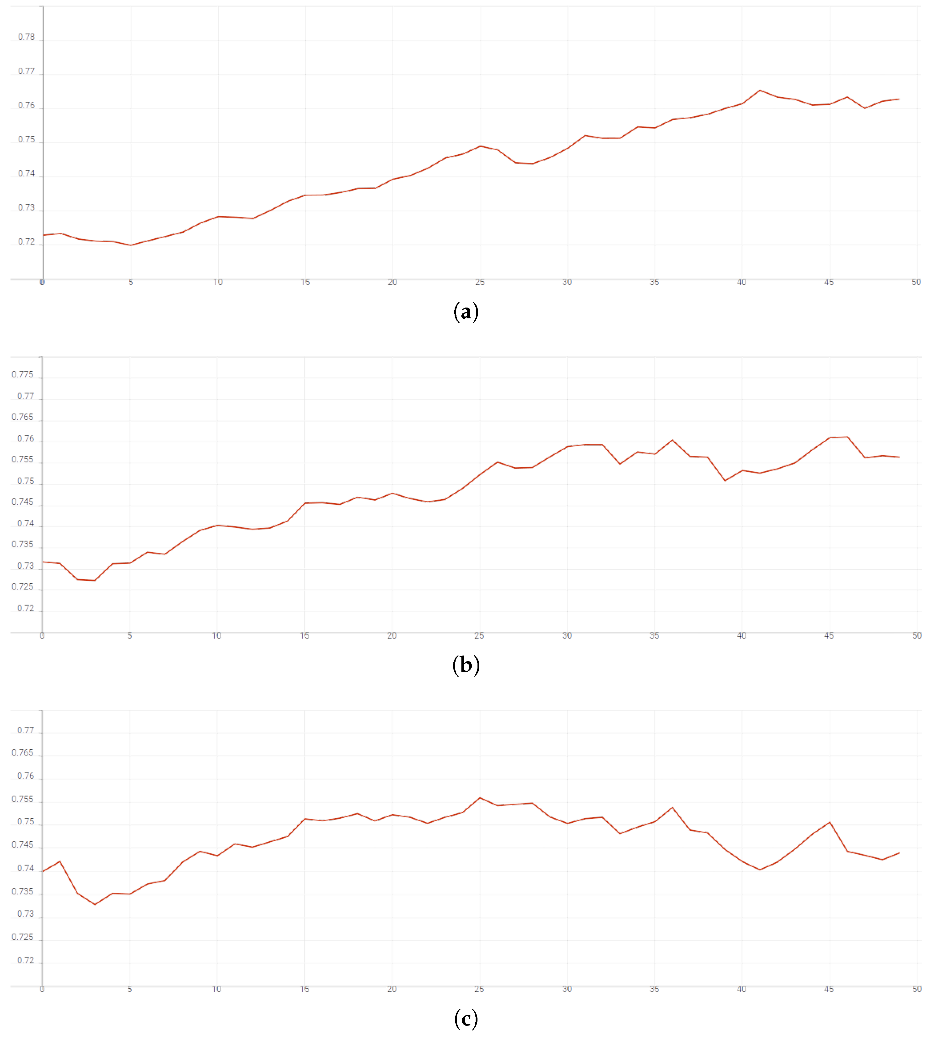
Figure 6 presents the graph of the loss function values, Figure 7a–c illustrate the Rand Index values for threshold values $\lambda$ = 5, $\lambda$ = 10, and $\lambda$ = 15, respectively. Even after 50 epochs, the accuracy_top_1 value exceeds 90%, and the Rand Index increases from the initial values of 0.73 and 0.72 for $\lambda$ = 10 and $\lambda$ = 5 to over 0.755 and 0.76, respectively.

Analyzing the Rand Index data plots, we can observe that towards the end of the DNN training (number of epochs approaching 50), the Rand index value decreases for $\lambda$ = 15, and flattens out for $\lambda$ = 10. This is due to the fact that as the training process of the neural network with a contrastive loss function progresses, similar signals tend to have lower Euclidean distances to each other. At some point, the static cutoff value at $\lambda$ = 15 or $\lambda$ = 10 becomes too high for most of the Euclidean distances determined by the trained network.

7. Evaluation of the Model and Clustering of RF Signals

Evaluating the network based on wideband radio spectrogram requires generating subspectrograms containing detected radio signals, which will be processed by the neural network. Similar to the training process, the annotation files of the rfspec-db [22] database were used, enabling the extraction of signals from the wideband spectrum without the need for energy detectors such as ED [12,13,14] or RFROI-CNN [15]. The annotation files also provide information about the modulation used, which was used for validating the proposed simple hierarchical clustering method.

The generated subspectrograms formed a batch in the form of a tensor, which was processed by the trained neural network. The output of the network was a tensor containing feature vectors of length 128 for each signal. With this set of features, we could compare signals to each other. Firstly, we needed to calculate the Euclidean distances between each pair of vectors using Formula (4).

$$d(A,B)=\sqrt{\sum _{i=1}^n{(x_{iA}-x_{iB})}^2}$$

(4)

After calculating the distance matrix, we had sufficient data to find signals that are similar in terms of modulation. We could search for the n most similar spectrograms, similar to searching for similar images, or we could define an empirically chosen threshold of Euclidean distance below which signals would be considered similar, and above which signals would be considered different from each other.

7.1. Searching for Similar RF Signals in Spectrograms

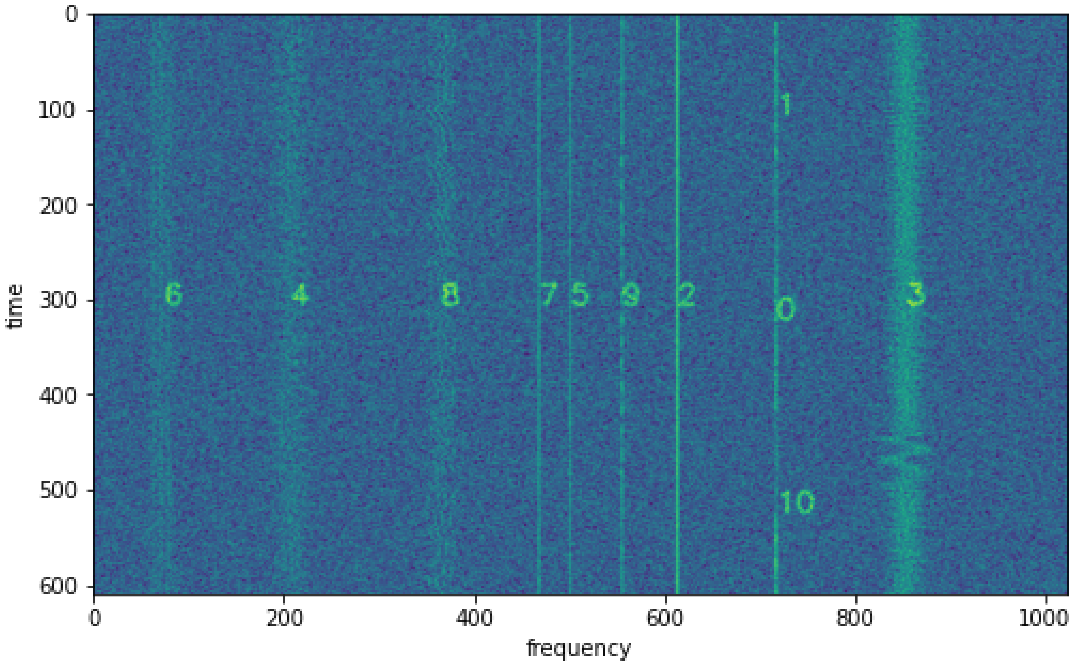
An example spectrogram, labeled in rfspec-db [22] as 000310 with signal numbers overlaid, is shown in Figure 8. Signals 0, 1, and 10 are modulated with LSB modulation, signals 2 and 5 are CW (continuous wave) carriers, signals 3, 4, 6, and 8 are FM signals, and signals 7 and 9 are AM signals. For example, to find a signal similar to signal 4 (FM signal with low SNR), we can locate the fourth row of the distance matrix, which contains the distance vector between the features of signal 4 and the other signals.

The distance vector for signal 4 is presented in Equation (5). From this vector, we can infer that the closest signal to signal 4 is signal 8 (distance of 0.84), followed by signal 6 (distance of 5.71). Signal 3 is also quite similar (distance of 10.47) compared to the subsequent signals, with the next closest signal having a distance of 31.93. All of the mentioned similar signals have the same FM modulation, while signal 3 differs from the rest in terms of its SNR indicator, exhibiting a significantly higher spectral power density in the spectrogram. Therefore, a thresholding method can be applied to extract similar signals. In order to classify signals with the same modulation and similar SNR, a threshold distance of $\lambda$ = 6 is sufficient in this case. However, to classify signals with different SNR, an optimal threshold distance value of $\lambda$ = 11 seems appropriate.

$$A_{m,4}=\left(\begin{array}{ccccccccccc}44.84& 45.30& 31.93& 10.47& 0.00& 42.51& 0.84& 41.34& 5.71& 42.37& 44.35\end{array}\right)$$

(5)

The inverted hard thresholding method (Equation (6)) for small argument values involves substituting one value (typically a logical ‘0’) for the condition greater than or equal to being met, and another value (typically, a logical ‘1’) for the condition not being met.

$$a_m\left(x\right)=\left\{\begin{array}{cc}0\hfill & \mathrm{if}\left|x\right|\ge \lambda \hfill \\ 1\hfill & \mathrm{if}\left|x\right|<\lambda \hfill \end{array}\right.$$

(6)

Therefore, after applying inverted thresholding with $\lambda$ = 6 and $\lambda$ = 11 to the distance vector from Equation (5), it will appear as shown in Equations (7) and (8), where ‘1’ indicates that the signal is similar (True) and ‘0’ indicates that the signal is dissimilar (False).

$$S_{m,4}(\lambda =6)=\left(\begin{array}{ccccccccccc}0& 0& 0& 0& 1& 0& 1& 0& 1& 0& 0\end{array}\right)$$

(7)

$$S_{m,4}(\lambda =11)=\left(\begin{array}{ccccccccccc}0& 0& 0& 1& 1& 0& 1& 0& 1& 0& 0\end{array}\right)$$

(8)

With the similarity vectors, it is possible to plot a similarity matrix, which is shown in

Table 1. Similarity of signal 4 to the other RF signals detected in the spectrogram 000310 (fft_size 1024, samp_rate 2.5 × ${10}^6$, and length = 0.5 s) from the rfspec-db database [22].

sig id	0	1	2	3	4	5	6	7	8	9	10
MOD	LSB	LSB	CW	WBFM	WBFM	CW	WBFM	AM	WBFM	AM	LSB
PSNR [dB]	16	16	11	10	4	1	1	4	2	8	16
FREQ [px]	717	717	613	852	207	500	71	468	366	555	717
4$(\lambda =6)$	False	False	False	False	True	False	True	False	True	False	False
4$(\lambda =11)$	False	False	False	True	True	False	True	False	True	False	False

for signal 4 and $\lambda$ = 6 and $\lambda$ = 11. Analyzing the table for two $\lambda$ values yields interesting conclusions. The analyzed signal 4 is modulated with WBFM. For $\lambda$ = 6, only signals 6 and 8 are considered similar, with respective PSNR values of 1 dB and 2 dB, while signal 4 has a PSNR of 4 dB. There is another WBFM radio station in the spectrogram transmitting the same modulating signal but with a higher PSNR of 10 dB. To include it in the common set for WBFM, the $\lambda$ value needs to be increased to 11. For $\lambda$ = 6 radio stations with a power difference of 3 dB are included in the set, while for $\lambda$ = 11, the power difference is 6 dB. This indicates that the trained network distinguishes not only modulations but also signal power in the spectrogram, which can be a valuable solution for recognizing signals scattered across the ultra-wideband spectrum from specific FHSS radio stations.

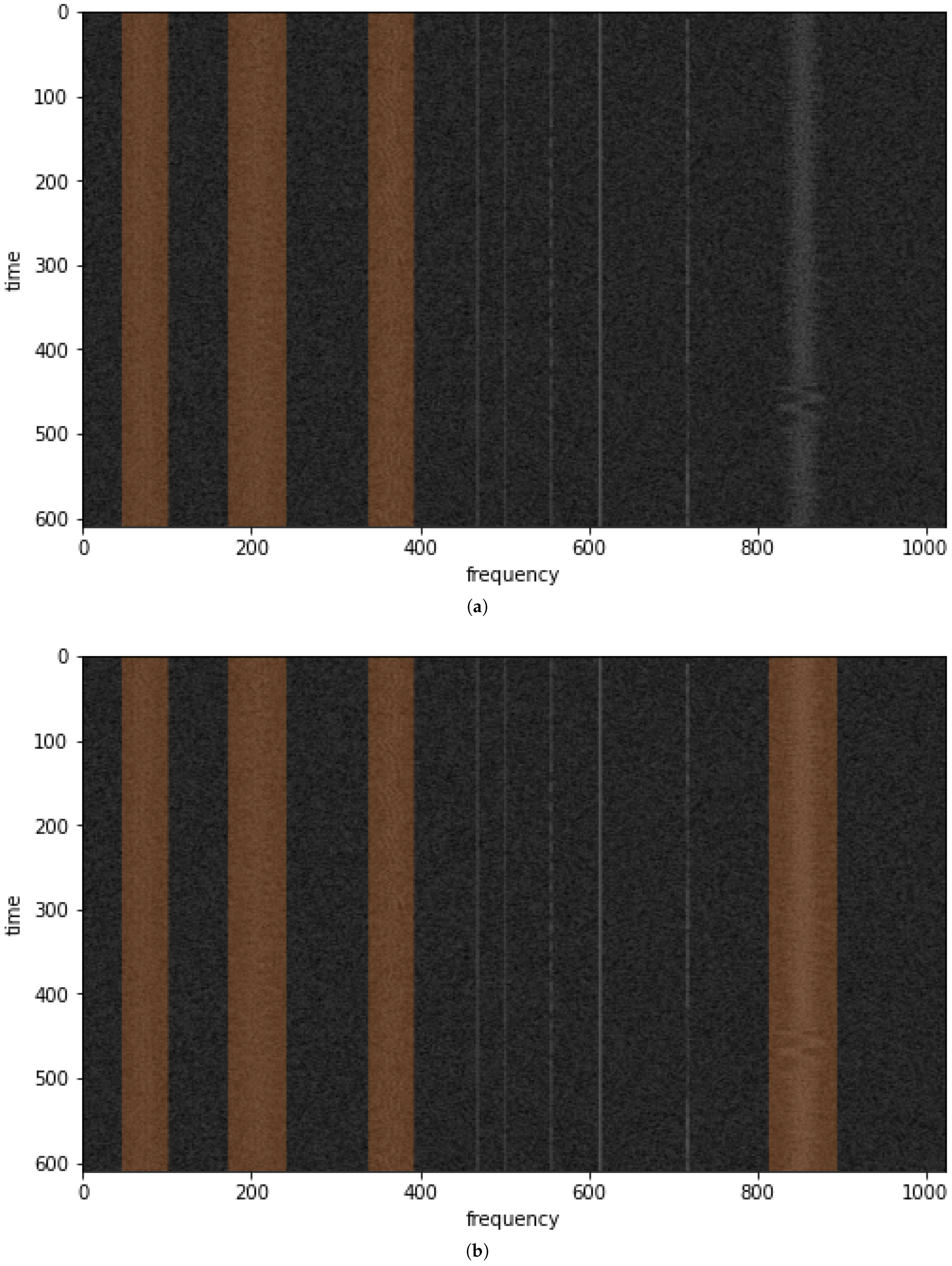
By having the similarity matrix, we can visualize the similarities between signals on the background of the wideband radio spectrogram (Figure 8), as shown in Figure 9a,b for $\lambda$ = 6 and $\lambda$ = 11, respectively. The similarities are visualized by overlaying an orange color on the detections of similar signals.

7.2. Clustering RF Signals

An interesting issue is the automatic clustering of radio signals detected and evaluated in the proposed model. We decided to evaluate the performance of clustering using hierarchical clustering, specifically agglomerative clustering [26,27].

Agglomerative clustering [26,27] is a hierarchical clustering algorithm that starts by considering each data point as an individual cluster. It iteratively merges the closest pairs of clusters based on a similarity measure until all data points belong to a single cluster. The algorithm begins by calculating the distance or similarity between each pair of data points and creates a proximity matrix. It then identifies the two closest clusters based on the proximity matrix and merges them into a new cluster. The process continues until all data points are part of a single cluster.

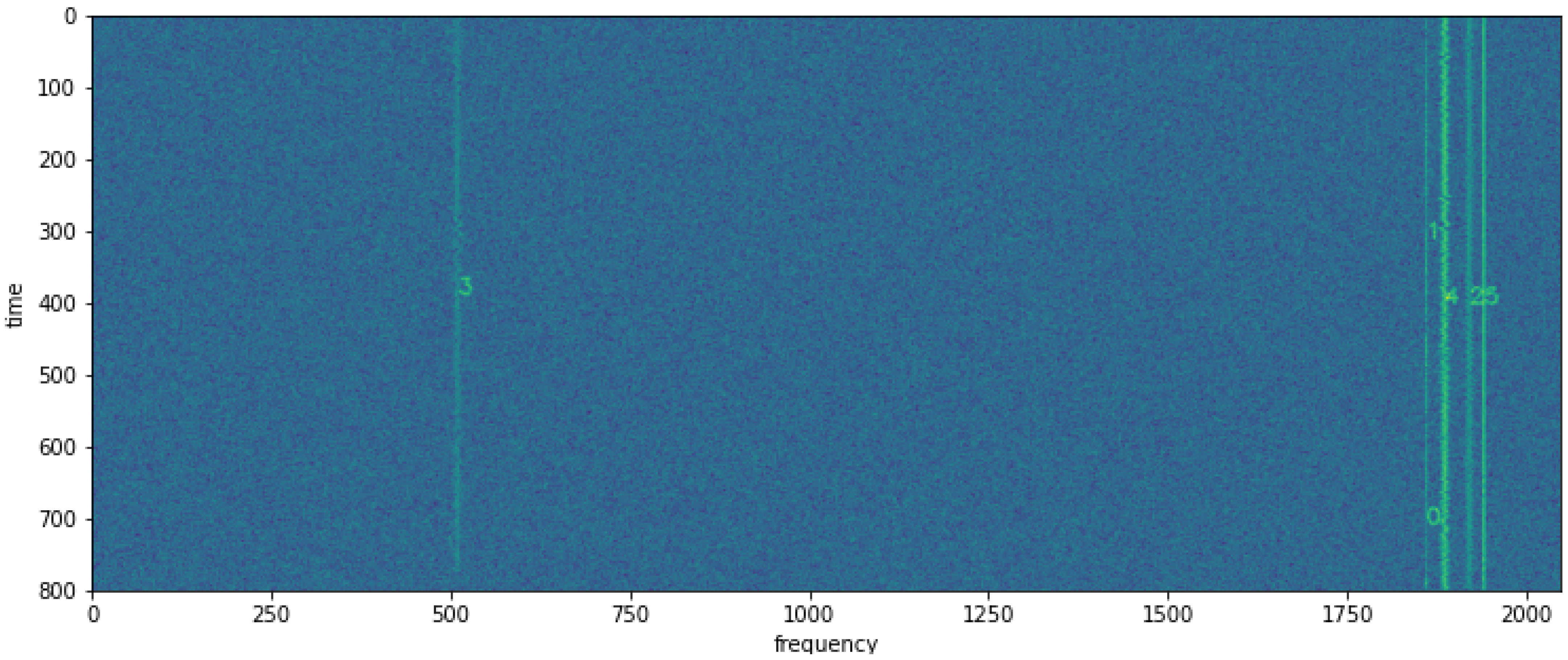
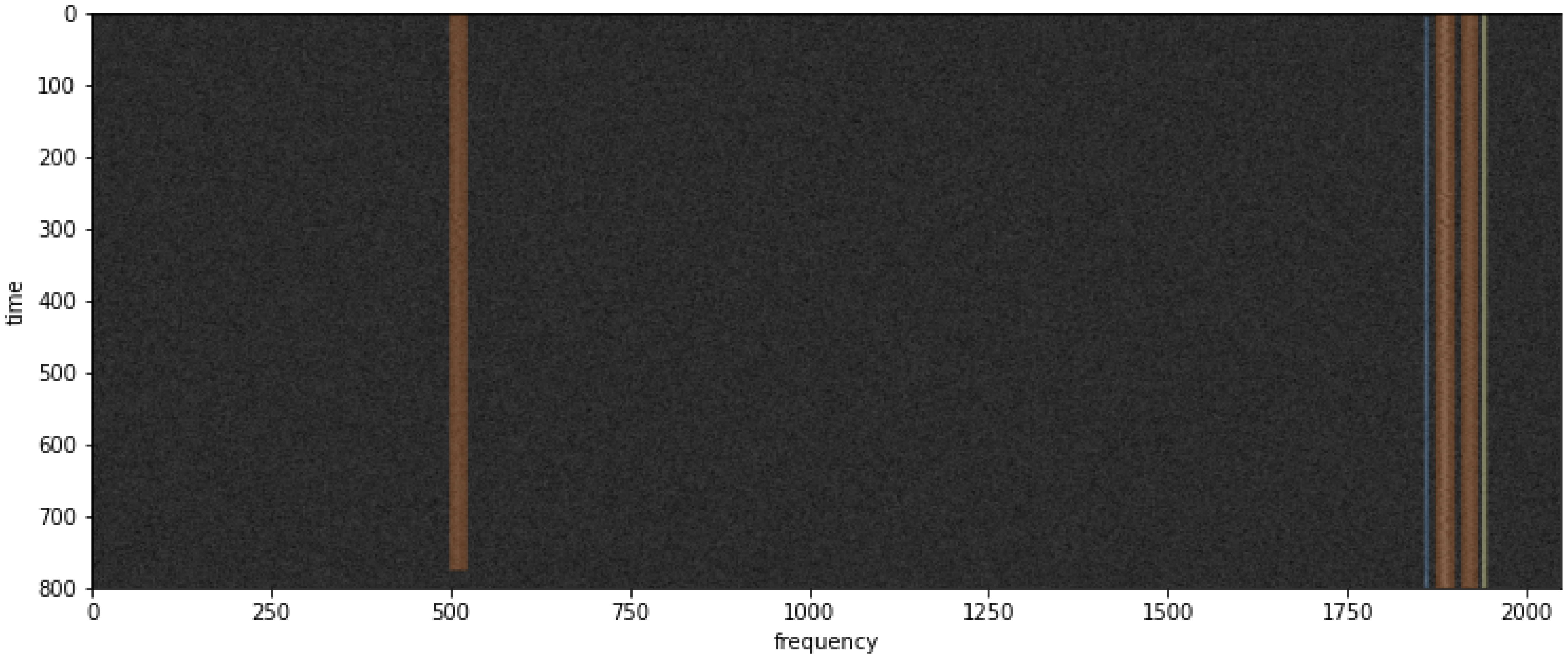
The challenge of clustering in datasets with an unknown number of clusters requires setting a threshold value $\lambda$, similar to the simple method of finding similar signals. The implementation of agglomerative clustering [26,27] was obtained from the Scikit library [28]. An example of the model’s operation, along with agglomerative clustering, is demonstrated using spectrogram 000303, which is shown in Figure 10. There are six visible signals, where 0 and 1 correspond to LSB, 2, 3, and 4 correspond to FM, and 5 corresponds to AM.

The distance matrix between signals is presented in Equation (9). With the distance matrix, the similarity matrix can be calculated as shown in

Table 2. Similarity matrix of RF signals detected in the spectrogram 000303 (fft_size 2048, samp_rate 17.5 × ${10}^6$, and length = 0.75 s) from the rfspec-db database [22].

sig id	0	1	2	3	4	5
MOD	LSB	LSB	WBFM	WBFM	WBFM	AM
PSNR [dB]	14	14	4	2	14	16
FREQ [px]	1861	1861	1920	509	1886	1942
0  $(\lambda =11)$	True	True	False	False	False	False
1  $(\lambda =11)$	True	True	False	False	False	False
2  $(\lambda =11)$	False	False	True	True	True	False
3  $(\lambda =11)$	False	False	True	True	True	False
4  $(\lambda =11)$	False	False	True	True	True	False
5  $(\lambda =11)$	False	False	False	False	False	True

. On the other hand, similar signals have been color-coded in Figure 11.

$$A_{m,n}=\left(\begin{array}{cccccc}0.00& 8.51& 36.70& 39.30& 36.27& 20.72\\ 8.51& 0.00& 32.89& 35.87& 32.48& 19.84\\ 36.70& 32.89& 0.00& 5.69& 0.90& 24.89\\ 39.30& 35.87& 5.69& 0.00& 6.46& 27.79\\ 36.27& 32.48& 0.90& 6.46& 0.00& 24.32\\ 20.72& 19.84& 24.89& 27.79& 24.32& 0.00\end{array}\right)$$

(9)

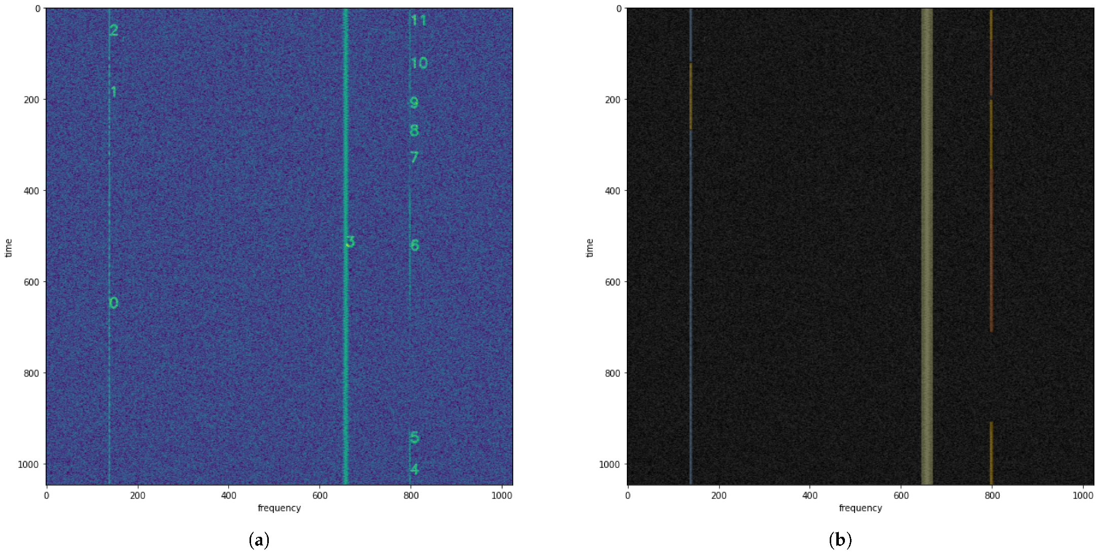
However, not all signals can be easily distinguished, as shown in the example spectrogram 000381, depicted in Figure 12a, where signals 0, 1, and 2 represent AM, signal 3 represents WBFM, and signals 4–11 represent USB. In Figure 12b, visualizations of similar signals after hierarchical clustering with an RI of 0.84 are presented.

As observed, the FM signal (3) is correctly distinguished from the others (highlighted in yellow), a portion of the AM signal (highlighted in blue) as well as the USB signals (highlighted in orange) are also correctly detected as separate signals. However, there are overlapping detections of signals 1, 11, 4, 5, 7, 8, and 9 that are not grouped with either USB or AM, even though signal 1 is actually an AM signal, and the rest are USB signals. This may be attributed to various factors. Firstly, during evaluation, only a segment of the signal with a maximum duration of 96 pixels was sampled, whereas in reality, the signal is much longer. One potential solution could be to extract all subspectrograms composing the signal and calculate the average of the latent vector. Another significant aspect is the low resolution of the spectrograms and analog modulation signals, such as in the case of SSB modulation. For instance, a long constant tone in SSB modulation on the spectrogram may appear similar to AM or CW modulation.

8. Conclusions

The paper deals with the topic of spectrum awareness, specifically the preclassification of detected signals in the wideband radio spectrum. Spectrograms were proposed as a means to apply convolutional neural networks (CNNs) in the discussed context, as the waterfall visualization depicts signal characteristics in the frequency–time–amplitude domain as a sequence of interconnected pixels, forming geometric objects easily interpretable by CNNs.

The focus of the study was on the preclassification and clustering of signals in the wideband radio spectrum. Preclassification serves the purpose of grouping similar signals and performing an initial clustering of radio signals received by a wideband receiver based on a latent feature vector generated by the network structure. An unsupervised (self-supervised) learning method was proposed, using a contrastive loss function. The approach was inspired by the SimCLR solution, but the network training strategy was modified and adapted to the problem of distinguishing signal modulations for different transform sizes, spectrogram durations, SNR coefficients, etc. An author-created database was used for training and evaluation purposes.

As part of the evaluation of the trained network model, simple searching for similar signals (based on modulation) in radio spectrograms was presented, along with the capability of automatic grouping and visualization of similar signals in the wideband radio spectrum.

The paper demonstrated the feasibility of employing deep convolutional neural networks in the analysis of wideband radio spectrum for building artificial intelligence systems operating in the domain of the radio electromagnetic environment. The preclassification of signals, exemplified in the paper using modulation as an example, can be realized for various parameters of radio signals or even radio fingerprints. This opens up new possibilities in autonomous spectral analysis, including spectrum monitoring conducted by civilian authorities or electronic warfare on the battlefield.