The Intraday Dynamics Predictor: A TrioFlow Fusion of Convolutional Layers and Gated Recurrent Units for High-Frequency Price Movement Forecasting

Abstract

This paper introduces a novel deep learning approach for intraday stock price direction prediction, motivated by the need for more accurate models to enable profitable algorithmic trading. The key problems addressed are effectively modelling complex limit order book (LOB) and order flow (OF) microstructure data and improving prediction accuracy over current state-of-the-art models. The proposed deep learning model, TrioFlow Fusion of Convolutional Layers and Gated Recurrent Units (TFF-CL-GRU), takes LOB and OF features as input and consists of convolutional layers splitting into three channels before rejoining into a Gated Recurrent Unit. Key innovations include a tailored input representation incorporating LOB and OF features across recent timestamps, a hierarchical feature-learning architecture leveraging convolutional and recurrent layers, and a model design specifically optimised for LOB and OF data. Experiments utilise a new dataset (MICEX LOB OF) with over 1.5 million LOB and OF records and the existing LOBSTER dataset. Comparative evaluation against the state-of-the-art models demonstrates significant performance improvements with the TFF-CL-GRU approach. Through simulated trading experiments, the model also demonstrates practical applicability, yielding positive returns when used for trade signals. This work contributes a new dataset, performance improvements for microstructure-based price prediction, and insights into effectively applying deep learning to financial time-series data. The results highlight the viability of data-driven deep learning techniques in algorithmic trading systems.

1. Introduction

Throughout the history of the stock capital markets, investors have sought to predict share price movements. However, in the early days, the data available to them were limited, and their methods for processing these data were rudimentary. As time has passed, the amount of available data has grown exponentially, and new techniques for analysing these data have been developed. Despite significant technical advancements and sophisticated trading algorithms, accurately predicting stock price movements remains extremely challenging for most investors and researchers. Traditional models based on fundamental analysis (e.g., [1,2,3]), technical analysis (e.g., [4,5,6]), and statistical methods (e.g., [7,8,9]) have been used for decades, but they often fail to capture the complexity of the problem at hand. Specifically, these methods are not well suited to handling high-cardinality data, such as those found in limit order book (LOB) data. Studies, including [10,11,12], have highlighted the inadequacy of traditional models in handling the complexity of high-dimensional LOB data. This complexity arises from the sheer volume and granularity of data present in the LOB, which encapsulates a multitude of orders and transactions. Traditional models struggle to navigate and interpret this high-dimensional information, leading to a failure to discern subtle patterns and relationships crucial for accurate predictions. The impact of this limitation is substantial, as it hinders the models’ ability to provide nuanced insights into the intraday dynamics of stock prices, resulting in suboptimal predictions and potentially missed trading opportunities. The prediction of intraday stock price movements, the central focus of this paper, introduces additional challenges, including the need for high-frequency input data and the capability to process these data by distinguishing noise from signals in order to accurately predict tick-by-tick price fluctuations.

Deep learning approaches have emerged as promising solutions to address the limitations of traditional methods. In particular, the use of deep learning models to analyse LOB and order flow (OF) data has shown great potential in predicting stock price movements, as seen in the work by Zaznov I. et al. [11]. LOB data contain information about all the buy-and-sell orders for a particular stock at a given time, including the price, volume, and time of each order. These data are updated in real time, making them exceedingly high-dimensional and dynamic. By applying deep learning techniques, such as Convolutional Neural Networks (CNNs) [13,14,15] and Recurrent Neural Networks (RNNs) [16,17,18] to LOB data, researchers can extract valuable features from these complex data and make accurate predictions about future price movements.

Furthermore, order flow data provide additional insights into the market by tracking the actual trading executed by market participants. These data can provide valuable information about the supply-and-demand dynamics of the market and can be used to develop more accurate models for predicting future price movements. Attention-based neural networks [19,20,21] have shown great promise in extracting relevant features from order flow data and using these features to make accurate predictions.

In summary, the use of deep learning models to analyse LOB and OF data has the potential to greatly improve the accuracy of intraday stock price predictions. By leveraging the power of deep learning models, researchers and investors can overcome the limitations of traditional methods and better understand the complex dynamics of the stock market. The goal of this study is to develop a new approach to intraday stock price movement prediction based on machine learning methods, leveraging tick-by-tick LOB and OF data. We hypothesised that LOB and OF data, when processed into an appropriate set of features, would contain enough information to predict intraday stock price movements. We further hypothesised that introducing a new deep learning architecture could improve the predictive power of this approach compared to existing models. Our analysis successfully confirmed both hypotheses. The work carried out in this research has contributed to all the major stages of the experimental pipelines, as designed and evaluated, to arrive at the final results. Overall, this paper makes the following contributions:

• We introduce a new dataset containing both LOB and OF data, as the current widely used benchmark dataset in the research field contains only LOB data. This new dataset was made available to other researchers to test their models.
• We propose a novel deep learning model for stock price prediction using LOB and OF data, which achieves higher predictive power compared to the state-of-the-art models in the research field.
• We provide insights into effectively applying deep learning techniques to complex market microstructure data.
• We demonstrate the proposed model’s real-world viability via trading simulations.

Several innovative concepts were introduced in the course of the iterative optimisation of the building blocks of the system, from data processing and feature selection to the supervised deep learning model architecture. In particular, the key innovations are:

• A tailored input representation that incorporates LOB and OF features across recent timestamps to capture time dependencies. In addition to the LOB price and volume features typically used by researchers in the field, 30 order flow features were added for the 10 latest transactions at each LOB timestamp: price, volume, and direction (buy/sell).
• A hierarchical feature-learning architecture that uses convolutional layers to automatically learn spatial features, followed by recurrent GRU layers to learn temporal patterns.
• The model architecture, hyperparameters, and experimental design were specifically tailored for the LOB and OF feature set developed, resulting in superior performance compared to the state-of-the-art models in the research field.

These innovations address several key challenges in modelling complex limit order book (LOB) and order flow (OF) microstructure data. Firstly, the high dimensionality and complexity of LOB and OF microstructure data make it challenging to identify the features with the highest predictive power. The tailored input representation incorporates features across recent timestamps, capturing the time-series nature of the data in a way that is compatible with deep learning, allowing the model to better navigate and interpret relationships in the vast amount of data. Secondly, previous works often presented a disintegrated representation of LOB and OF data. By developing an integrated input representation of LOB and OF features, this study effectively models these complex microstructure data in a unified manner. Lastly, the noise inherent in high-frequency data makes it difficult to extract meaningful patterns. A carefully tailored model with specific hyperparameters and experiments for the LOB and OF feature set ensures that the approach is optimised to leverage insights within these financial data. The hierarchical feature-learning architecture, utilising convolutional and recurrent layers, directly tackles the challenge of extracting meaningful patterns. Convolutional layers learn spatial features, while Gated Recurrent Unit (GRU) layers learn temporal dependencies to discern trends.

Before elaborating further on the methodology employed, the pipelines implemented, and the results achieved, the next section outlines the background for this study, so as to place this study within the broader context of previous works in this area.

2. Preliminaries

This section provides the relevant background by introducing key preliminary concepts in financial markets and machine learning. These preliminaries contextualise the stock price prediction problem and establish relevant techniques and data.

2.1. Financial Markets Perspective

Based on the analysis of prior works in the field, as described by Zaznov et al. [11], the decision was made to concentrate on market data as the primary source of features for the stock price prediction model. Specifically, the focus is on high-frequency market data characterised by low latency. This low-latency characteristic implies that the time interval between data points in intraday market data can be a fraction of milliseconds. It is also referred to as tick-by-tick data, where a tick denotes any market event for a particular stock. These events can occur with varying frequencies, and as a result, the time interval between two ticks can fluctuate. This represents a significant departure from classic market data, which maintain a constant time span between data points, such as daily intervals.

The ultimate source of high-frequency market data is a stock exchange. All modern exchanges record trading activity data and provide access to these data for interested parties. These data may include the following:

• Price data;
• Volume data;
• Time information (timestamp);
• Stock identification information;
• Direction of trade (e.g., buy/sell).

There are two commonly recognised archetypes of high-frequency market data: limit order book data and order flow data. Each of them is described separately in the following subsections.

2.1.1. Limit Order Book Data

Most stock exchanges nowadays operate based on the double-auction principle [22]. In this system, buyers submit bid orders, and sellers submit ask orders with specified prices, while the exchange or designated market makers determine the prevailing best bid and offer prices. There are two fundamental types of orders: market orders and limit orders. Market orders are executed at the best bid/ask price if there is sufficient volume; otherwise, they are executed at the next best bid/ask price, and so forth. On the other hand, limit orders can be submitted at any price. If the price is less favourable for potential sellers or buyers, it is unlikely to be immediately executed but is instead recorded in the limit order book. The limit order book comprises volume and price information for the limit orders submitted by market participants. It can be partitioned into the bid side (orders from potential buyers) and the ask side (orders from potential sellers). The number of levels is contingent on the number of limit orders submitted at distinct prices, with each order contributing an additional level on either the bid or the ask side.

Table 1. Illustrative example of a limit order book fragment.

Level 1				Level 2				…
Ask		Bid		Ask		Bid		…
Price	Quantity	Price	Quantity	Price	Quantity	Price	Quantity	…
12.4000	100	12.2400	50	12.5000	30	12.1500	20	…
12.4000	150	12.2400	100	12.5000	50	12.1500	10	…
…	…	…	…	…	…	…	…	…

illustrates an example of a limit order book fragment.

2.1.2. Order Flow Data

While the limit order book offers valuable information about the current trading situation at a specific timestamp (measured in microseconds from the start), it lacks data that could elucidate the reasons for price changes from the prior state to the current one.

For instance, if the best bid or the ask volume has changed from its value at the previous timestamp, relying solely on the limit order book data does not clarify whether the change occurred due to a market order to buy/sell the respective volume or if one of the limit orders was simply cancelled.

To provide a comprehensive understanding of stock price and volume fluctuations, crucial insights are found in the order flow. The order flow encompasses a list of transactions, detailing their price, volume, and direction (buy/sell). Each transaction involves two sides: buyer and seller. The direction is determined based on the counterparty that initiated the trade. This market participant, also known as the aggressor or taker, takes liquidity through a market order or matches a limit order provided by the other party, referred to as the liquidity provider. An illustration of an order flow segment is presented in

Table 2. Illustrative example of an order flow segment.

Timestamp	Price	Quantity	Direction
1275386347813	12.4000	100	Buy
1275386347879	12.2000	150	Sell

.

2.2. Machine Learning Perspective

Machine learning algorithms can be broadly classified into three types: supervised learning, unsupervised learning, and reinforcement learning. In this study, our specific focus is on supervised learning, which stands out as the most widely employed approach for predicting stock prices. The preference for supervised learning is attributed to its capability to train models on labelled data, including historical market data, particularly limit order book (LOB) and order flow (OF) data, thereby enabling the prediction of future stock price movements.

The supervised learning models employed in this work serve as fundamental components within a more intricate deep supervised learning architecture. This approach aligns with both the recommendations from this study and other state-of-the-art works in the field. The details of these supervised learning models are expounded upon in subsequent subsections.

2.2.1. Convolutional Neural Network

A Convolutional Neural Network (CNN) is a type of neural network that is well suited for learning features from grid-like data like images [23]. CNNs have convolutional layers that learn features by sliding filters over the input data. This results in feature maps that capture different patterns in the data at different scales and locations. Pooling layers downsample the feature maps. Fully connected layers perform the final prediction based on the learned features.

CNNs have been successful in applications like image classification, object detection, and stock price forecasting. They are effective at learning hierarchical features, where lower-level features are combined into higher-level ones. For stock prediction, CNNs could learn features from historical LOB and OF data.

2.2.2. Long Short-Term Memory

Long Short-Term Memory (LSTM) networks are a type of Recurrent Neural Network (RNN) that can effectively capture long-term dependencies in sequential data. They were introduced by Hochreiter and Schmidhuber in 1997 [24].

LSTM networks have a structure similar to standard RNNs but with an additional memory cell and three gates that control the flow of information into, out of, and within the cell. The three gates are the input gate, the forget gate, and the output gate.

The input gate controls the flow of information from the input to the memory cell. The forget gate controls the flow of information from the previous memory cell state to the current memory cell state. The output gate regulates the flow of information from the memory cell to the output. By using these gates to selectively allow or block information flow, LSTM networks can store and access relevant information over extended periods, making them well suited for tasks such as language translation, text generation, and time-series predictions, including stock prices.

2.2.3. Gated Recurrent Unit

A Gated Recurrent Unit (GRU) is a type of Recurrent Neural Network (RNN) that was introduced by Cho et al. in 2014 [25]. It is similar to a Long Short-Term Memory (LSTM) network but has a simpler structure with fewer gates and parameters.

GRUs have two gates: the update gate and the reset gate. The update gate controls the flow of information from the previous state to the current state, and the reset gate controls the flow of information from the input to the current state. By using these gates to selectively allow or block the flow of information, GRUs are able to effectively capture long-term dependencies in sequential data.

GRUs have a number of advantages over the more commonly used LSTMs:

• Simpler structure: GRUs have a simpler structure with just two gates (reset and update gates), whereas LSTMs have three gates: input, output, and forget gates. This makes GRUs easier to implement and compute.
• Faster training: Due to their simpler structure, GRUs typically train faster.
• Less prone to overfitting: This simplified structure also means fewer parameters, which reduces the risk of overfitting.
• Require less memory: GRUs require less memory since they have fewer parameters to store during training. This enables building larger networks.
• Easier gradient flow: The simpler structure of GRUs allows gradients to flow more easily during backpropagation, reducing the vanishing gradient problem.

The empirical confirmation that GRUs can outperform LSTMs in stock price prediction is presented in [26]. Considering the aforementioned factors, it was decided to use GRUs instead of LSTM units as a building block of the proposed neural network. In this work, GRU cells are combined with the earlier described CNN layers in the complex architecture applied for stock price movement prediction.

3. Prior Works

In the exploration of related works, we delve into the existing literature and research with the aim of identifying the state-of-the-art model for intraday stock price prediction using limit order book (LOB) data and using it as a benchmark for comparison with the model proposed in this work.

As discussed in [11], extensive research has been dedicated to predicting stock price movements using diverse data sources and modelling techniques. Earlier studies exhibited a wide range of variations in datasets, experimental setups, and metrics for assessing model performance, rendering them nearly incomparable. Additionally, the poor reproducibility of many experiments stemmed from the limited public availability of datasets and code. A pivotal improvement occurred with the introduction of the first public benchmark limit order book (LOB) dataset in 2017 [27]. This initiative provided a shared foundation for research in the field, facilitating greater standardisation in experimental setups and performance metrics, complementing the benchmark LOB dataset itself. Consequently, the review of prior works focuses on models trained specifically on this benchmark LOB dataset. The most notable among them are summarised in

Table 3. Performance of state-of-the-art stock price prediction models on the benchmark LOB dataset.

Archetype	Model	Ref.	Date	Accuracy	Precision	Recall	F1
Linear Classification	RR	[27]	09/2017	48.00	41.80	43.50	41.00
Nonlinear Classification	SVM	[16]	09/2017	-	39.62	44.92	35.88
Multi-linear Classification	MTR	[28]	12/2017	86.08	51.68	40.81	40.14
	WMTR	[28]	12/2017	81.89	46.25	51.29	47.87
Image Classification	BoF	[28]	12/2017	57.59	39.26	51.44	36.28
Dimensionality Reduction	LDA	[28]	12/2017	63.82	37.93	45.80	36.28
	MDA	[29]	10/2017	71.92	44.21	60.07	46.06
	MCSDA	[29]	10/2017	83.66	46.11	48.00	46.72
Neural Network	MLP	[16]	09/2017	-	47.81	60.78	48.27
Deep Learning	N-BoF	[28]	12/2017	62.70	42.28	61.41	41.63
	CNN-LSTM	[17]	08/2020	-	56.00	45.00	44.00
	HeMLGOP	[30]	03/2019	83.06	48.57	50.67	49.43
	CNN	[13]	06/2017	-	50.98	65.54	55.21
	LSTM	[16]	09/2017	-	60.77	75.92	66.33
	DAIN-MLP	[31]	02/2019	-	65.67	71.58	68.26
	aTABL-IS1	[32]	04/2023	80.31	73.13	66.26	69.73
	aTABL-IS2	[32]	04/2023	80.56	75.80	66.47	70.00
	C(TABL)	[33]	09/2018	84.70	76.95	78.44	77.63
	BiN-C(TABL)	[34]	03/2020	86.87	80.29	81.84	81.04
	DeepLOB	[10]	03/2019	84.47	84.00	84.47	83.40
	TransLOB	[35]	02/2020	87.66	91.81	87.66	88.66

.

As evident from Table 3, the performance metrics, including F1 score, accuracy, precision, and recall, exhibited gradual enhancements as progressively more complex models were applied. For the fundamental linear and nonlinear classification models, namely Ridge Regression (RR) [27] and Support Vector Machine (SVM) [16], the F1 score hovered around 40 percent. The introduction of shallow neural network architectures, such as Multilayer Perceptron (MLP) [16], elevated the F1 score to nearly 50 percent. Further increases in the F1 score to around 70 percent were achieved with deep learning models like Long Short-Term Memory (LSTM) [16]. The best performance among those deep learning models was demonstrated by the DeepLOB [10] and TransLOB architectures [35]. According to their respective authors, each of them demonstrated accuracy and F1 scores well in excess of 80%. However, since the reproducible code was available only for DeepLOB [10], it was chosen as a benchmark for comparison with the proposed model.

4. Stock Price Prediction Model Methodology and Research Design

4.1. General Approach to Stock Price Movement Prediction

The stock price movement prediction task that is the focus of this study can be solved in many different ways. The key questions addressed were:

• Which input data to use?
• How to process the input data as a time series?
• Whether to aim to achieve the prediction objective as a classification or regression problem?
• Which model archetype could provide the optimal solution to the problem?

Below, the alternatives considered for each of the above questions are outlined, and justification for the selected options is provided. Based on the analysis of prior works in the field, as described earlier, the decision was made to focus on market data as the primary source of features for the stock price prediction model, particularly high-frequency market data. These data are characterised by low latency and are particularly crucial for intraday price movement prediction. In contrast, fundamental data are less suitable for intraday trading due to their low-frequency nature. Key business performance metrics, such as sales, EBITDA, and net profit, are sourced from financial statements, which are typically published on a quarterly basis at best. This limited frequency would restrict trading opportunities based on such data to only one day in a quarter.

Alternative data for trading, although potentially valuable, are often either not available to the general public or prohibitively expensive. For instance, satellite photos of parking areas near stores could be useful in predicting the sales and, consequently, the stock price of a retail company. However, the cost to obtain this information is unaffordable for the majority of investors. Therefore, the decision was made to use high-frequency market data as the primary source for features in the stock movement prediction model for this work.

The abundance of high-frequency market data provides the advantage of enabling effective training, especially with a deep learning architecture. However, it also makes the experiment more computationally intensive. To overcome this computational challenge, the model architecture was designed considering the utilisation of a GPU for training. More details on the market data used in this research are presented in Section 4.2.

In the realm of high-frequency trading, especially when dealing with tick-by-tick market data characterised by minimal changes from timestamp to timestamp, it has become a prevalent practice in the research field to address stock price movement prediction as a classification task rather than a regression task. This paradigm shift is substantiated by several key factors.

Firstly, the sheer frequency and granularity of high-frequency data, with updates occurring at a sub-second level, present challenges for predicting precise price changes. The negligible variations between consecutive timestamps make it arduous to discern meaningful trends amidst the noise of the market. Empirical evidence from various studies shows that attempting to predict exact price changes in such a high-frequency environment can lead to overfitting and capturing short-term noise rather than genuine trends.

Moreover, the inherent noise and volatility present in high-frequency markets contribute to the complexity of predicting precise price movements. Classifying the direction of price changes—whether up, down, or no change—provides a more robust and interpretable framework for traders seeking actionable signals. This aligns with the practical requirements of decision making in trading scenarios, where clear guidance on buying, selling, or holding positions is essential.

The time sensitivity associated with intraday trading further underscores the suitability of the classification approach. Intraday traders require rapid decision making due to short holding periods, and classifying stock price movements offers timely signals that match the fast-paced nature of high-frequency market data. This approach is not only more practical but also aligns with the efficient utilisation of computational resources, as the simplicity of classification models makes them computationally less intensive compared to regression models that predict exact price changes.

Lastly, the success of classification models in prior works within the field serves as a compelling argument for adopting this methodology. Numerous instances of effective applications demonstrate the reliability and utility of classification-based approaches [10,33,34,35] in extracting meaningful insights from high-frequency market data.

Considering these factors, framing the stock price movement prediction objective as a classification problem was deemed more sensible than approaching it as a regression problem.

As highlighted in Section 2, deep supervised learning algorithms, exemplified in state-of-the-art research [10,35], surpass conventional statistical and machine learning models in predicting stock price movements.

Deep neural networks offer the advantage of effectively handling high-dimensional data and, when trained optimally, can replicate any function, regardless of its complexity, by defining outputs based on inputs. However, there are two complications associated with using deep learning. Firstly, these models necessitate significantly larger datasets for training compared to traditional statistical or machine learning models. To address this, the dataset utilised in this experiment comprises more than 1.5 million records in total, which should be adequate for training the most well-known deep learning models. The second complication is the heightened computational intensity of these models compared to simpler ones. In fact, training some of these models on standard personal computers would be impractical due to prohibitively long processing times. To surmount these challenges, the experiment was conducted on a computer cluster equipped with a Tesla V100 GPU.

Given the above-mentioned advantages and ability to address the related challenges, it was decided to use deep supervised learning to address the stock price direction classification problem outlined above.

More details on the proposed deep supervised learning model are presented in Section 4.3.

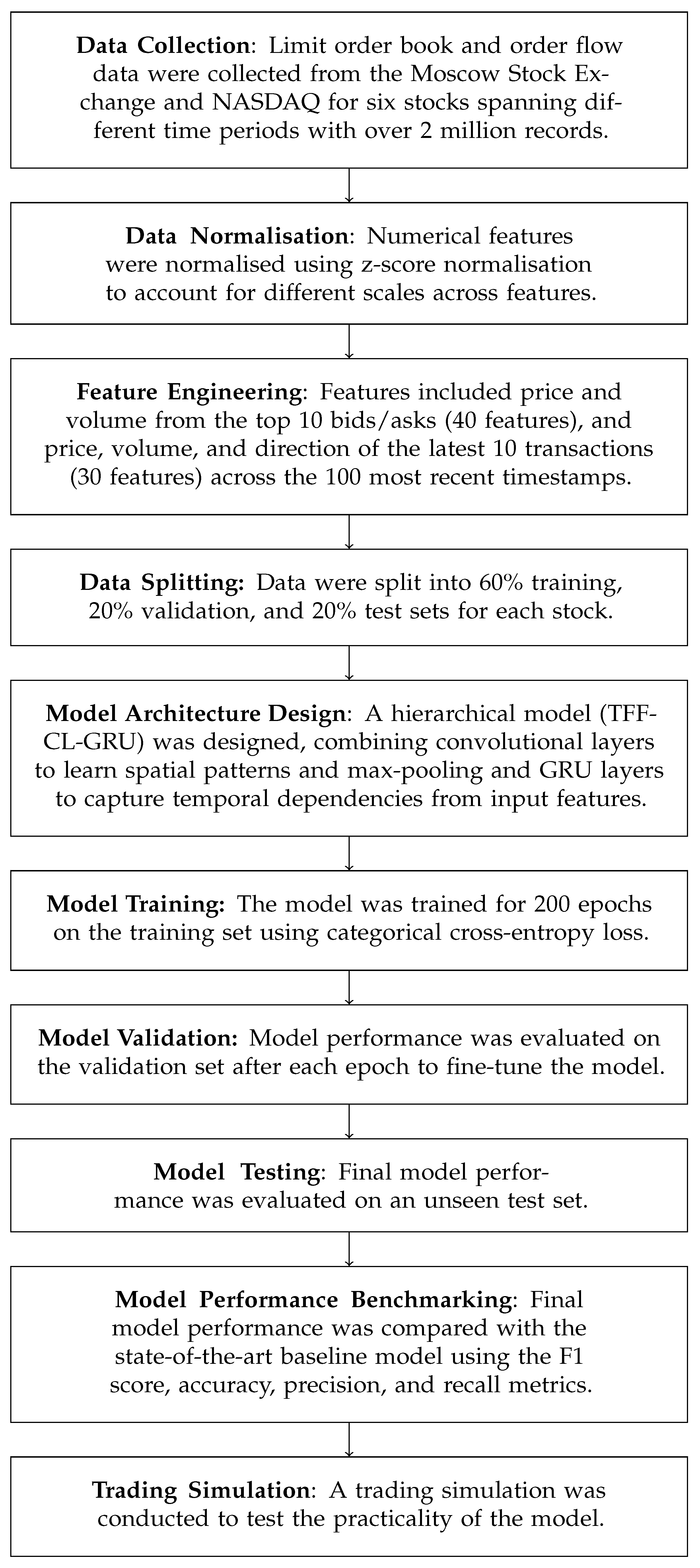
Figure 1 presents a schematic diagram outlining the proposed methodology. The detailed description of the methodology is presented in the following subsections.

4.2. Data Preparation

As mentioned above, the data used in this research experiment are high-frequency stock market data. Before feeding these data to the neural network, we need to perform three main steps:

• Data sourcing;
• Feature selection;
• Normalisation.

Each of the above-mentioned steps is described in detail in the respective subsection below.

4.2.1. Data Sourcing

An open-source benchmark LOB dataset was presented in the work by Ntakaris et al. [27]. It is widely used in the research area and could potentially be leveraged for this work as well. However, it has several limitations:

• It is more than ten years old, which can make it non-representative of the current situation in the dynamically evolving stock market.
• Prices for five stocks are provided, but they are all combined in a single dataset, making the individual stocks indistinguishable.
• It contains only limit order book data but not order flow data.

Due to the aforementioned reasons, it became imperative to generate a dataset that addresses the limitations outlined above. Experimental validation in the study conducted by Doering et al. [15] confirmed that incorporating order flow data alongside limit order book data can enhance the predictive capabilities of a model. Consequently, the decision was made to utilise both types of data as sources for feature extraction. Order flow and limit order book data were collected from the Moscow Stock Exchange through the QUIK workstation for three stocks:

• Sberbank;
• VTB;
• Gazprom.

Considering the focus of this paper on high-frequency intraday trading, even just a few weeks of tick-by-tick data can yield millions of timestamps, ample for training practically any deep learning model in this context. While collecting tick-by-tick data from the market, we set a minimal threshold of 100,000 timestamps for each of the stocks.

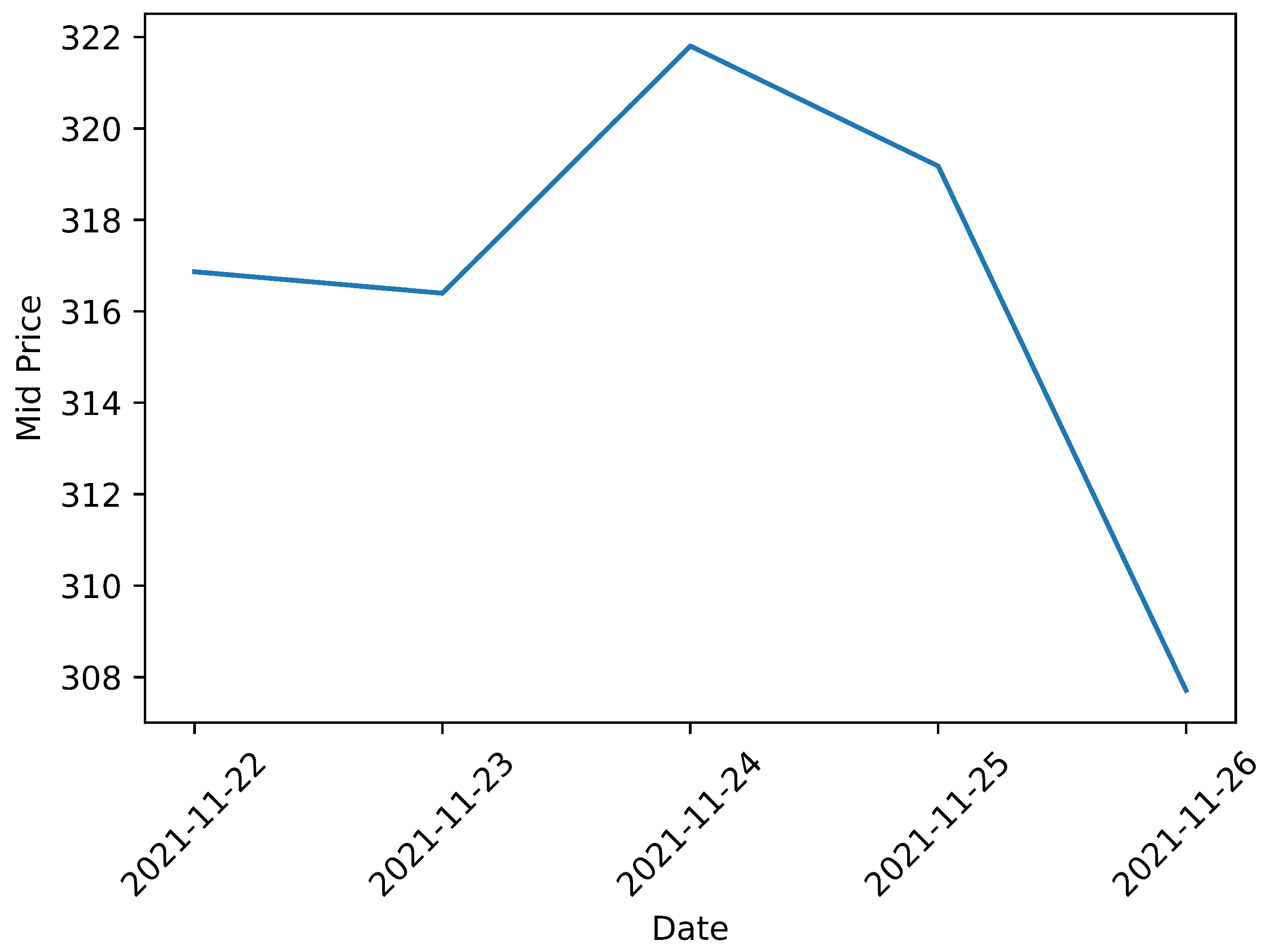
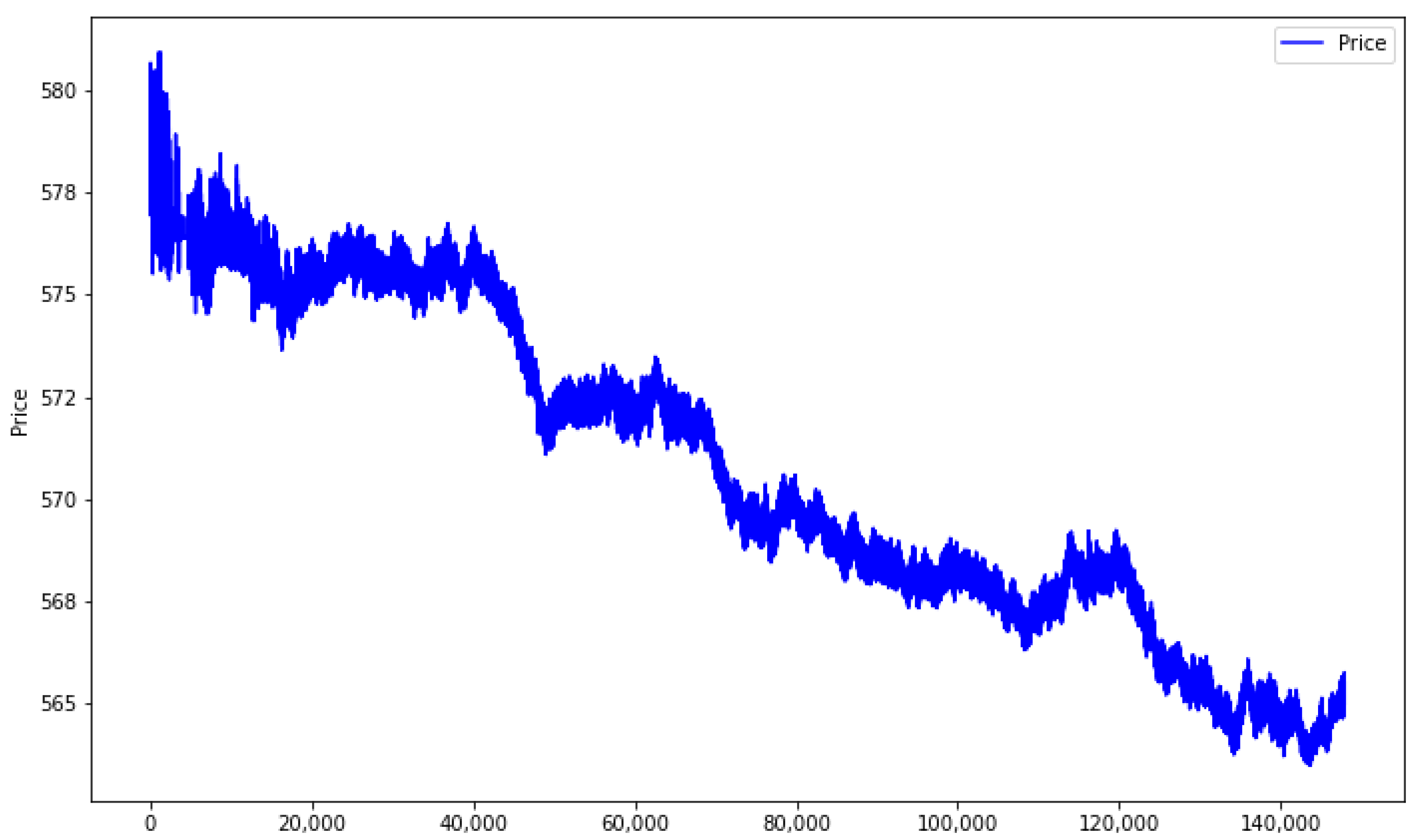
For Sberbank stock, the dataset spans the period from 22 November 2021 to 26 November 2021, encompassing more than 750,000 timestamps in total. The trajectory of the stock during this period is illustrated in Figure 2. Observing the chart reveals that the Sberbank stock experienced growth only on November 23rd; subsequently, it followed a downward trend.

For VTB stock, the dataset encompasses the period from 3 August 2021 to 17 August 2021, comprising more than 550,000 timestamps in total. The trajectory of the stock during this period is illustrated in Figure 3. Examining the chart reveals a robust upward trend, with a corrective phase observed between August 11th and 13th.

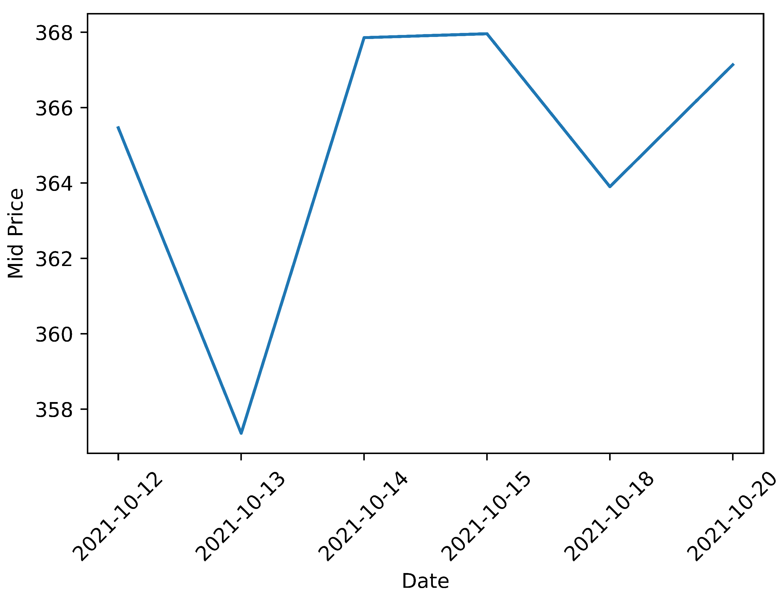
For Gazprom stock, the dataset spans the period from 12 October 2021 to 20 October 2021, encompassing around 410,000 timestamps in total. The trajectory of the stock during this period is illustrated in Figure 4. Observing the chart indicates that after an initial decline, the price returned to almost the same level.

Additionally, to ensure that the model generalises well, we also trained and tested it on three stocks traded at NASDAQ from the existing LOBSTER dataset [36], namely Apple, Amazon, and Google. The data for all three stocks are for 21 June 12.

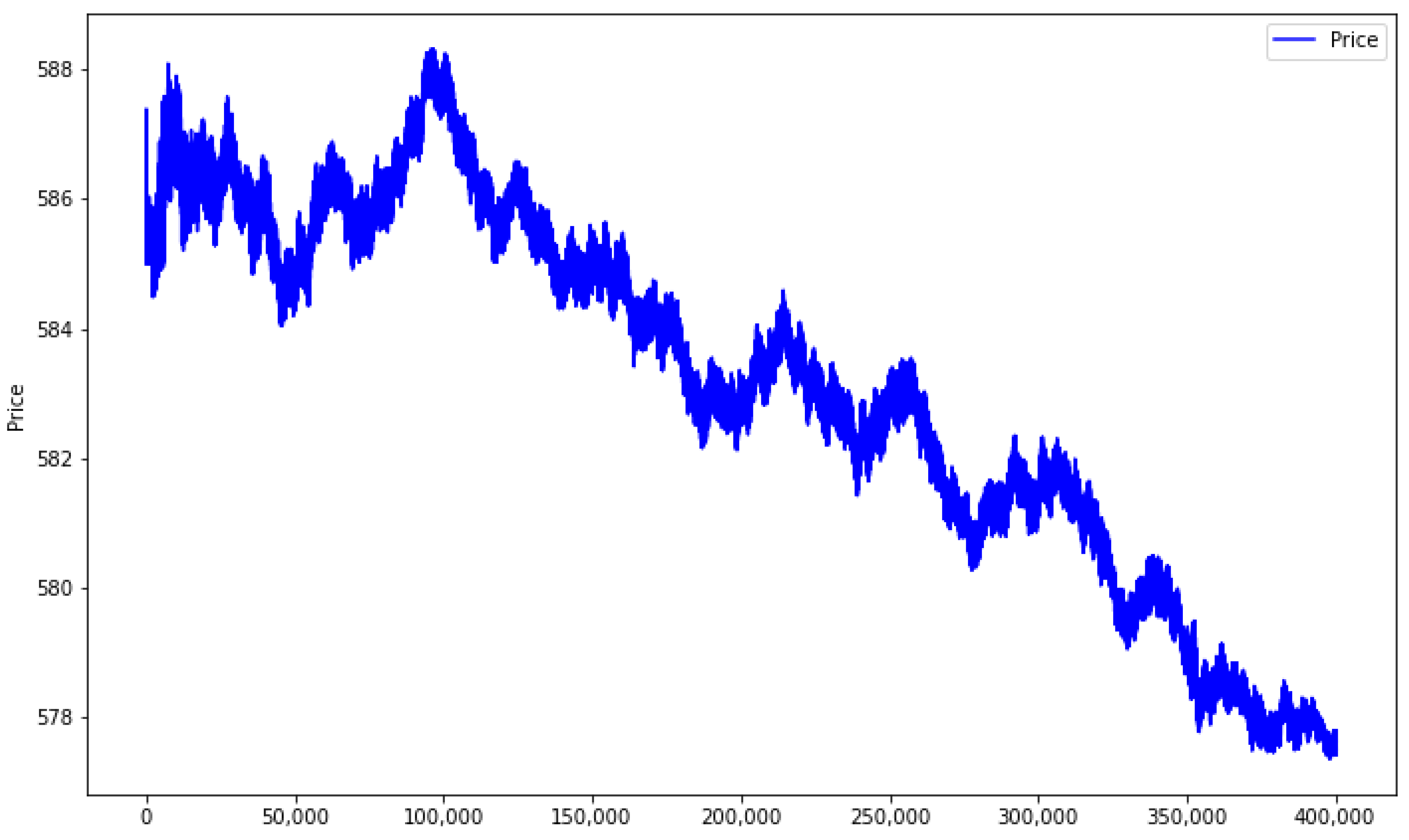
For Apple stock, the dataset encompasses around 400,000 timestamps in total. The trajectory of the stock during this period is illustrated in Figure 5. As can be seen from this chart, the stock was in a downward trend.

For Amazon stock, the dataset encompasses around 270,000 timestamps in total. The trajectory of the stock during this period is illustrated in Figure 6. As can be seen from this chart, the stock was in a downward trend.

For Google stock, the dataset encompasses around 150,000 timestamps in total. The trajectory of the stock during this period is illustrated in Figure 7. As can be seen from this chart, the stock was in a downward trend.

4.2.2. Feature Selection

As elucidated by Gould et al. [37], limit orders at deeper levels are deemed less relevant to price movements. Consequently, it is a common practice to restrict the analysis to the first 10 levels of the limit order book, as demonstrated in the works by Wallbridge et al. [35] and Zhang et al. [10]. This same approach was applied in the current work. We experimented with including additional LOB levels and more transactions but found no significant improvement in model performance. Including too many inputs can overwhelm the model and degrade performance due to increased noise and redundancy in the data.

As confirmed by Doering et al. [15] and through our own experiments, OF data offer additional insights and can enhance the model’s predictive capability by tracking the actual trades executed by market participants. However, to ensure consistency and feasibility in input data tensors for the neural network, it was necessary to limit the number of OF transactions added to the feature space at each timestamp. The alternative, allowing for a variable number of transactions at each timestamp, would result in input data tensors with variable shapes, rendering them incompatible with the neural network. Preliminary analysis revealed that the majority of limit order book timestamps exhibit fewer than 10 OF transactions occurring since the previous timestamp. Consequently, this number was chosen as a practical limit. We acknowledge that further research on this matter could be beneficial.

Thus, at each training iteration, input data are represented by data tensors of shape [100, 70]. In these R100 × R70 tensors, R100 corresponds to the 100 most recent timestamps, R[1-40] pertain to the limit order book features, namely price and volume data for the 10 best bids and the 10 best asks, resulting in 40 features, and R[41-70] represent the order flow features—price, volume, and direction (buy/sell)—for the 10 latest transactions at each limit order book timestamp, contributing 3 × 10 = 30 features.

The LOBSTER dataset has a slightly different representation of the order flow. It has only one order between each consequent LOB timestamp, but in addition to the direction, price, and volume, it also contains event types:

• Submission of a new limit order;
• Cancellation (partial deletion of a limit order);
• Deletion (total deletion of a limit order);
• Execution of a visible limit order;
• Execution of a hidden limit order;
• Cross-trade, e.g., auction trade;
• Trading halt indicator.

For the experiments with the LOBSTER data, input data are represented by tensors of shape [100, 44]. In these R100 × R44 tensors, R100 corresponds to the 100 most recent timestamps, and R[1-40] relate to the limit order book features, namely price and volume data for the 10 best bids and the 10 best asks, resulting in 40 features. The rest, R[41-44], represent the order flow features: price, volume, direction (buy/sell), and event type for the latest transaction at each limit order book timestamp.

The input representation was a key factor in the model’s strong predictive power. By incorporating both LOB and OF data, as well as their temporal characteristics, the model was able to capture diverse patterns from these different but complementary sources of market information. This allowed it to outperform models using only LOB or static input representations. The hierarchical feature-learning architecture was also important for extracting meaningful patterns from this representation.

4.2.3. Normalisation

It is considered best practice to normalise data before feeding them into a neural network. If this is not done, features could have different scales, whereby features with higher values may have excessive weights associated with them during training, while those with smaller values would be neglected. To avoid this and ensure faster learning, normalisation was carried out for the above-described order flow and limit order book data.

Commonly used methods of normalisation were considered to find the one most suitable for the input data used in the experiments:

• Min-max;
• Decimal precision;
• Z-score.

Our empirical findings revealed that the dataset employed in the experiments contained a significant number of outliers—values that were exceptionally high or low. As a result, normalisation methods dependent on maximum or minimum values in their formulas would be notably impacted by these outliers.

To mitigate this, a min-max normalisation method, as its name implies, takes into account both the minimum and maximum values in its calculation. In contrast, the decimal-precision normalisation approach incorporates only the maximum value in the calculation. Simultaneously, the z-score normalisation method relies on the deviation from the average, which is less susceptible to the influence of outliers compared to the two aforementioned approaches.

Thus, normalisation was carried out for the whole dataset using the standard z-score approach, $z=\frac{x_i-\mu }{\sigma }$, where $x_i$ is the value of the feature at the current timestamp, $\mu$ is its mean value, and $\sigma$ is its standard deviation.

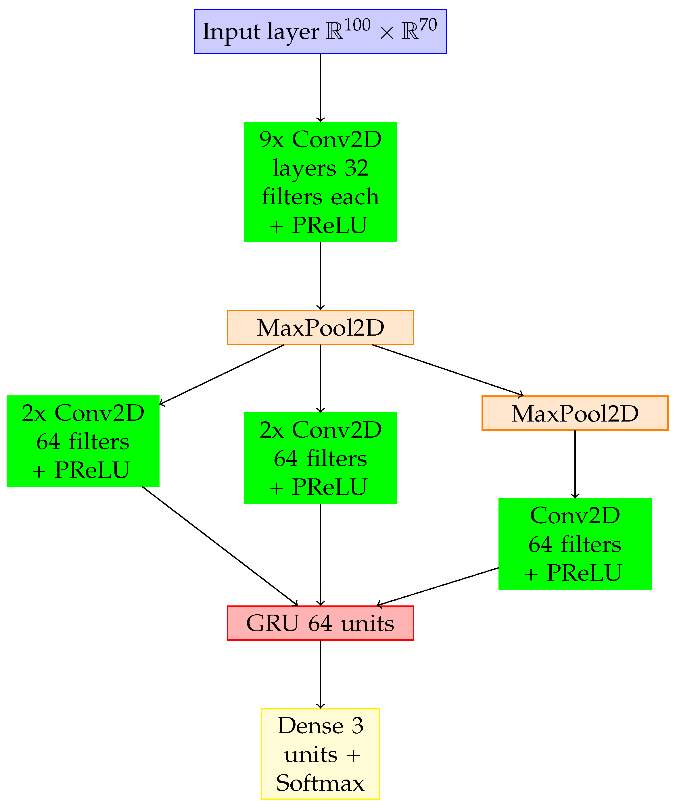
4.3. Model Architecture

As discussed earlier, deep supervised learning models have demonstrated superior performance on the benchmark LOB dataset compared to other methods. As confirmed in the work by Doering et al. [15], convolution layers are very helpful for handling high-dimensional data such as LOB and OF tensors. They serve to automatically extract the most relevant features from these data. To fully account for the time-series nature of the data, recurrent layers are added to the architecture. These layers facilitate the transfer of hidden state information from prior observations to the next ones. These two types of layers, in addition to a standard max-pooling layer applied to make the model less sensitive to small changes in the input data and a dense layer as an output layer, are the key building blocks of the proposed deep neural network architecture. 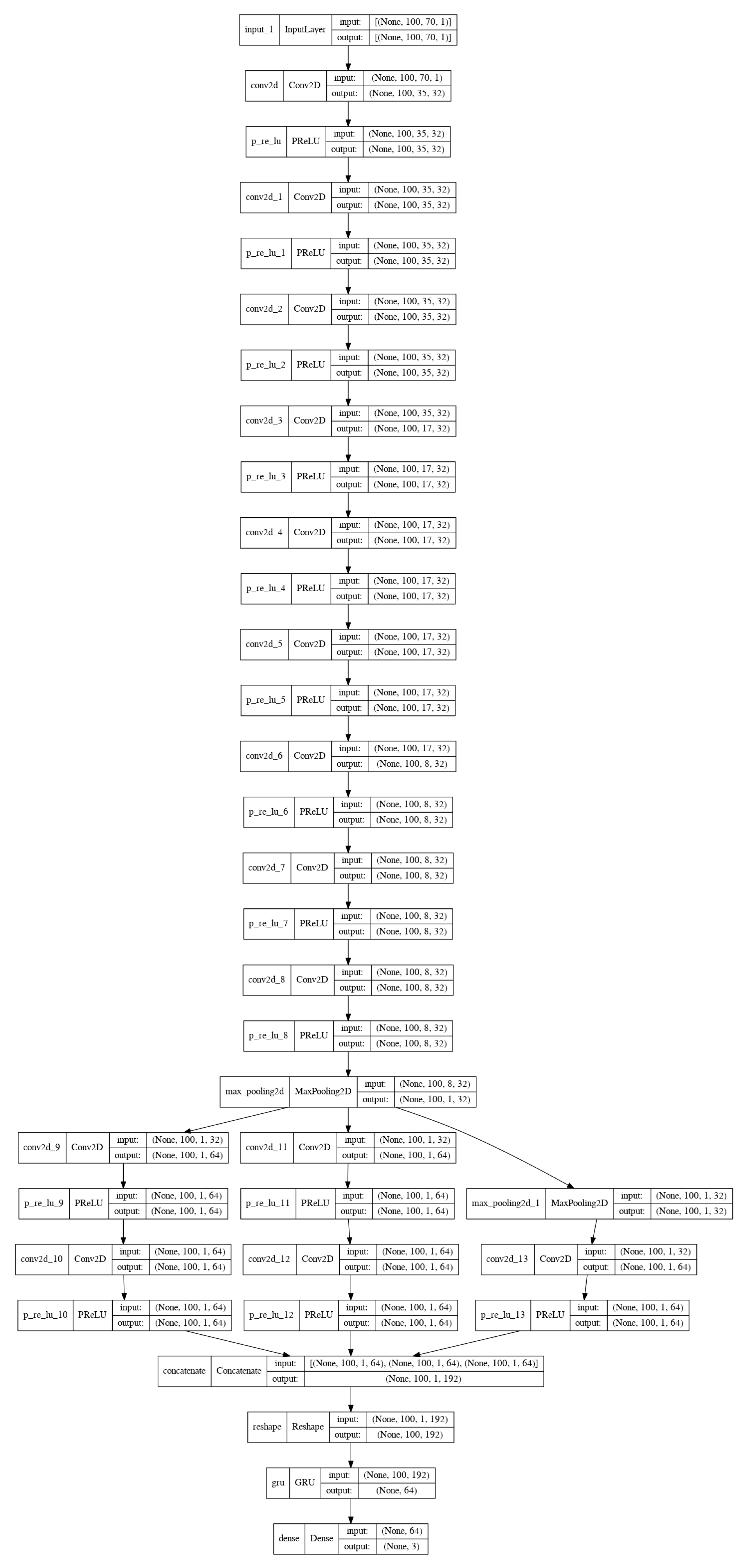In Figure 8, the architecture of the proposed model is depicted at a conceptual level, whereas Figure A1 in Appendix A depicts the detailed architecture.

The input layer receives processed and normalised data in the form of tensors with a shape of [100, 70]. In these R100 $“\times ”$ R70 tensors, R100 corresponds to the 100 most recent timestamps, and R70 relates to the limit order book and order flow features. These input data are transmitted through nine consecutive convolution layers, each with 32 filters, followed by a max-pooling layer (kernel size = 1 × 8; stride = 1 × 1), forming the first block of convolution layers.

The kernel size of the first and sixth layers is 1 × 2; the kernel size of the second, third, fifth, sixth, eighth, and ninth layers is 4 × 1, and the kernel size of the seventh layer is 1 × 10. The second, third, fifth, sixth, eighth, and ninth layers have the same padding. All the layers in the first block have a standard stride of 1 × 1, except for the first and fourth layers, which have a stride of 1 × 2. For all the convolution layers, the parametric rectified linear unit activation function is applied. It was first introduced by He et al. [38] and is a generalisation of the popular rectified unit activation function originally presented by Nair et al. [39]. The parametric rectified linear unit activation function multiplies negative input values $y_i$ by coefficient $a_i$ to obtain outputs $f\left(y_i\right)$, while for positive input values, the output equals the input:

$$\begin{array}{cc}\hfill & y_i>0:f\left(y_i\right)=y_i\hfill \\ \hfill & y_i<0:f\left(y_i\right)=a_i\times y_i\hfill \end{array}$$

The original rectified unit activation function assumes zero output for negative input values, and the output equals the input for positive input values:

$$\begin{array}{cc}\hfill & y_i>0:f\left(y_i\right)=y_i\hfill \\ \hfill & y_i<0:f\left(y_i\right)=0\hfill \end{array}$$

The motivation behind opting for the PReLU lies in its ability to introduce nonlinearity to the network while addressing certain limitations associated with traditional rectified linear unit (ReLU) activations. Unlike the standard ReLU, which can suffer from the “dying ReLU” problem by setting all negative values to zero, the PReLU allows for the adaptation of the negative slope during training. This adaptability contributes to improved convergence during training and better gradient flow, enhancing the model’s ability to learn complex representations from financial data. Additionally, the PReLU has demonstrated effectiveness in mitigating the vanishing gradient problem, which can be especially pertinent in deep neural network architectures. Although the parametric rectified linear unit function adds minor extra computation costs to learn parameter $a_i$, it has been demonstrated that it allows for faster convergence of deep learning models such as TFF-CL-GRU.

The second block consists of three sub-blocks that are concatenated along axis 3. Each of these three sub-blocks receives the outputs from the max-pooling layer of the first block as input. The first sub-block consists of two consecutive convolution layers with 64 filters; stride = 1 × 1; with padding; and with kernel size = 1 × 1 for the first layer and 3 × 1 for the second one. This selection is based on a nuanced understanding of the financial data, where the smaller kernel size (1 × 1) allows for focused, localised feature extraction, capturing fine-grained details critical for discerning subtle patterns in stock price movements. The larger kernel size (3 × 1) in the second layer broadens the scope to capture more extensive contextual information. The second sub-block consists of two subsequent convolution layers with 64 filters; stride = 1 × 1; with padding; and kernel size = 1 × 1 for the first layer and 5 × 1 for the second one. This choice is grounded in the need for the model to adapt to diverse scales of features present in financial data. The smaller kernel size (1 × 1) again prioritises localised details, whereas the larger kernel size (5 × 1) extends the receptive field to incorporate global context, allowing the model to grasp larger-scale patterns in stock price movements. The third sub-block consists of a subsequent max-pooling layer with kernel size = 3 × 1; stride = 1 × 1; and with padding, and a convolution layer with 64 filters; stride = 1 × 1; with padding; and with kernel size = 1 × 1. The inclusion of the max-pooling layer serves to downsample the data, reducing dimensionality while retaining essential features. The subsequent convolution layer with a smaller kernel size (1 × 1) focuses on further refining the extracted features. The rationale behind these choices lies in optimising the network’s ability to discern patterns at different scales, facilitating hierarchical feature learning tailored to the unique characteristics of financial data. The parametric rectified linear unit (PReLU) activation function is also applied for all the convolution layers in the second block as was done for the first block. The overarching architectural decisions, including the specific kernel sizes, number of filters, and strides, are informed by a data-driven approach and empirical studies, ensuring that the model is adept at extracting meaningful features for precise and accurate stock price predictions.

The resulting 3D tensor is reshaped to 2D to match the input shape of the consequent Gated Recurrent Unit (GRU) layer with 64 units. The decision to incorporate a GRU layer is rooted in the need for the model to effectively capture temporal dependencies and hierarchical representations in the sequential financial data. This is particularly crucial in the context of stock price movements, where the historical sequence of prices holds valuable insights into potential future trends. The GRU’s gating mechanism allows it to selectively update and memorise information, mitigating the vanishing gradient problem and facilitating the learning of long-term dependencies.

The GRU layer, in turn, is connected to the final dense layer with three neurons, each of them corresponding to one of three output classes (“upward”, “flat”, “downward”). For this final layer, the softmax activation function [40] is used to distribute the outcome probability among these three classes. The output from this function $f{\left(x\right)}_i$ for the i-th element ($x_i$) of input vector x, consisting of K elements, is defined according to the formula $f{\left(x\right)}_i=\frac{e^{x_i}}{{\sum }_{j=1}^K{e}^{x_j}}$, where K is the number of classes (three in this case).

The configuration of the TFF-CL-GRU model, including the determination of the number of layers, units, filters, kernel sizes, strides, padding, and other characteristics, was systematically chosen to optimise its overall performance. This process involved iteratively fine-tuning these architectural parameters to enhance the model’s capacity to learn intricate patterns and relationships from the training data.

4.4. Experimental Design

The TFF-CL-GRU model is trained separately for each of the three stocks from our dataset (Sberbank, VTB, Gazprom) for 200 epochs. The first 60% of the dataset is used for training, the next 20% is used for validation, and the remaining 20% is used for testing. The purpose of the validation set is to find the optimal neural network configuration and fine-tune its parameters while still keeping the test set out of this sample, thus minimising the risk of overfitting.

The performance of the TFF-CL-GRU model is evaluated against other state-of-the-art models based on standard statistical measures such as accuracy, precision, recall, and F1 score. These four metrics are defined as follows:

$$Accuracy=\frac{TP+TN}{TP+TN+FP+FN}$$

$$Precision=\frac{TP}{TP+FP}$$

$$Recall=\frac{TP}{TP+FN}$$

$$F1score=2\times \frac{Precision\times Recall}{Precision+Recall},$$

where TP represents true positive; TN represents true negative; FP represents false positive; and FN represents false negative in relation to the comparison of the stock prediction with the actual price. From these metrics, the fairest picture for this experiment is provided by the F1 score. Importantly, in this case, accuracy is misleading as the dataset is not balanced among the three labels. The F1 score is the harmonic mean of precision and recall and thus can handle unbalanced classes by finding the optimal balance between type I and type II errors.

As outlined in Section 2, the state-of-the-art DeepLOB model [10] is selected as a benchmark to gauge the performance of the TFF-CL-GRU model.

Another crucial consideration for stock price prediction is its practicality. Executing a trading strategy in real market conditions is a complex task, involving numerous considerations. Even the ability to correctly predict the direction of a price change does not guarantee the profitability of the trading strategy. For instance, if the magnitude of the price increase or decrease is lower than the bid–ask spread, executing a round transaction with market orders may lead to losses, even if the price moves as anticipated. Additionally, short sales may not always be available to investors, and even if they are, additional commissions might outweigh the potential gains from short-selling falling stocks. Liquidity is another significant factor, where a limited number of stocks on the ask or the bid side can hinder investors from buying or selling the required amount of stock. These are just a few of the factors that must be considered in a real-world trading strategy.

To account for these factors, a decision was made to devise a simple trading strategy based on the predictions of our model and conduct trading simulations using actual market data. This strategy executes market buy/sell orders whenever the model outputs the buy/sell signal, with a confidence level of at least 90%. Short sales are prohibited, and trading commissions are assumed to be zero, considering that many brokers offer this. However, the bid–ask spread is considered a trading cost. The amount of each transaction is limited by the best bid/ask volume. The starting balance is set to 1000 times the share price, aiming to minimise the market impact of these transactions.

Additionally, a “buy-and-hold” strategy is introduced to provide a basis for comparative performance assessment. Following this strategy, stocks are acquired at the beginning of each simulation at the best ask price, purchasing the available volume at that price in each iteration until the full initial balance is invested in stocks. These stocks are then held until the end of the simulation.

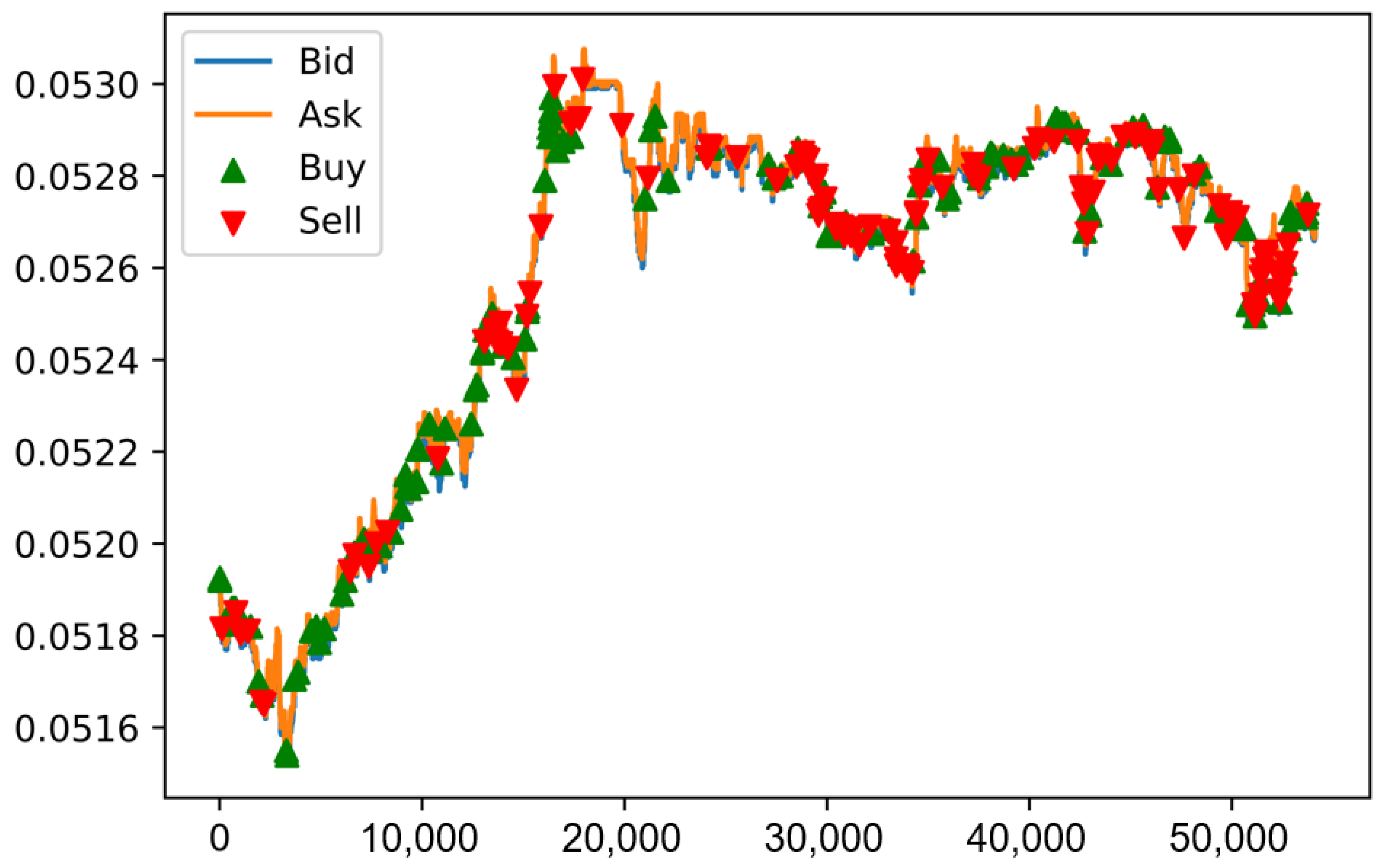
One thousand trading simulations are conducted for each of the three stocks: VTB, Sberbank, and Gazprom. Each trading simulation contains a randomly ordered sample of limit order book (LOB) prices and volumes, with the number of events equivalent to one trading day. To illustrate the process, one trading simulation for VTB stock is presented in Figure 9.

In order to measure the strategy performance, the returns on investment for each trading simulation are calculated as follows:

$$Returnoninvestment=\frac{Endingbalance+(Numberofstocksacquired \times Endingbidprice)}{Startingbalance}-1$$

To make the results easier to interpret, these daily returns are converted to annual returns, as follows:

$$AnnualReturn={(1+\left(Returnoninvestment\right))}^{260})-1),$$

where 260 is the number of working days in a year.

5. Experimental Results

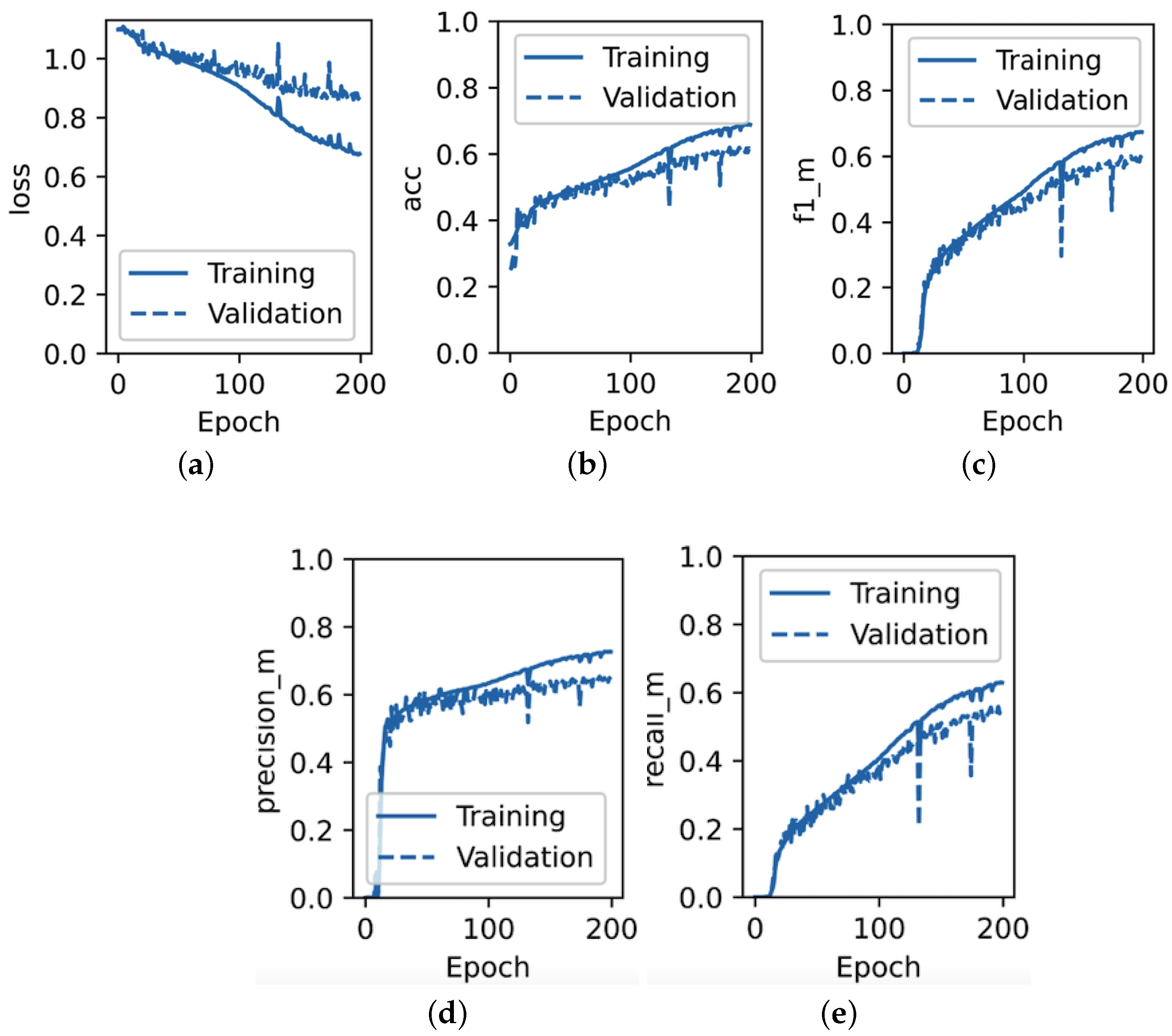
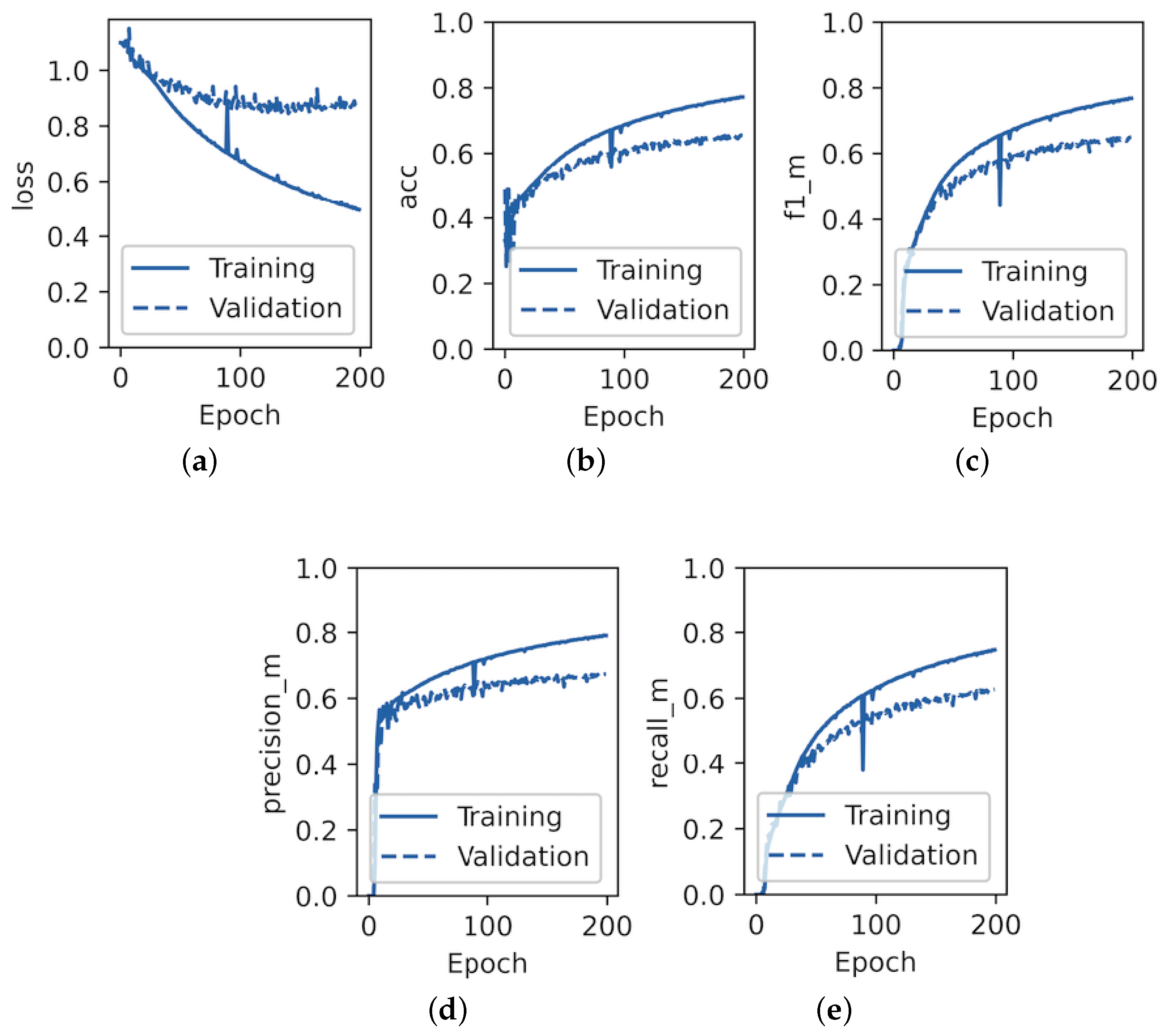
In accordance with the experimental design outlined above, the training and validation performance for VTB stock from the MICEX dataset for both the state-of-the-art DeepLOB model and the proposed TFF-CL-GRU model is presented in Figure 10 and Figure 11, respectively.

As observed in Figure 10 and Figure 11, by epoch 200, the F1 score for the validation set of the state-of-the-art DeepLOB model barely reached 60%, whereas for the TFF-CL-GRU model, it clearly exceeded it by at least 5pp. The F1 score curves for both the validation and training datasets did not reach a plateau by epoch 200, indicating the potential for further improvement with an extended experiment. However, considering that the training curve started to deviate substantially from the validation curve, signalling an increasing risk of overfitting, and to maintain the experiment’s time-bounded nature for comparability with other researchers in this field, the decision was made to conclude the experiment at this point.

In terms of accuracy, precision, and recall metrics, the TFF-CL-GRU model also outperformed the DeepLOB model. The experiment was repeated for six stocks, and it can be seen in

Table 4. Performance comparison of the TFF-CL-GRU model and the DeepLOB model for six stocks.

Model	Metric	VTB	Sberbank	Gazprom	Apple	Amazon	Google
TFF-CL-GRU	Accuracy	66%	48%	53%	50%	60%	55%
	F1 score	65%	45%	51%	49%	60%	55%
	Precision	67%	51%	56%	51%	61%	55%
	Recall	63%	40%	47%	47%	59%	54%
DeepLOB	Accuracy	62%	49%	52%	41%	40%	42%
	F1 score	60%	41%	46%	31%	36%	38%
	Precision	66%	54%	57%	42%	40%	42%
	Recall	55%	34%	39%	25%	32%	34%

that the TFF-CL-GRU model consistently outperformed the state-of-the-art DeepLOB model in terms of the F1 score for each of them.

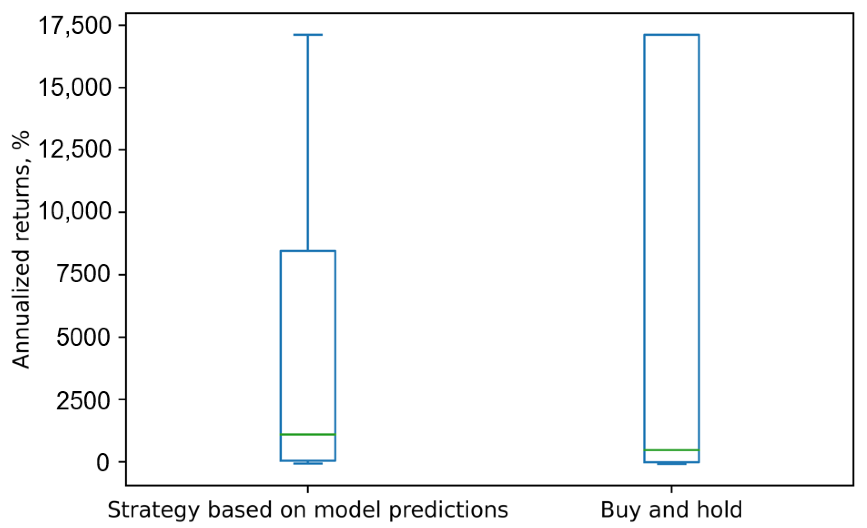
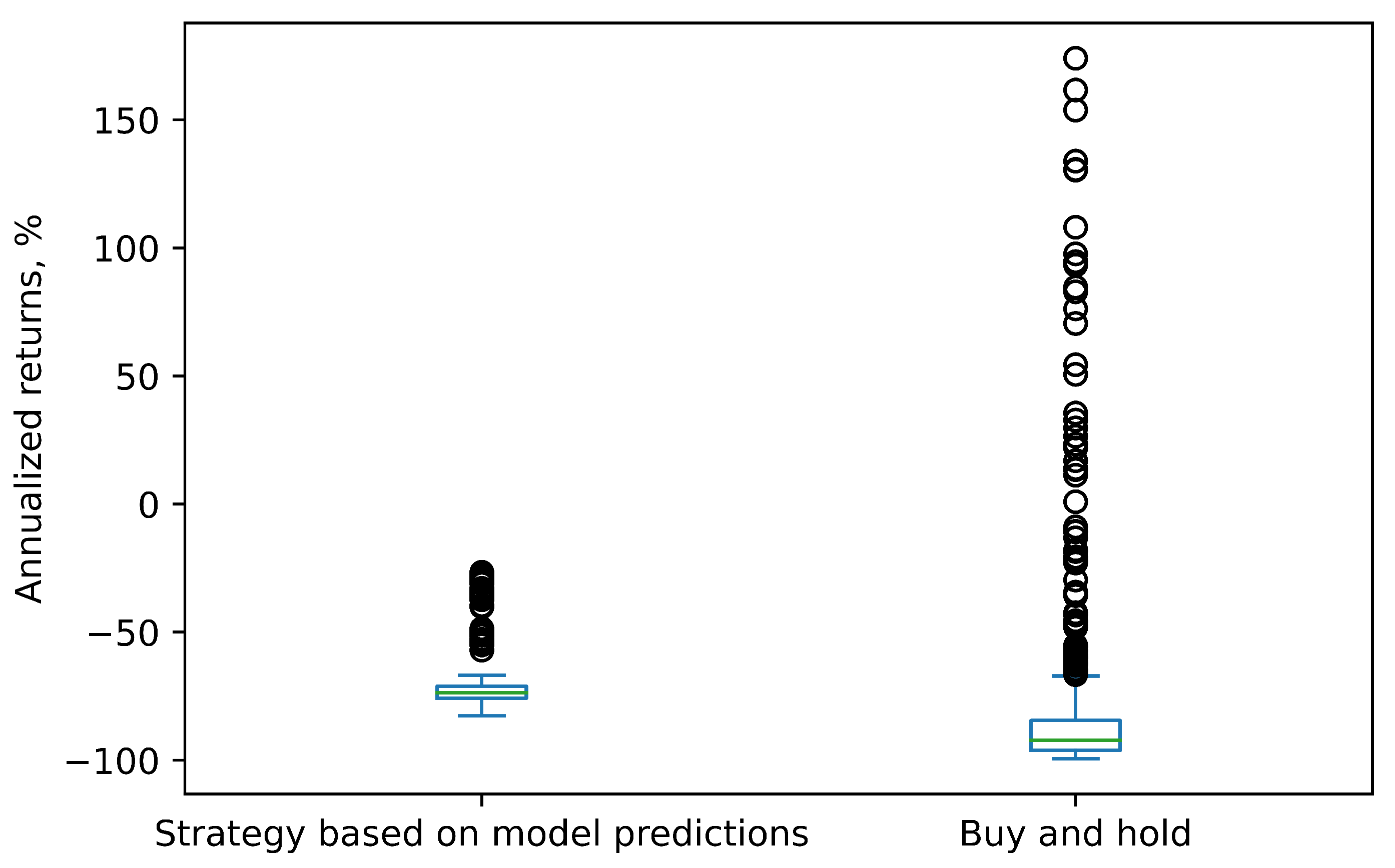
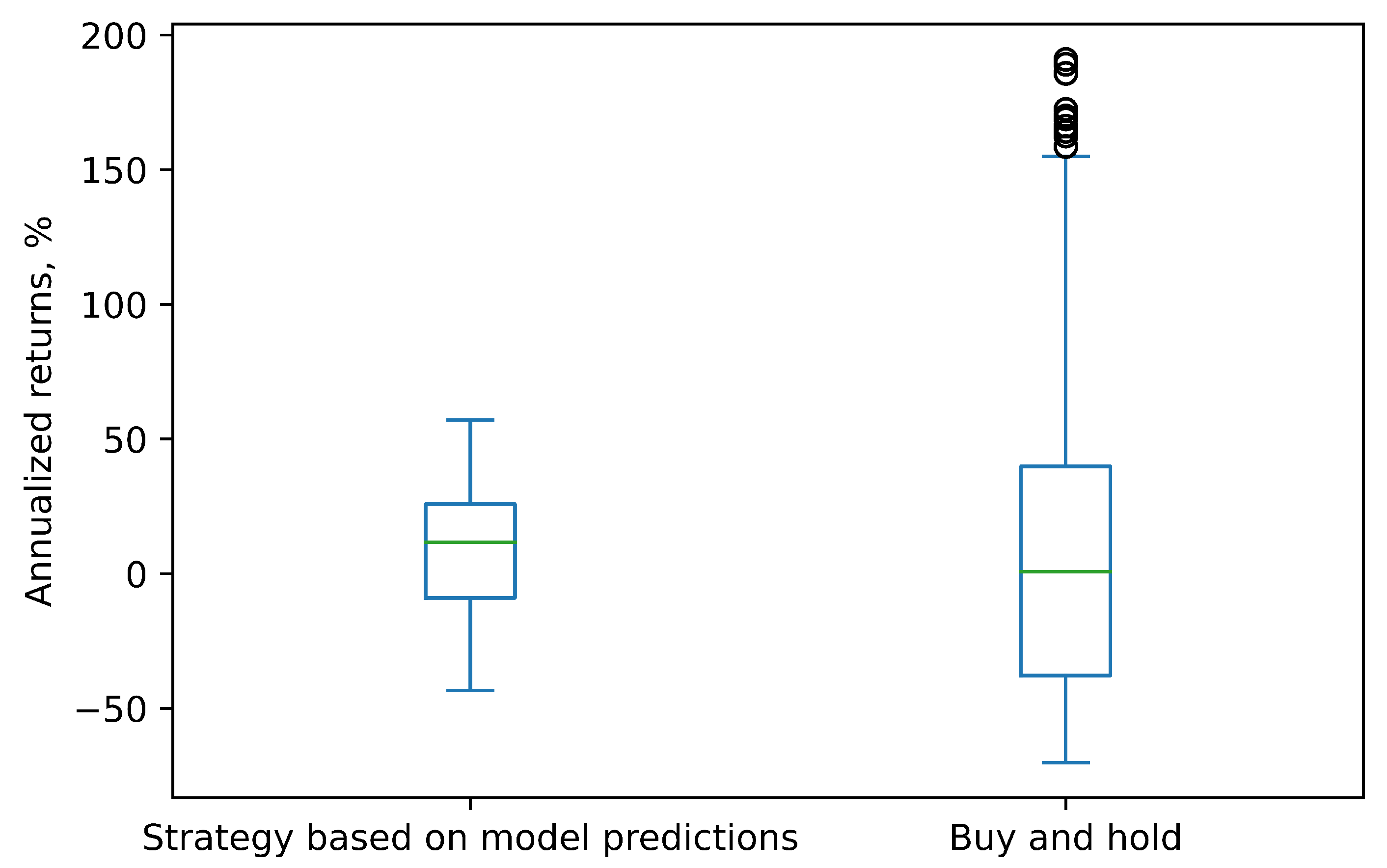
The practicality of the TFF-CL-GRU model was also evaluated through trading simulations. The annual returns for the strategy based on our model’s predictions and the buy-and-hold strategy for each of the three stocks (VTB, Sberbank, and Gazprom) are presented in Figure 12, Figure 13 and Figure 14, respectively.

As depicted in these charts, for all three stocks, the strategy based on our model’s predictions generated median returns that were higher than those of the buy-and-hold strategy and in the positive zone, except for Sberbank. The negative returns for Sberbank stock can be explained by the fact that this stock was predominantly in a declining trend, and short sales were prohibited. For the same reason, it would not make sense to create trading simulations for Apple, Amazon, and Google stocks, considering they were all in a downward trend.

However, the VTB stock exhibited a very strong growth trend, with some days experiencing price increases exceeding 2%, resulting in abnormally high annual returns. This consistent growth trend likely simplified the task of predicting the direction and contributed to better model performance in terms of F1 score, accuracy, precision, and recall for this stock compared to the other two. It is important to note that stocks tend to exhibit mean reversion, and a period of rapid growth will likely be followed by a significant decline, leading to more modest annual returns in practice.

Another observation is that the outcomes of the buy-and-hold strategy were much more volatile. The real-world stock market factors previously discussed, such as the bid–ask spread, liquidity limitations, etc., could have also negatively impacted the strategy returns in the simulations.

6. Conclusions and Future Work

The primary objective of this research study was to construct a stock price prediction model utilising deep supervised learning with high-frequency limit order book (LOB) and order flow (OF) market data. Expanding upon previous investigations in this domain, a novel deep supervised model, namely the TFF-CL-GRU model, was developed. This model combines the strengths of convolutional layers to handle the high-dimensional LOB and OF features and recurrent GRU layers to accommodate the time-series nature of the data.

The collected high-frequency market data, including order flow and limit order book data, underwent several steps of data processing, including data sourcing, feature selection, and normalisation. Feature selection involved considering the 100 most recent events in the order flow and limit order book data to capture the time-series nature of the stock price movement. Limiting the analysis to the first 10 levels of the limit order book and setting a limit on the number of transactions at each timestamp ensured consistency in the input data tensors.

Datasets for Sberbank, VTB, Gazprom, Apple, Amazon, and Google stocks were used in the experiment. Based on the analysis of the capabilities of state-of-the-art models in this field, the DeepLOB model [10] was selected as the benchmark for comparative assessment. This decision was influenced by its performance on the benchmark LOB dataset, as demonstrated by Ntakaris et al. [27], and the availability of the code to reproduce the experiment.

The TFF-CL-GRU model demonstrated markedly better performance in terms of its F1 score, which was at least 4% higher than that of the DeepLOB model for each of the six stocks considered. This advantage can be attributed to a combination of feature engineering, model architecture, and the fine-tuning of its parameters. The F1 score achieved by the TFF-CL-GRU model was 45% for Sberbank stock; 51% for Gazprom stock; 65% for VTB stock; 49% for Apple stock; 60% for Amazon stock; and 55% for Google stock. This is much higher than random prediction (which would have been around 33% for three classes) and, in theory, should provide a noticeable advantage in trading. In order to confirm if this was indeed the case, further trading simulations were conducted. The annual returns for the strategy based on the TFF-CL-GRU model’s predictions were measured for each of the three stocks (VTB, Sberbank, and Gazprom). While the strategy relying on the model’s predictions consistently yielded higher median returns for VTB and Gazprom compared to the buy-and-hold strategy, the results differed for Sberbank. The negative returns for Sberbank can be attributed to its predominantly declining trend, compounded by restrictions on short sales.

While the proposed TFF-CL-GRU model demonstrated strong predictive performance on the test datasets, its complexity and computational demands need to be addressed to enable practical deployment in real-time trading environments. Future work should explore techniques for optimising model efficiency without significantly compromising accuracy. Possibilities include pruning redundant connections, quantizing weights, developing lightweight variants of the CNN and GRU blocks, and applying techniques like knowledge distillation, model compression, and multi-task learning to learn a more efficient model from the existing one.

To enhance the ability of the model to generate profits in real stock market conditions, it is crucial to optimise it for various other factors, such as bid–ask spread, stock liquidity, capital limits, etc. However, incorporating these factors within the supervised learning paradigm poses challenges since the optimal execution strategy, considering specific market situations and factors, is not observable. To tackle this complex task, reinforcement learning offers a potential solution. Embedding the existing supervised model within a more sophisticated reinforcement learning framework can address the limitations and enable the consideration of additional factors.

It is important to note that the current supervised model remains valuable as it effectively predicts the stock price direction, which is a critical aspect of trading. By integrating the supervised model with a reinforcement learning framework, it becomes possible to account for a wider range of factors and improve the performance of the model in real-world trading scenarios.

Overall, future work should focus on addressing the limitations identified in the current study, refining the model’s performance, and exploring new avenues to enhance its effectiveness and practical applicability in real-world trading scenarios. One approach to achieve these goals is by leveraging the reinforcement learning framework.