Sensorimotor Control Using Adaptive Neuro-Fuzzy Inference for Human-Like Arm Movement

Abstract

In this study, a sensorimotor controller is designed to characterize the required muscle force to enable a robotics system to perform a human-like circular movement. When the appropriate muscle internal forces are chosen, the arm end-point tracks the desired path via joint-space feedback. An objective function of the least-change rate of muscle forces is determined to find suitable feedback gains. The parameter defining the muscle force is then treated as a learning parameter through an adaptive neuro-fuzzy inference system, incorporating the rate of change of muscle forces. In experimental section, the arm motion of healthy subjects is captured using the inertial measurement unit sensors, and then the image of the drawn path is processed. The inertial measurement unit sensors detect each segment motion’s orientation using quaternions, and the image is employed to identify the exact end-point position. Experimental data on arm movement are then utilized in the control parameter computation. The proposed brain–motor control mechanism enhances motion performance, resulting in a more human-like movement.

1. Introduction

In recent decades, there has been significant interest in developing robotic systems capable of mimicking human movements [1]. The main motivation behind designing such systems is to enhance the versatility and adaptability of robotic systems in various environments, especially those involving human engagement [2]. Applications involving the mimicking of human movements are numerous and range from from human–robot collaboration [3] to rehabilitation [4]. Research on human activities, such as object manipulation [5] and walking [6], requires collaboration across various fields, including kinesiology, physiology, and robotics [7]. Despite advancements in these fields, ongoing research continues to explore the mechanisms that enable human beings to execute such sophisticated movements smoothly.

The human body is supervised by the central nervous system (CNS), comprising the brain, the spinal cord, and the nerves [8]. Single nerve cells in the spinal cord establish connections and convey messages between the brain and the human body [9]. Any spinal cord injury-induced damage results in changes in strength, sensation, and other human body functions below the injury site. The injured spinal cord is unable to transmit and receive messages between the brain and the human body [10]. Individuals with spinal cord injuries can benefit from robotic exoskeleton systems to assist with mobility and movement [11]. Such systems stabilize the patient’s hands, arms, torso, core, legs, and feet, assisting individuals with motion disabilities in regaining motor function through rehabilitation training [12].

In rehabilitation, integrating human-like movements is essential to empower patients in recovering their ability to perform daily activities, ensuring the rehabilitation process is practical, functional, and personalized to each individual’s unique needs [13]. The importance of incorporating these natural movements is particularly apparent in using rehabilitation robots. Accordingly, the control mechanisms for these robots require knowledge of natural human activity. However, while applications of human movements have been explored, performing human-like actions remains considerably challenging [14]. A significant factor contributing to the challenge is the complexity of ill-posed problems arising from the inherent joint and muscle redundancies. Moreover, the coupling between the muscle and joint spaces in the human body presents an additional obstacle. The nonlinear properties of muscles also add another complexity to the control of human-like actions [15]. In order to handle such challenges and perform human-like movements, model-free and model-based control approaches have been developed for the musculoskeletal systems.

Several model-free control designs are addressed in the literature [16,17,18,19]. To generate the muscle activation, deep neural networks (DNNs) are trained with inverse dynamics and optimal control for the point-to-point reaching movements [16]. A biomimetic sensorimotor structure is developed in [17] to control a human musculoskeletal model. Based on visual information, the authors partition the human body into separate modules that regulate muscle activations for specific body regions. Then, they generalize the method to encompass a comprehensive human biomechanical simulation with a sensorimotor control system comprising connected DNNs. In addition to the supervised learning techniques discussed in [16,17], there have been efforts to apply reinforcement learning algorithms for the reaching movements, as studied in [18,19]. In the study by Huang et al. [18], a learning rule employing a recurrent neural network (RNN) is introduced for high-level motor control in a musculoskeletal robot. Meanwhile, Chen et al. [19] proposes a motion learning framework inspired by human movements for a musculoskeletal system, which involves identifying muscle synergies and implementing an iterative learning controller. However, while model-free controllers offer benefits such as simplicity and adaptability, their lack of a precise model can lead to challenges in predicting system behavior, requiring extensive data for training and potentially resulting in less precise control in complex musculoskeletal systems.

In model-based control methods, computing muscle force mostly relies on inverse kinematics, inverse dynamics, and muscle-force optimization approaches. Various model-based control designs have been examined to find the required muscle force, allowing the robotics systems to perform human-like movements. Arimoto et al. [20] demonstrate that a redundant planar robot can achieve human-like multi-joint reaching movement. They employ a feedback approach from task space to joint space to accomplish a motion task, incorporating linear joint angular velocity feedback without solving inverse kinematics. Tahara et al. [21] design a task-space feedback controller including the nonlinear muscle model characteristics for the reaching movements. The desired trajectory is formulated within the task space, and the controller is designed using muscle-space parameters, such as muscle length and contractile velocity. These muscle-space variables are obtained by performing inverse kinematics, transitioning from the task space to the muscle space. Since the motion of the musculoskeletal system can be represented in various spaces, including muscle space, joint space, and task space, the effectiveness of the controller is impacted by the choice of the space in which the controller is designed.

In order to improve the control design performance of the approach suggested in [21], as well as its robustness against possible noise sources, an iterative learning control algorithm using plural space variables is introduced in [22]. Two studies [23,24] introduce adaptive robust control designs for the humanoid robot arms with biarticular muscles to handle the effects of the uncertain dynamic parameters and disturbances. The adaptive algorithms introduced in [23,24] update the dynamics parameters online and handle the dynamic parameter perturbation and disturbance during the movement. An adaptive optimal multi-critic based controller is designed in [25] for a multi-input multi-output musculoskeletal arm model. The fundamental concept behind the design of the adaptive optimal control is to possess the ability to adapt to dynamic parameter changes while determining the muscle force optimized in real-time. Because of the real-time responsiveness and robustness against the uncertainties in sliding mode control architectures, Zhao et al. [26] employ a trajectory tracking control utilizing a switched sliding mode controller in a manipulator powered by pneumatic artificial muscles and Xiuxiang et al. [27] introduces an adaptive fuzzy sliding mode control approach to track the elbow joint and endpoint of the human arm. It is important to remark that most existing model-based controllers have used a simplified version of the musculoskeletal system and such model simplification might not replicate the full range of human movements with high fidelity. For details on musculoskeletal control, the reader is referred to [28].

The main objective of this paper is to outline an effective control strategy that mimics human movement. This paper proves that the developed controller identifies the necessary muscle activation that minimizes the force discrepancy between muscle and arm movement models about the null-space vector. A Hill-type muscle model is employed in a three-link musculoskeletal model with nine muscles in a curved arrangement, including six monoarticular muscles that cross multiple/two joints and three biarticular muscles responsible for shoulder, elbow, and wrist joint movement. The calculation of muscle activation has two components: the model-based joint space controller term and the null-space term, determined via a model-free learning algorithm. The null-space term plays a significant role in rendering the movement more human-like, and it is typically considered as a constant rather than being calculated from real-time motion data. The approach in this study to ascertain the suitable null-space term involves reducing the force difference between the muscle and arm movement models using the Adaptive Neuro-Fuzzy Inference System (ANFIS). An assemblage of exemplars with a three-link arm has been incorporated to illustrate the application of the developed control algorithm. The simulation results have also been included to corroborate the performance quality of the proposed control methodology.

The rest of this work is organized as follows. Section 2 introduces a kinematic and dynamic model of the musculoskeletal arm model. Section 3 presents the sensorimotor control architecture for human-like arm movement. Section 4 introduces the experimental design, materials, and methods. Section 5 summarizes the main results. Section 6 concludes the article.

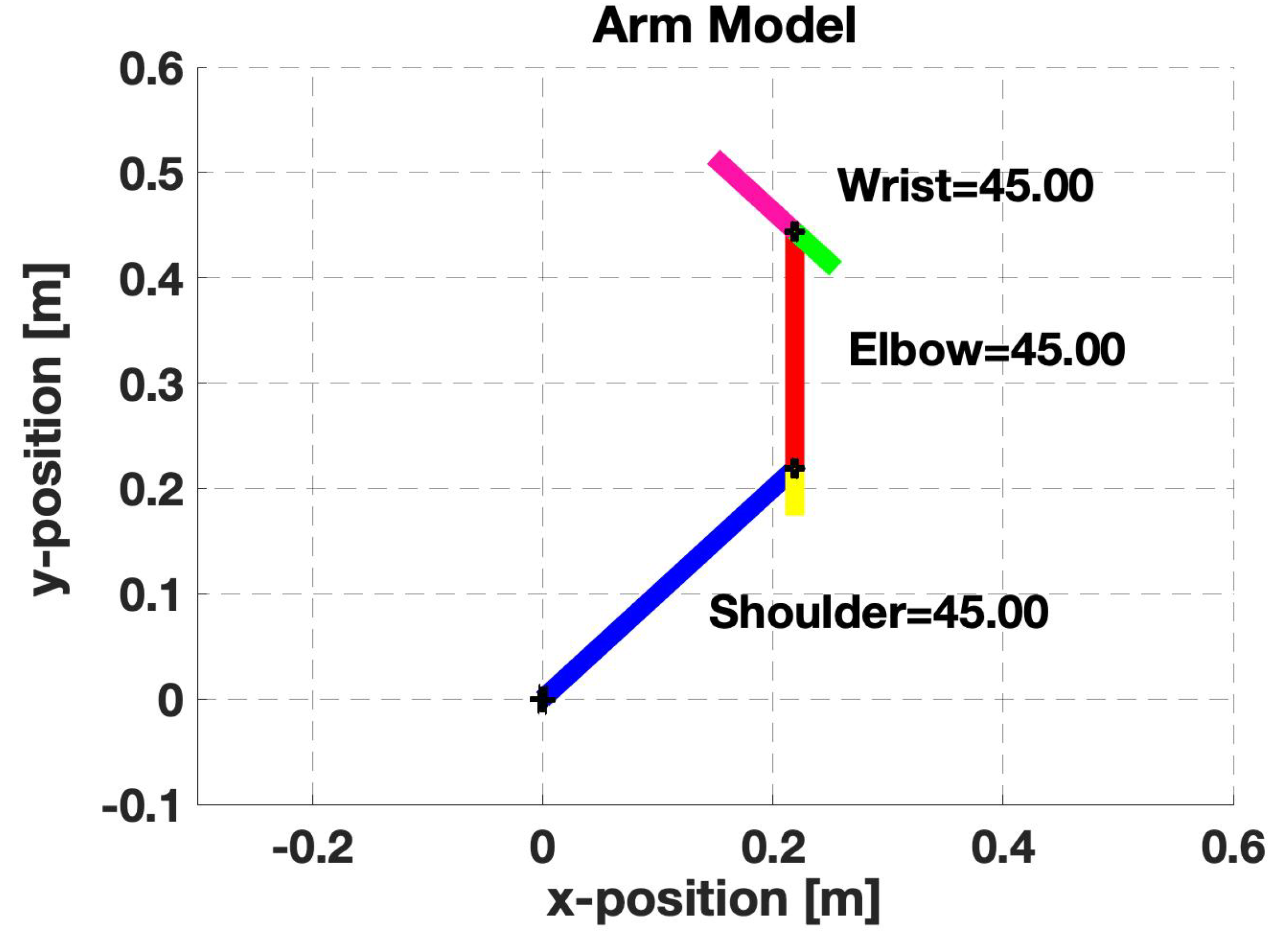
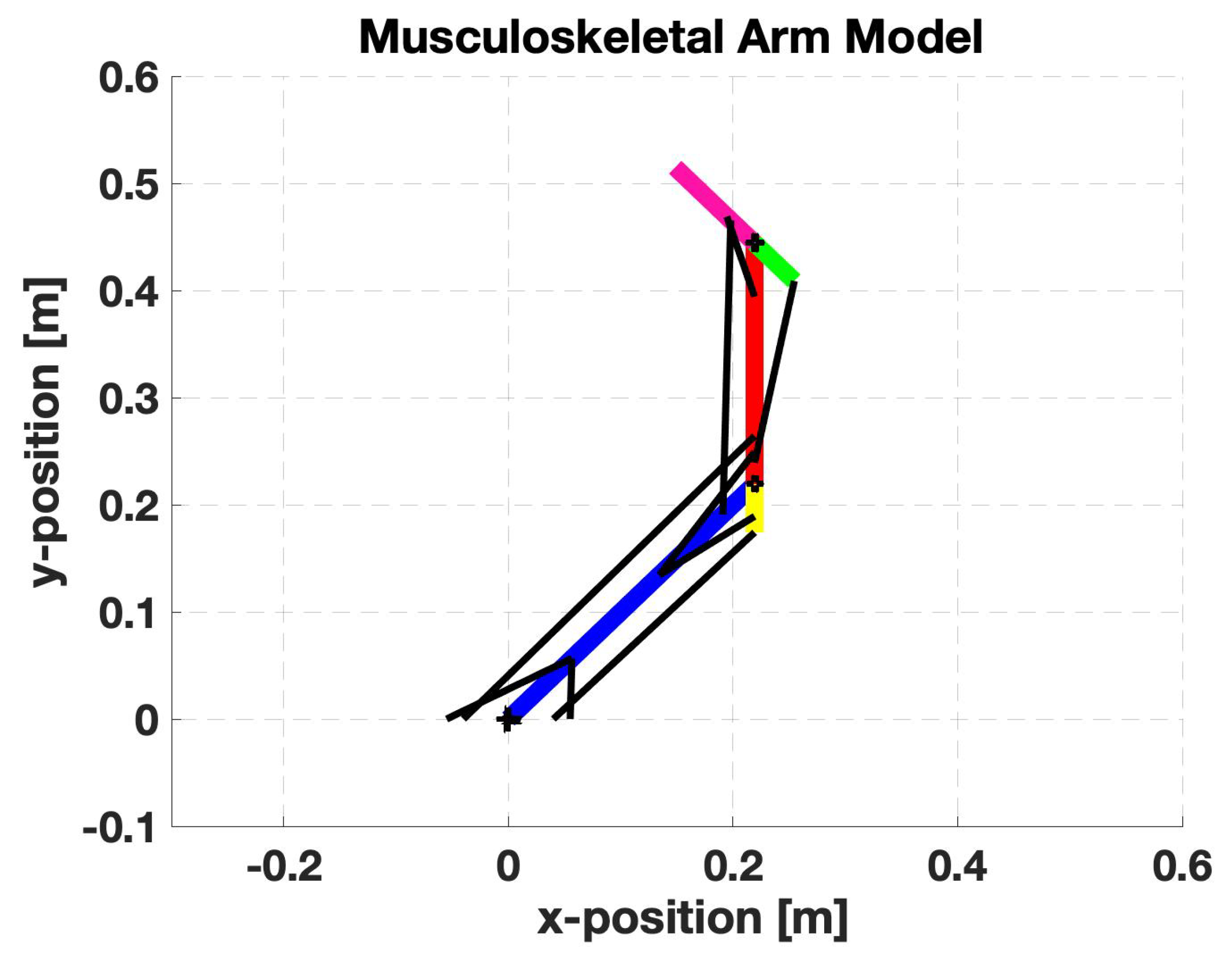
2. Musculoskeletal Modeling

This section introduces a musculoskeletal arm’s kinematic and dynamic modelling, including analyses of the arm’s joint, task, and muscle spaces.

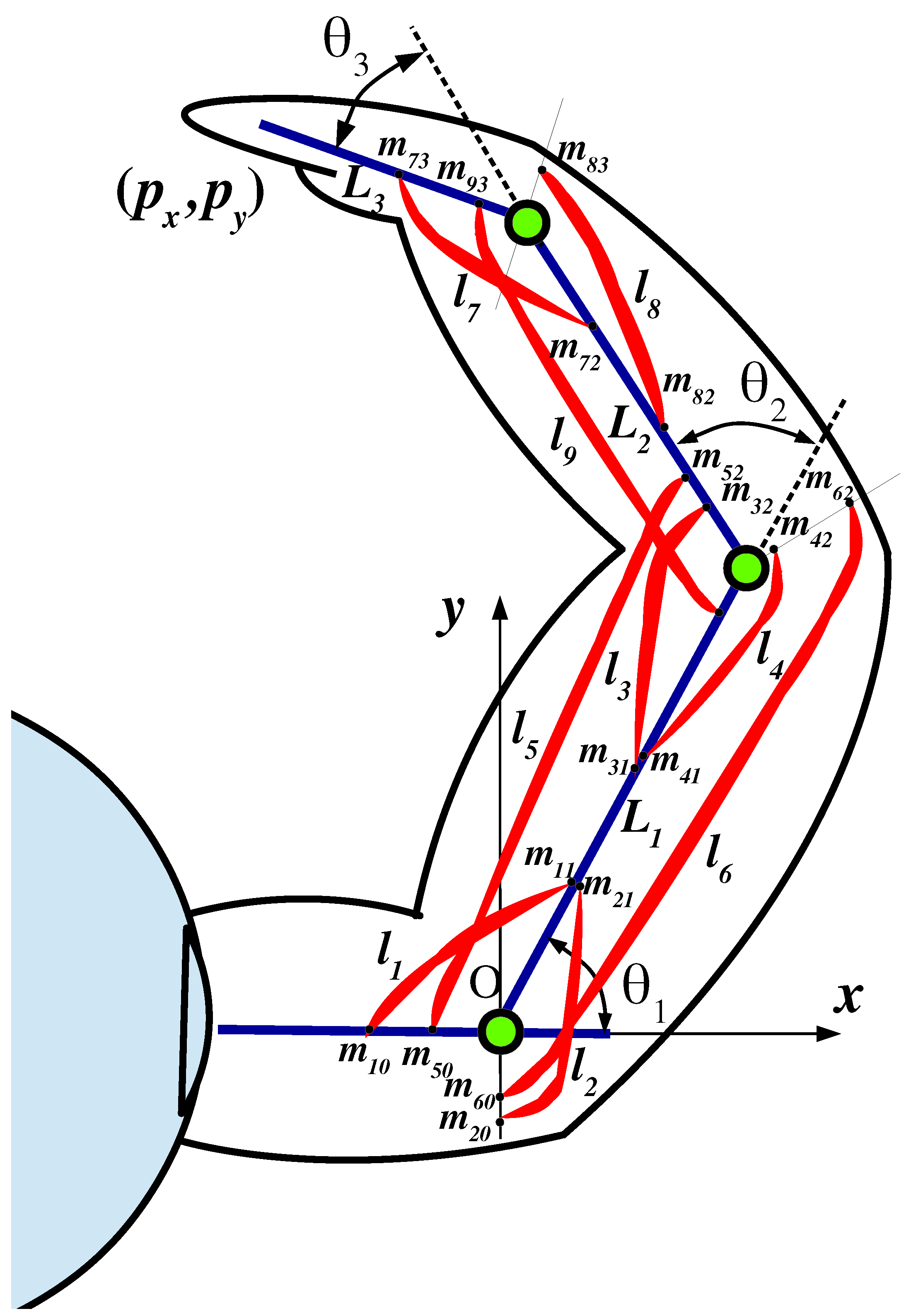
2.1. Relation between Task and Joint Space

The proposed musculoskeletal model has three biarticular and six monoarticular muscles in a curved arrangement and a structure of three links, as shown in Figure 1. We define the end-point arm position $p={[p_x,p_y]}^{\mathsf{T}}\in {\mathbb{R}}^2$ in terms of the joint variables of the arm $\theta ={[{\theta }_1,{\theta }_2,{\theta }_3]}^{\mathsf{T}}\in {\mathbb{R}}^3$. The coordinates of the end-point p without any orientation are described in Cartesian space as follows:

$$\begin{array}{c}\hfill p=\left[\begin{array}{c}{L}_{1}cos\left({\theta }_1\right)+L_{2}cos({\theta }_1+{\theta }_2)+L_{3}cos({\theta }_1+{\theta }_2+{\theta }_3)\\ L_{1}sin\left({\theta }_1\right)+L_{2}sin({\theta }_1+{\theta }_2)+L_{3}sin({\theta }_1+{\theta }_2+{\theta }_3)\end{array}\right]\end{array}$$

(1)

where $L_1,L_2$, and $L_3$ denote the lengths of the shoulder, elbow, and wrist links, respectively, ${\theta }_1$ is the shoulder angle relative to the x-axis coordinate, ${\theta }_2$ is the elbow angle in reference to the shoulder, and ${\theta }_3$ is the wrist angle with regard to the elbow. By differentiating Equation (1), we establish a relationship between the end-point velocity and the angular velocities of the links as

$$\begin{array}{c}\hfill \dot{p}=\mathbf{J}\dot{\theta }\end{array}$$

(2)

where $\mathbf{J}\in {\mathbb{R}}^{2\times 3}$ represents the Jacobian matrix that maps the joint space to the task space, $\dot{p}={[{\dot{p}}_x,{\dot{p}}_y]}^{\mathsf{T}}$ is the end-point linear velocity, and $\dot{\theta }={[{\dot{\theta }}_1,{\dot{\theta }}_2,{\dot{\theta }}_3]}^{\mathsf{T}}$ is the angular velocity. The Jacobian matrix $\mathbf{J}$ is also employed to find the relationship between the joint torques $\tau \in {\mathbb{R}}^3$ and the end-point forces in task space $F\in {\mathbb{R}}^2$ as

$$\begin{array}{c}\hfill \tau ={\mathbf{J}}^{\mathsf{T}}F.\end{array}$$

(3)

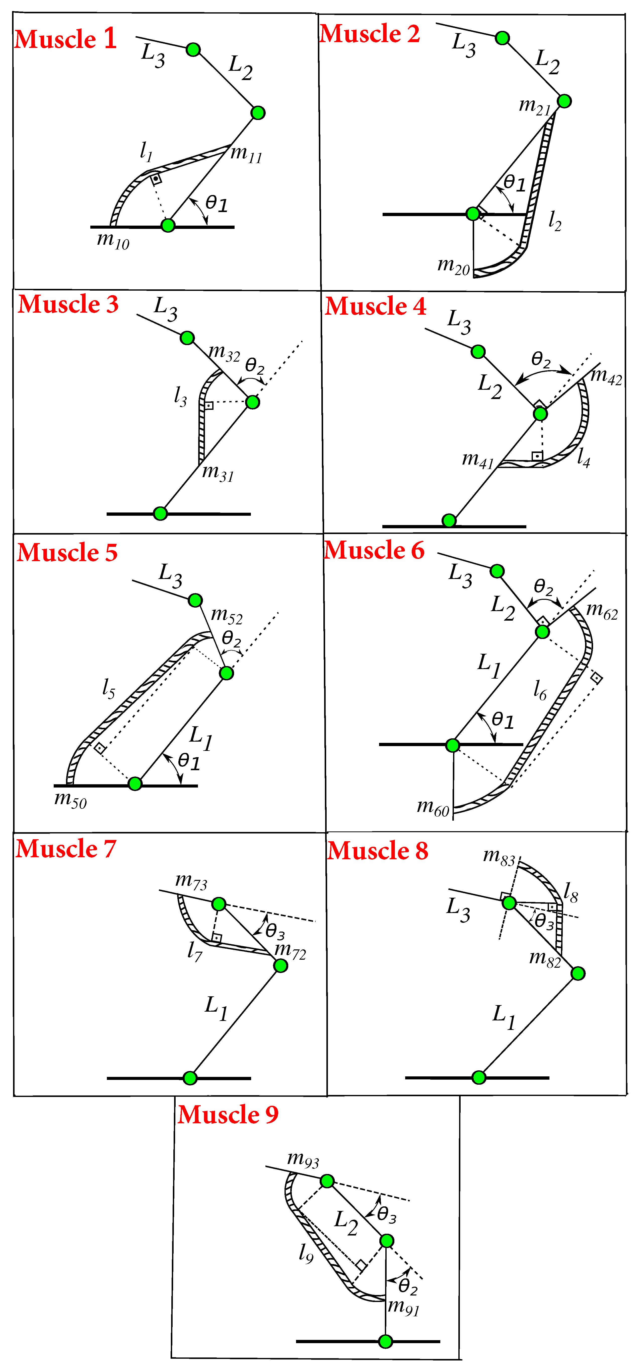
2.2. Relation between Joint and Muscle Space

The proposed musculoskeletal arm (see Figure 1) is transformed into nine possible muscle connections with the rigid links to calculate the i-th muscle length $l_i$ in terms of the joint positions based on the descriptive kinematic analysis (see Figure 2). The existing models often simplify muscle paths as straight lines rather than following curved paths. This study, however, considers that muscles connect to the links via curved paths, providing a more accurate representation of the muscles’ actual anatomical and biomechanical properties.

Figure 2 illustrates the connection of each muscle to the links and allows the muscle length with respect to the reference frame $\left\{O\right\}$ to be calculated using the geometric relationships. Finding the length of each muscle, as shown in Figure 2, requires calculating the angles at which the muscles connect to the links. The muscle length vector $l={[l_1,l_2,\cdots ,l_9]}^{\mathsf{T}}\in {\mathbb{R}}^9$, formulated through the law of cosines, is expressed as:

$$\begin{array}{c}\hfill l=\left[\begin{array}{c}{m}_{10}[\pi -{\theta }_1-arccos\left({\displaystyle \frac{m_{10}}{m_{11}}}\right)]+\sqrt{m_{11}^2-m_{10}^2}\\ m_{20}{\theta }_1+\sqrt{m_{20}^2+m_{21}^2}\\ m_{31}[\pi -{\theta }_2-arccos\left({\displaystyle \frac{m_{31}}{m_{32}}}\right)]+\sqrt{m_{32}^2-m_{31}^2}\\ m_{41}[{\displaystyle \frac{\pi }{2}}+{\theta }_2-arccos\left({\displaystyle \frac{m_{41}}{m_{42}}}\right)]+\sqrt{m_{42}^2-m_{41}^2}\\ m_{50}[{\displaystyle \frac{\pi }{2}}-{\theta }_1]+m_{52}+[{\displaystyle \frac{\pi }{2}}-{\theta }_2]\sqrt{L_1^2+{(m_{50}-m_{52})}^2}\\ m_{60}{\theta }_1+m_{62}{\theta }_2+\sqrt{L_1^2+{(m_{60}-m_{62})}^2}\\ m_{72}[\pi -{\theta }_3-arccos\left({\displaystyle \frac{m_{72}}{m_{73}}}\right)]\\ m_{82}[{\displaystyle \frac{\pi }{2}}-arccos\left({\displaystyle \frac{m_{82}}{m_{83}}}\right)+{\theta }_3]+\sqrt{m_{83}^2-m_{82}^2}\\ m_{93}({\displaystyle \frac{\pi }{2}}-{\theta }_3)+m_{91}({\displaystyle \frac{\pi }{2}}-{\theta }_2)+\sqrt{L_2^2+{(m_{91}-m_{93})}^2}\end{array}\right]\end{array}$$

(4)

where $m_{\mathrm{ij}}$ denotes the distance between the insertion point of i-th muscle, j-th joint center, i = 5, 6, 9 corresponds to the biarticular muscles, and i = 1–4, 7–8 represents the monoarticular muscles. The model parameter values are presented in

Table 1. The muscle model parameter values based on [29].

# Muscle	Value (m)
$l_1$	$m_{10}=0.055,m_{11}=0.08$
$l_2$	$m_{20}=0.055,m_{21}=0.08$
$l_3$	$m_{31}=0.03,m_{32}=0.12$
$l_4$	$m_{41}=0.03,m_{42}=0.12$
$l_5$	$m_{50}=0.04,m_{52}=0.045$
$l_6$	$m_{60}=0.04,m_{62}=0.045$
$l_7$	$m_{72}=0.035,m_{73}=0.01$
$l_8$	$m_{82}=0.05,m_{83}=0.01$
$l_9$	$m_{91}=0.04,m_{93}=0.01$

and established in [29]. The time derivative of the muscle length vector $\dot{l}={[{\dot{l}}_1,{\dot{l}}_2,\cdots ,{\dot{l}}_9]}^{\mathsf{T}}\in {\mathbb{R}}^9$ results in the following:

$$\begin{array}{c}\hfill \dot{l}={\mathbf{J}}_m\dot{\theta }\end{array}$$

(5)

where ${\mathbf{J}}_m\in {\mathbb{R}}^{9\times 3}$ represents the muscle Jacobian matrix, which maps the angular velocity of the joints $\dot{\theta }={[{\dot{\theta }}_1,{\dot{\theta }}_2,{\dot{\theta }}_3]}^{\mathsf{T}}\in {\mathbb{R}}^3$ to the change rate of the length of muscles $\dot{l}$.

2.3. Muscle Model

This study adopts a muscle model developed by Hill [30] and subsequently refined by [31]. This well-known muscle model calculates the muscle tensile force with the muscle activation level. Muscle length and velocity are the variables employed for precise calculation of the muscle tensile force, and each muscle force $F_{im}$ is found by:

$$\begin{array}{c}\hfill F_{im}={\alpha }_i{f}_{ia}(l_i,v_i)F_{imax}+f_{ip}\left(l_i\right)F_{imax}\end{array}$$

(6)

where $f_{ia}$ and $f_{ip}$ denote active and passive scaling functions, $F_{imax}$ is the maximal isometric muscle force, $v_i$ denotes the muscle length velocity, and ${\alpha }_i\in [0,1]$ indicates the muscle activation level. The contraction at constant length and zero muscle activation (${\alpha }_i=0$), where the velocity of muscle shortening is zero, called the passive muscle force, is calculated from the force–length relationship. The maximum exerted muscle force is generated with ${\alpha }_i=1$ when the force of contraction remains constant, and the velocity of contraction becomes progressively less with regards to the force–velocity relationship. The muscle model is written in a compact form as follows:

$$\begin{array}{c}\hfill F_m={\mathbf{F}}_a\alpha +F_p\end{array}$$

(7)

where ${\mathbf{F}}_a=\mathrm{diag}(F_{a1},\cdots ,F_{a9})\in {\mathbb{R}}^{9\times 9}$ is the active muscle force term, $F_p={[F_{p1},\cdots ,F_{p9}]}^{\mathsf{T}}\in {\mathbb{R}}^9$ is the passive muscle force term, and $\alpha ={[{\alpha }_1,\cdots ,{\alpha }_9]}^{\mathsf{T}}\in {\mathbb{R}}^9$ is the muscle activation vector. The relationship between muscle tensile force $F_m={[F_{1m},F_{2m},\cdots ,F_{9m}]}^{\mathsf{T}}\in {\mathbb{R}}^9$ and joint torques $\tau ={[{\tau }_1,{\tau }_2,{\tau }_3]}^{\mathsf{T}}\in {\mathbb{R}}^3$ is defined as:

$$\begin{array}{c}\hfill \tau ={\mathbf{W}}_m{F}_m\end{array}$$

(8)

where ${\mathbf{W}}_m={\mathbf{J}}_m^{\mathsf{T}}\in {\mathbb{R}}^{3\times 9}$ is transpose of the muscle Jacobian matrix. The number of muscles is larger than the degrees-of-freedom (DoFs) of the link arm, resulting in the infinite admission solutions. The solution can be expressed as follows:

$$\begin{array}{c}\hfill F_m={\left({\mathbf{W}}_m\right)}^{†}\tau +(\mathbf{I}-{\left({\mathbf{W}}_m\right)}^{†}\left({\mathbf{W}}_m\right))\vartheta \end{array}$$

(9)

where ${\mathbf{W}}_m^{†}={\mathbf{W}}_m^{\mathsf{T}}{\left({\mathbf{W}}_m{\mathbf{W}}_m^{\mathsf{T}}\right)}^{-1}\in {\mathbb{R}}^{9\times 3}$ is called the pseudo-inverse matrix of ${\mathbf{W}}_m$, and $\mathbf{I}\in {\mathbb{R}}^{9\times 9}$ is the identity matrix. The first term of Equation (9) defines a minimum two-norm solution vector, and, therefore, the muscle force might be negative. The second term of Equation (9) is an arbitrary vector from the null space of ${\mathbf{W}}_m$, depending on $\vartheta \in {\mathbb{R}}^9$. Equation (9) is rewritten as

$$\begin{array}{c}\hfill F_m={\left({\mathbf{W}}_m\right)}^{†}\tau +\mathbf{N}h\end{array}$$

(10)

where $\mathbf{N}h$ equals an arbitrary muscle force vector that balances the redundant muscles among all the muscles without affecting the end-point pose (internal muscle forces). Thus, the second term represents the internal muscle force generated by the redundant muscles. Note that this term is employed to keep all muscle tensions positive. $\mathbf{N}\in {\mathbb{R}}^{9\times 6}$ represents the null space or kernel of ${\mathbf{W}}_m$, and $h\in {\mathbb{R}}^6$ needs to be determined to ensure that all muscle forces are positive. The problem lies in determining a unique value or values for h under the condition $F_{im}\ge 0\forall i=1,2,\cdots ,9$. Assuming unrestricted joint forces are applied to the muscles to support any arbitrary wrench, the force-closure condition is satisfied when the homogeneous term of ${\mathbf{W}}_m$ remains strictly positive, that is

$$\begin{array}{c}\hfill \forall \mathbf{N}\in \mathit{null}\left({\mathbf{W}}_m\right),\exists \mathbf{N}h\in {\mathbb{R}}_{+}^9.\end{array}$$

(11)

Moreover, muscle forces are bound by both lower and upper limits. Lower force limits ensure muscles remain taut, establishing a minimum stiffness for the arm. Meanwhile, upper force limits prevent extreme muscle deformations. The minimum two-norm solution is employed to select h, minimizing the tensions among all muscles while keeping all muscle forces within bounds. Simply stated:

$$\begin{array}{c}\mathrm{minimize} F_m={\left(\sum _{i=1}^9{F}_{im}^2\right)}^{1/2}\hfill \\ \mathrm{subject} \mathrm{to}\tau ={\mathbf{W}}_m{F}_m \mathrm{and} 0<F_{i,\min }\le F_{im}\le F_{i,\max }\forall i=1,2,\cdots ,9.\hfill \end{array}$$

(12)

The feasible wrenches are those constant static forces/moments applied to the end-point that are balanced by all positive muscle forces, subject to a set of muscle-force limits. To ascertain the feasibility of a wrench balance, we consider the following condition

$$\begin{array}{cc}\hfill \exists & \left\{F_m\right|F_m={\mathbf{W}}_m^{†}\tau +\mathbf{N}h,\mathbf{N}h\in {\mathbb{R}}_{+}^9\}\cap \left\{F_m\right|0<F_{i,\min }\le F_{im}\le F_{i,\max }\forall i=1,2,\cdots ,9\}.\hfill \end{array}$$

This condition affirms the existence of a solution to Equation (10) that intersects the convex set delimited by the muscle-force limits. In essence, this convex set represents a hyperbox in ${\mathbb{R}}_{+}^9$. Substituting Equation (3) into Equation (9), we obtain:

$$\begin{array}{c}\hfill F_m={\left({\mathbf{W}}_m\right)}^{†}{\mathbf{J}}^{\mathsf{T}}F+(\mathbf{I}-{\left({\mathbf{W}}_m\right)}^{†}\left({\mathbf{W}}_m\right))\vartheta .\end{array}$$

(13)

2.4. Robot Dynamics

The dynamic equation of the musculoskeletal model for the three-joint arm in joint space is formulated as

$$\begin{array}{c}\hfill \tau =\mathbf{M}\left(\theta \right)\ddot{\theta }+\mathbf{C}(\theta ,\dot{\theta })\dot{\theta }+G\left(\theta \right)\end{array}$$

(14)

where $\tau ={[{\tau }_1,{\tau }_2,{\tau }_3]}^{\mathsf{T}}\in {\mathbb{R}}^3$ is the joint torque/force vector, $\mathbf{M}\left(\theta \right)\in {\mathbb{R}}^{3\times 3}$ denotes the inertia matrix, $\mathbf{C}(\theta ,\dot{\theta })\in {\mathbb{R}}^{3\times 3}$ represents the vector of centrifugal and Coriolis terms, $\ddot{\theta }={[{\ddot{\theta }}_1,{\ddot{\theta }}_2,{\ddot{\theta }}_3]}^{\mathsf{T}}\in {\mathbb{R}}^3$ is the angular acceleration vector, and $G\left(\theta \right)={[g_1,g_2,g_3]}^{\mathsf{T}}\in {\mathbb{R}}^3$ is the gravity force. In transverse plane motion, the effect of gravity is considered negligible.

3. Control Architecture for Human-Like Arm Movement

3.1. Muscle-Activation

A muscle-activation input, incorporating both the arm and muscle terms, is introduced as follows:

$$\begin{array}{cc}\hfill \alpha =& -{\overline{\mathbf{W}}}_m^{†}{\mathbf{J}}^{\mathsf{T}}\tau +(\mathbf{I}-{\left({\overline{\mathbf{W}}}_m\right)}^{†}\left({\overline{\mathbf{W}}}_m\right))\vartheta \hfill \end{array}$$

where $\alpha$ is the muscle-activation input, ${\overline{\mathbf{W}}}_m={\mathbf{F}}_a{\mathbf{W}}_m$, $\tau ={\mathbf{K}}_{p}e+{\mathbf{K}}_d\dot{e}$, $e=p-p_d$ is the tracking error between p actual position and $p_d\in {\mathbb{R}}^2$ desired position, $\dot{e}=\dot{p}-{\dot{p}}_d$ is the velocity error, ${\mathbf{K}}_p=\mathrm{diag}(k_p,k_p)\in {\mathbb{R}}^{2\times 2}$ denotes the feedback gain of the position where $k_p$ is a scalar constant value, ${\mathbf{K}}_d=\mathrm{diag}(k_v,k_v)\in {\mathbb{R}}^{2\times 2}$ stands for the feedback gain of the velocity where $k_d$ is a scalar constant value, and ${\overline{\mathbf{W}}}_m^{†}$ is the pseudo-inverse matrix of ${\overline{\mathbf{W}}}_m$.

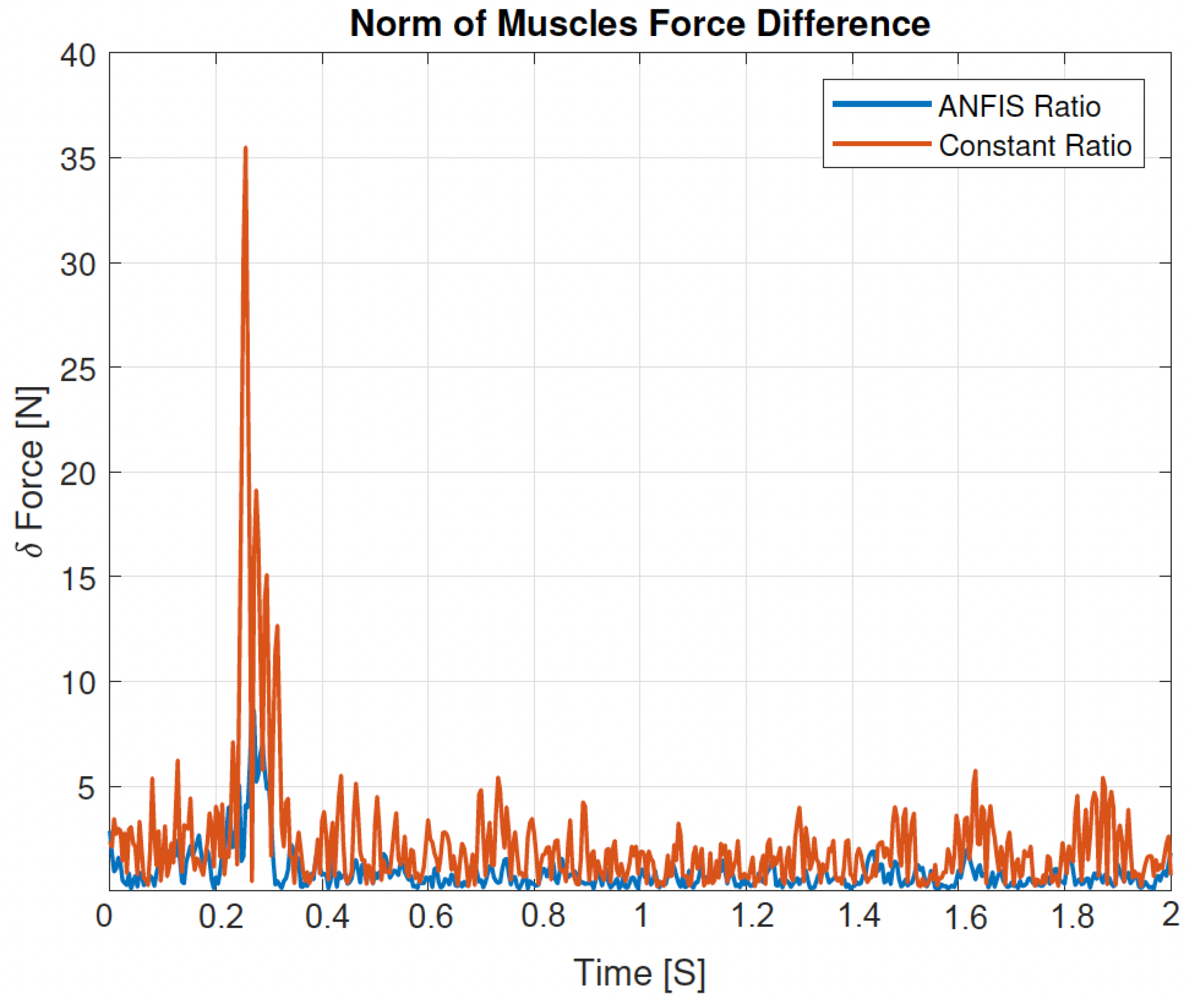
3.2. Muscle-Force Change Cost Function

We introduce a cost function to minimise the difference between muscle forces calculated using the arm movement kinematics and those generated by the control method using muscle activation. Subtracting Equation (9) from Equation (6) yields

$$\begin{array}{cc}\hfill {\displaystyle \underset{\vartheta \in \mathbb{R}}{min}}& E_F\left(\vartheta \right)={\parallel {\mathbf{W}}_m^{†}\tau +({\mathbf{I}}_9-{\mathbf{W}}_m^{†}{\mathbf{W}}_m)\vartheta -{\mathbf{F}}_a\alpha -F_p\parallel }^2\hfill \\ \hfill {\displaystyle \mathrm{subject} \mathrm{to}}& 0\le \alpha \le 1,\hfill \\ & \tau =\mathbf{M}\left(\theta \right)\ddot{\theta }+\mathbf{C}(\theta ,\dot{\theta })\dot{\theta }.\hfill \end{array}$$

(15)

Here, the objective is to minimize $E_F\left(\vartheta \right)={[E_{f1},E_{f2},\cdots ,E_{f9}]}^{\mathsf{T}}\in {\mathbb{R}}^9$ with respect to $\vartheta$. The results of this minimization process are subsequently applied to the following ANFIS structure to identify the null-space parameters, thereby making the motion more human-like.

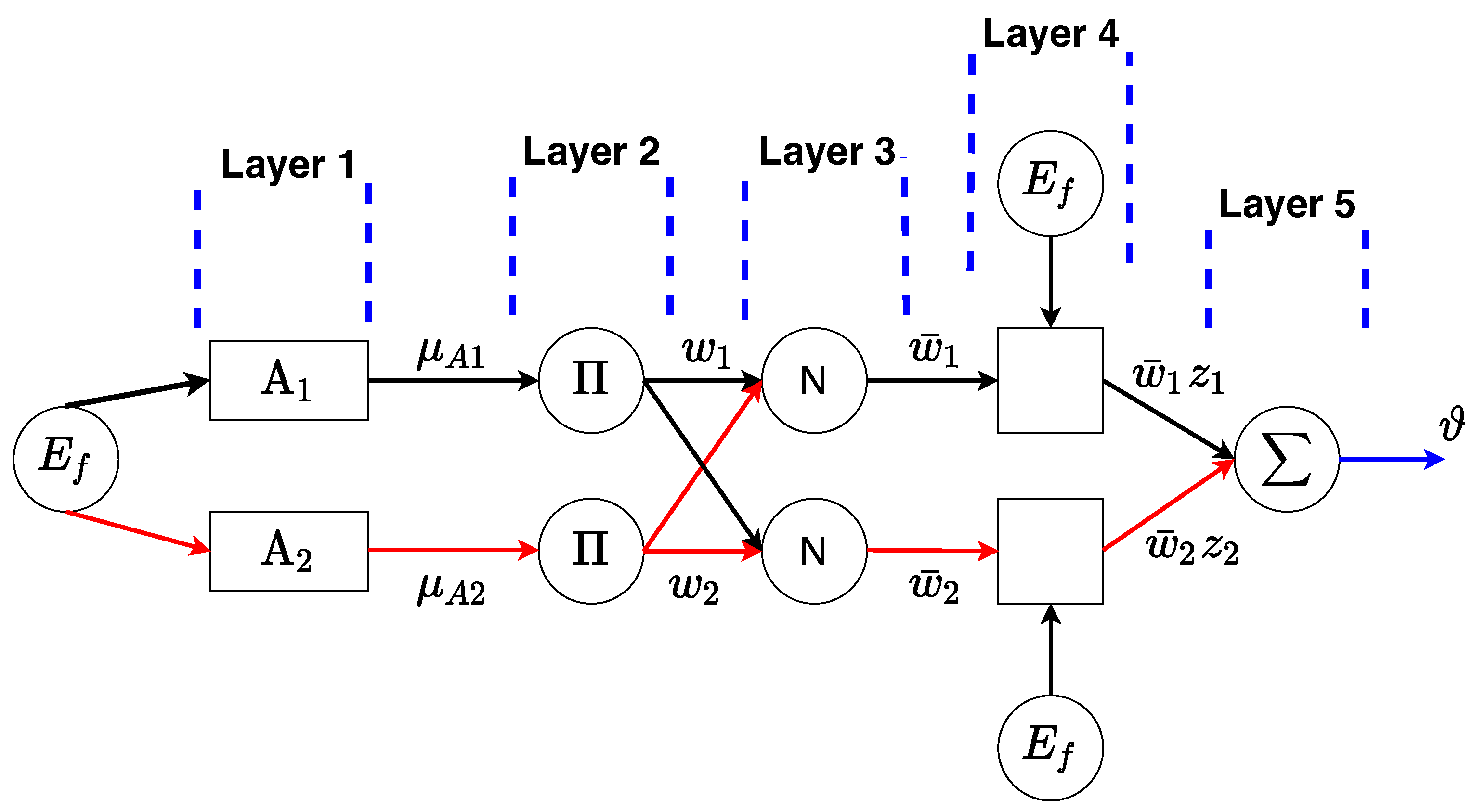
3.3. Adapt the ANFIS Architecture for Human-Like Movement Problem

The proposed ANFIS structure comprises two soft-computing methods: Artificial Neural Network (ANN) and fuzzy logic. A single input variable $E_f$, obtained from the force difference, is selected as the input for the ANFIS. The null-space vector $\vartheta$ is expected to have an output vector of the ANFIS. We express rule sets with a fuzzy if-then rule for the system as

$$\begin{array}{cc}\hfill \mathbf{Rule} \mathbf{1} = \mathbf{IF} E_f \mathrm{is} \mathbf{SMALL},\mathbf{THEN}& \hfill z_1=a_1{E}_f+a_0\\ \hfill \mathbf{Rule} \mathbf{2} = \mathbf{IF} E_f \mathrm{is} \mathbf{LARGE},\mathbf{THEN}& \hfill z_2=b_1{E}_f+b_0\end{array}$$

where $a_0,a_1,b_0$, and $b_1$ are the consequent linear parameters. The proposed ANFIS structure is shown in Figure 3. The ANFIS structure comprises five layers: fuzzy layer, product layer, normalized layer, de-fuzzy layer, and total output layer. The process begins by selecting the input and output variables. For each input variable, fuzzy sets are defined, and fuzzy rules are established for each set. The membership functions of the fuzzy system are then tuned using a hybrid learning algorithm based on neuro-adaptive inference. Finally, the ANFIS model is constructed and trained.

Layer 1 (fuzzy layer): The main function of the first layer is to fuzzify the input variable. Illustrated in Figure 3, the nodes are denoted by squares and labeled $A_1$ and $A_2$. Here, $A_1$ and $A_2$ represent the linguistic labels as SMALL and LARGE, respectively. The node function for each rule is given by

$$\begin{array}{c}\hfill O_{1,1}={\mu }_{A1}\left(E_f\right) \mathrm{and} O_{1,2}={\mu }_{A2}\left(E_f\right)\end{array}$$

(16)

where $O_{1,1}$ and $O_{1,2}$ denote the output functions of each rule, and ${\mu }_{A1}$ and ${\mu }_{A2}$ are the membership functions.

Layer 2 (product layer): This layer’s main role is to calculate the firing strength of each fuzzy rule. The node in this layer performs a multiplication operation on the membership grades received from Layer 1. The nodes are denoted by circles in Figure 3.

$$\begin{array}{c}\hfill O_{2,1}=w_1={\mu }_{A_1} \mathrm{and} O_{2,2}=w_2={\mu }_{A_2}\end{array}$$

(17)

where $w_1$ and $w_2$ denote the firing strength of each rule, respectively.

Layer 3 (normalized layer): The third layer normalizes the firing strengths of the rule obtained from the product layer. The purpose of this layer is to calculate the ratio of the firing strength of the rule to the sum of all rules’ firing strengths, ensuring that the sum of all output signals of this layer equals 1.

The output node is computed based on the proportion between the the rule firing strength and the sum of the firing strengths as

$$\begin{array}{c}\hfill O_{3,1}={\overline{w}}_1={\displaystyle \frac{w_1}{w_1+w_2}} \mathrm{and} O_{3,2}={\overline{w}}_2={\displaystyle \frac{w_2}{w_1+w_2}}\end{array}$$

(18)

where ${\overline{w}}_1$ and ${\overline{w}}_2$ are the normalized firing strengths.

Layer 4 (de-fuzzy layer): The adaptive node function in the fourth layer is described as

$$\begin{array}{c}\hfill O_{4,1}={\overline{w}}_1{z}_1={\overline{w}}_1(a_1{E}_f+a_0) \mathrm{and} O_{4,2}={\overline{w}}_2{z}_2={\overline{w}}_2(b_1{E}_f+b_0)\end{array}$$

(19)

where ${\overline{w}}_1$ and ${\overline{w}}_2$ are from the third layer, $z_1$ and $z_2$ denote the value of the function in the consequent part of each fuzzy rule, and $O_{4,1}$ and $O_{4,2}$ are the outputs of the fourth layer.

Layer 5 (total output layer): The single node in this layer synthesizes the data from the fourth layer and calculates the overall output as

$$\begin{array}{c}\hfill \vartheta =O_5={\overline{w}}_1{z}_1+{\overline{w}}_2{z}_2.\end{array}$$

(20)

In addition, a hybrid learning algorithm comprised of recursive least square (RLS) and gradient descent algorithms is used to estimate the unknown constant parameters in the ANFIS structure. The reader is referred to [32] for the detailed description of the ANFIS architecture.

4. Experimental Design and Materials and Methods

4.1. Participants

The research included the voluntary involvement of 10 subjects who were fully informed and gave their consent before the beginning of any data gathering in accordance with the ethical guidelines of the Helsinki Declaration and with the endorsement of the institution’s ethics committee. The selection of participants was determined by the absence of any recorded visual, motor, or neurological issues.

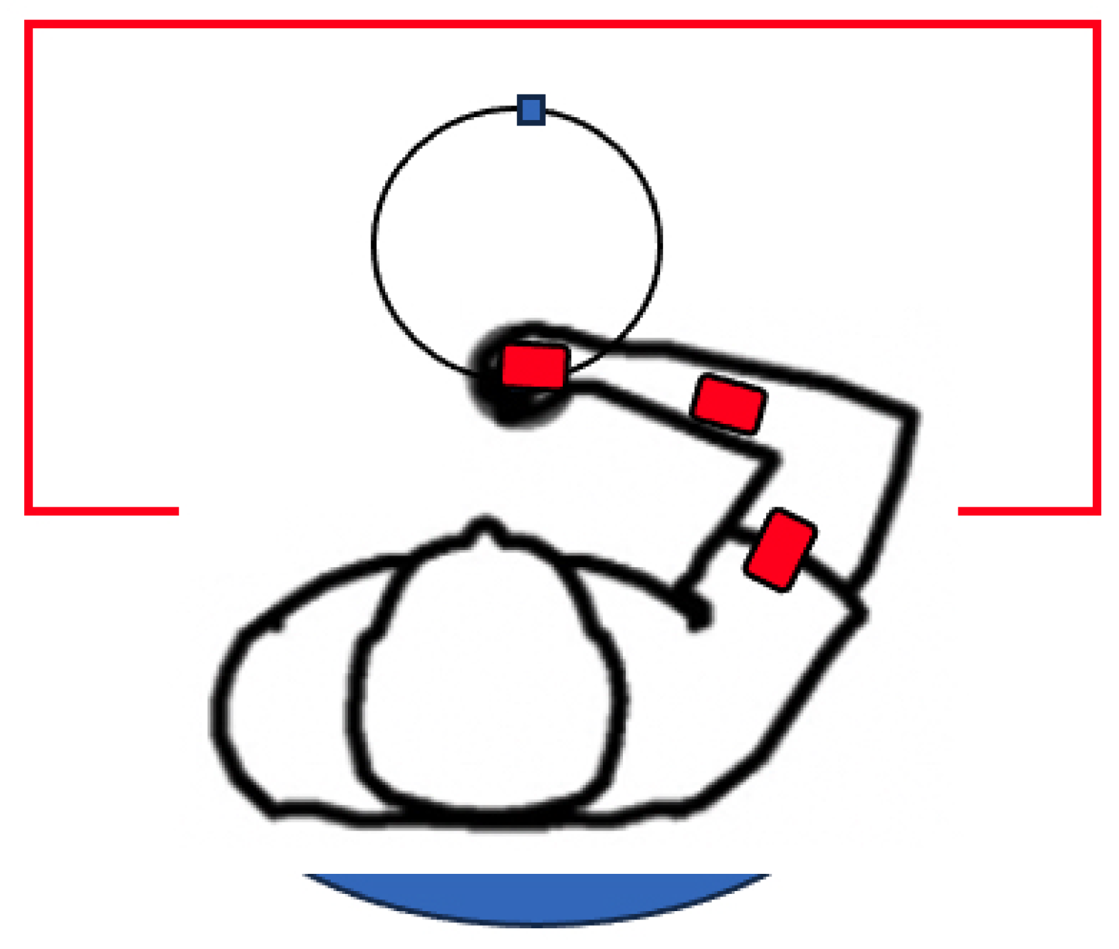
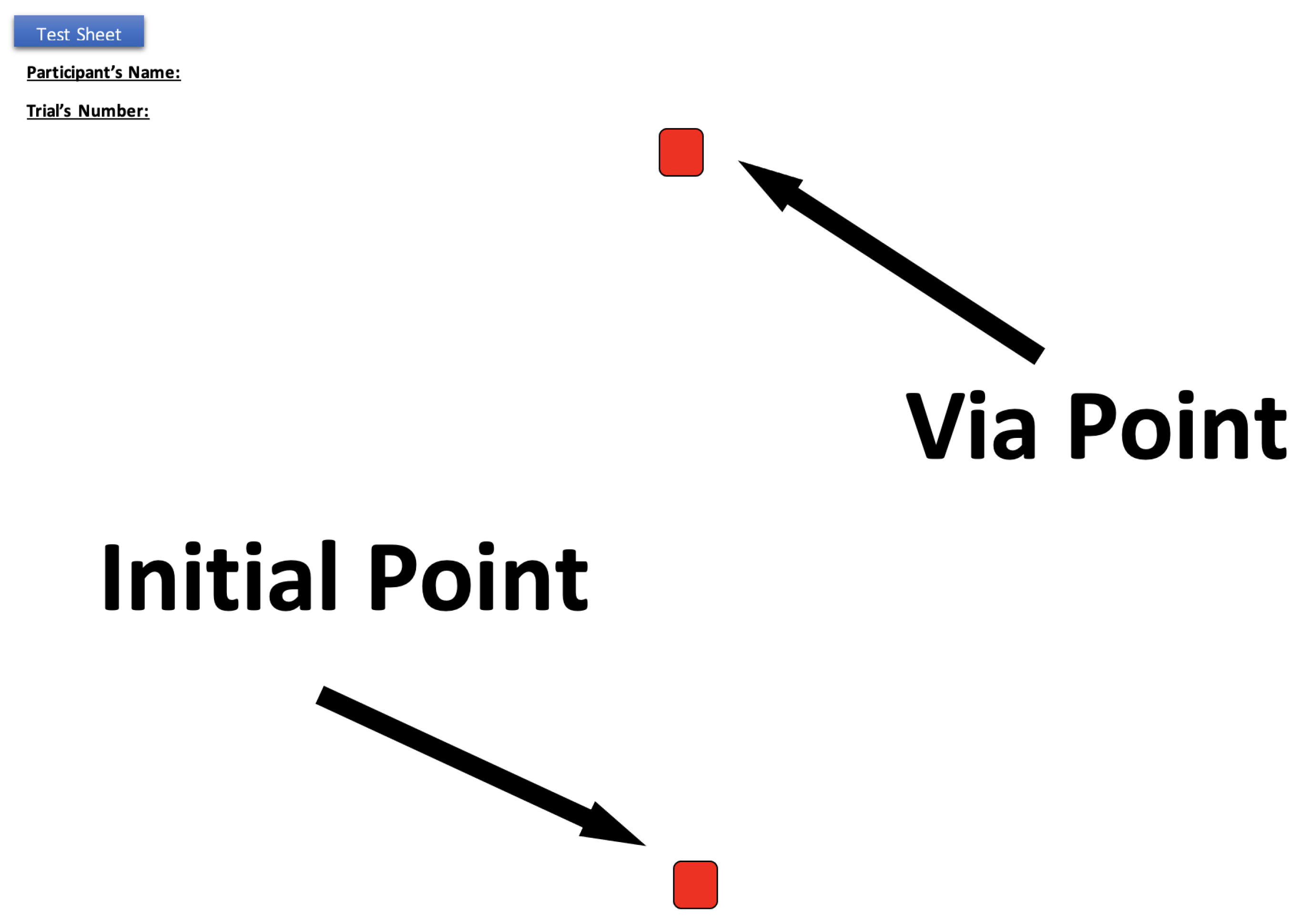
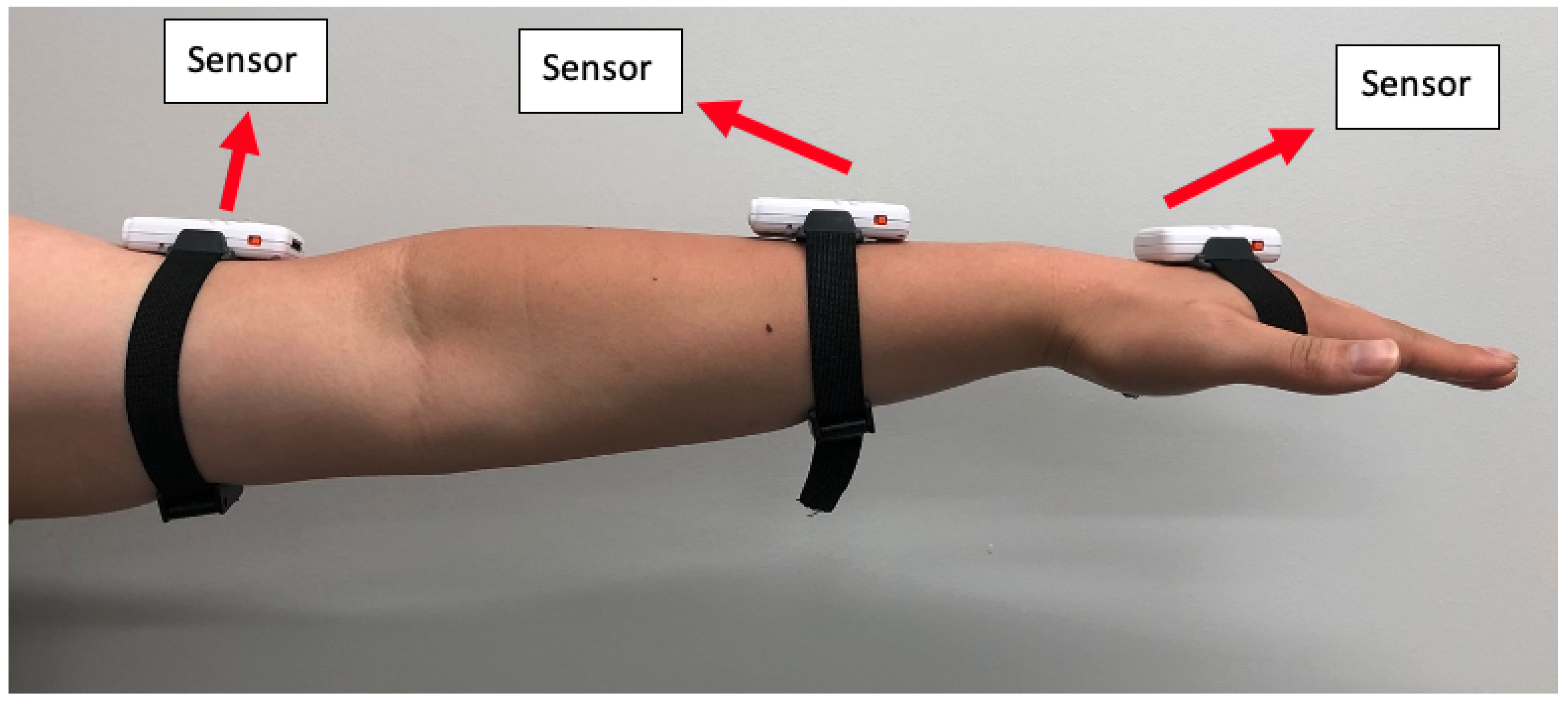
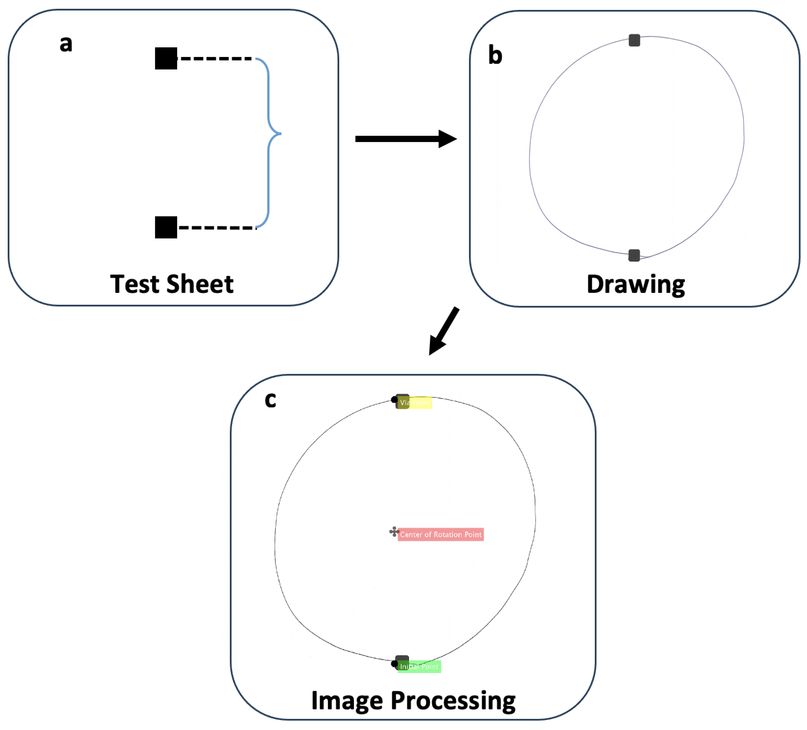
4.2. Setup

The experimental setup used for evaluating the proposed method is depicted in Figure 4. The setup consists of two main parts: image processing and orientation determination. The image processing to capture the movement patterns is initiated once the subjects complete the drawing task on the test sheet (see Figure 5). Following the completion of the drawing, the test sheets are processed using the image analysis to calculate the radius of the drawing. In order to obtain muscle-force difference used for the ANFIS, the orientations of the subjects are recorded via the The inertial measurement unit (IMU) sensors (Shimmer 3) positioned on the subjects’ links, as shown in Figure 6.

To enhance data quality and participant comfort, we place the sensors on the links rather than the joints, driven by the need for stability during measurements, minimizing motion disturbances, and ensuring a consistent sensor orientation. Placing the sensors on the links also mitigates the impact of skin effects associated with joint movement, contributing to adequate signal quality. Additionally, the sensor placement allows for more natural participant movement by avoiding interference with joint motion. Each person is instructed to sit on the same chair with a shoulder-height about 10 centimetres above the experiment table, while the relative distance of the test sheet depends on the length of the person’s arm. The distance is defined to allow the participant to reach the farthest point of the sheet without moving their trunk while they are leaning on the chair. They are instructed to put both hands on the table to avoid stability concentrations. Each participant then completes 10 drawings consisting of large-radius circles (see Figure 7a). The acceptance criteria for a drawing was a maximum time of 2 s to complete the circle.

The task involves using a pen to initiate the circle at the initial point, passing through a designated way point at the farthest position, and finishing by completing the circle by returning to the initial point (see Figure 5 and Figure 7a,b for each step, respectively).

4.3. Methods

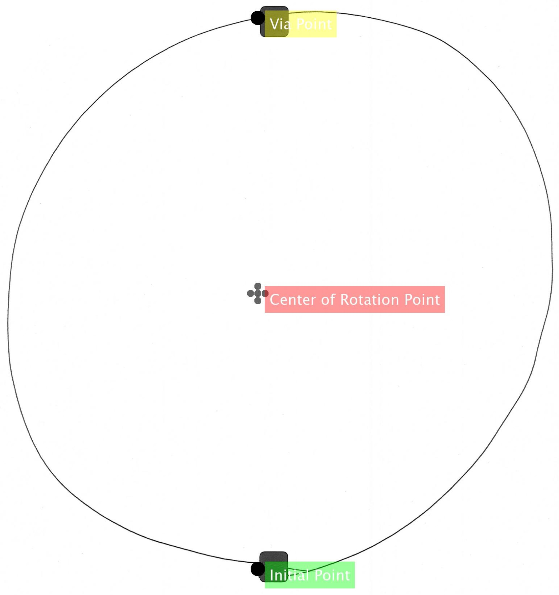
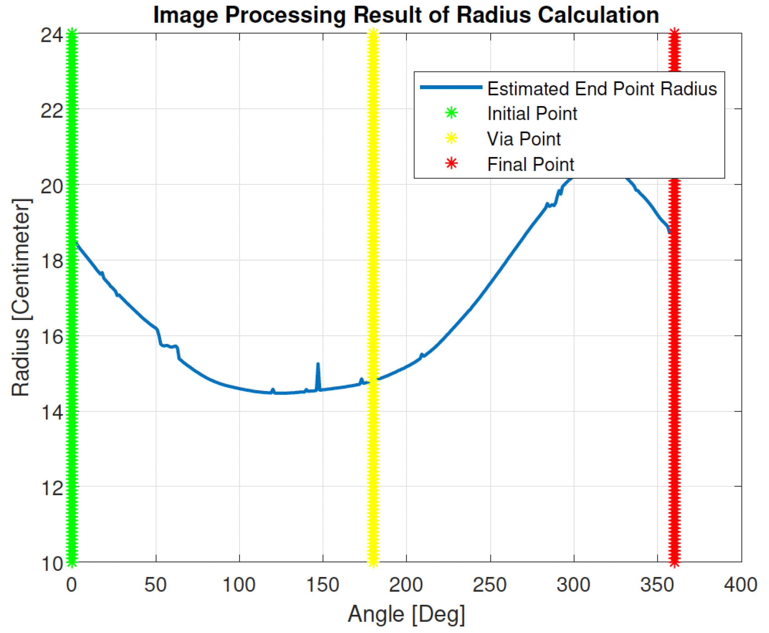
4.3.1. Offline Measurement Method

The proposed offline measurement method is applied after completing all the drawings. The test sheets are scanned using a simple image processing method, and the images are processed in the MATLAB (R2018b) environment. The images are converted to grayscale, and then, using a sharp low pass filter, the dark points are transformed to black while the rest of the image is changed to white (see Figure 7).

In the analysis, the geometric parameters of the drawings are calculated through a systematic image search protocol. The process starts with identifying the cubes within the image, which serve as a reference object to establish scale and define the drawing’s features. The initial and way points of the drawing are pinpointed based on their relative position to the reference cubes. The center of the image is then approximated by calculating the midpoint between the detected initial and way points, thus establishing an arbitrary center for the arc search. Then, utilizing the center, we apply an arc search algorithm across the image to determine the radius of the drawing.

The algorithm examines the image at one-degree intervals around the center, allowing extraction of the radius corresponding to each drawing angle. The method provides the radius of the circle-like drawing as a function of angle. Finally, a matrix of radii with respect to angles from 0 to 360 degrees is calculated, defining the trajectory of the movement with the origin of the arbitrary center point.

4.3.2. Online Measurement Method

In the online method, the sensors are attached to the middle of the links to capture gyroscope and accelerometer data during the drawing. The measurements are then investigated using selective orientation corrections with accelerometers. The measurement data include gyroscope and accelerometer data. The data recording is performed at a frequency of 51.6 samples per second for each tree accelerometer and tri-gyroscope. The initial orientations are calculated as follows:

$$\begin{array}{c}\hfill V\left(0\right)=-a\left(0\right)\times Z\end{array}$$

where V is a horizontal vector of the body frame to reference transformation rotation, Z defines an arbitrary gravity attitude vector in z-axis, a is the initial acceleration vector, and j denotes the time. Sign × denotes the standard cross product. The initial orientation vector $\Omega$ is then updated as follows:

$$\begin{array}{cc}\hfill \Omega \left(j\right)& =q(j-1)\otimes \left({\displaystyle \frac{\omega \left(j\right)}{f_r}}\right)\otimes q(j-1),\hfill \\ \hfill \Phi \left(j\right)& =\left[\right|\Omega \left(j\right)|,{\Omega }_x\left(j\right),{\Omega }_y\left(j\right),{\Omega }_z\left(j\right)],\hfill \\ \hfill q\left(j\right)& =\Phi \left(j\right)\otimes q(j-1)\hfill \end{array}$$

where q represents the quaternion of the orientation from the body frame to the reference frame, $f_r$ is the measurement frequency, $\omega \left(j\right)$ denotes the angular rotation, $\Phi \left(j\right)$ is the rotation quaternion of the body frame, and ⊗ represents the quaternion product operator. The proposed method computes the orientations estimated through quaternion-based integration of the three-dimensional angular rate of change. The acceleration-based calculation utilizes the same method as the initial orientation definition when $\parallel w\left(j\right)\parallel < {\epsilon }_w$ is satisfied, where ${\epsilon }_w$ represents the minimum angular velocity range, which is set to 0.1 degrees per second.

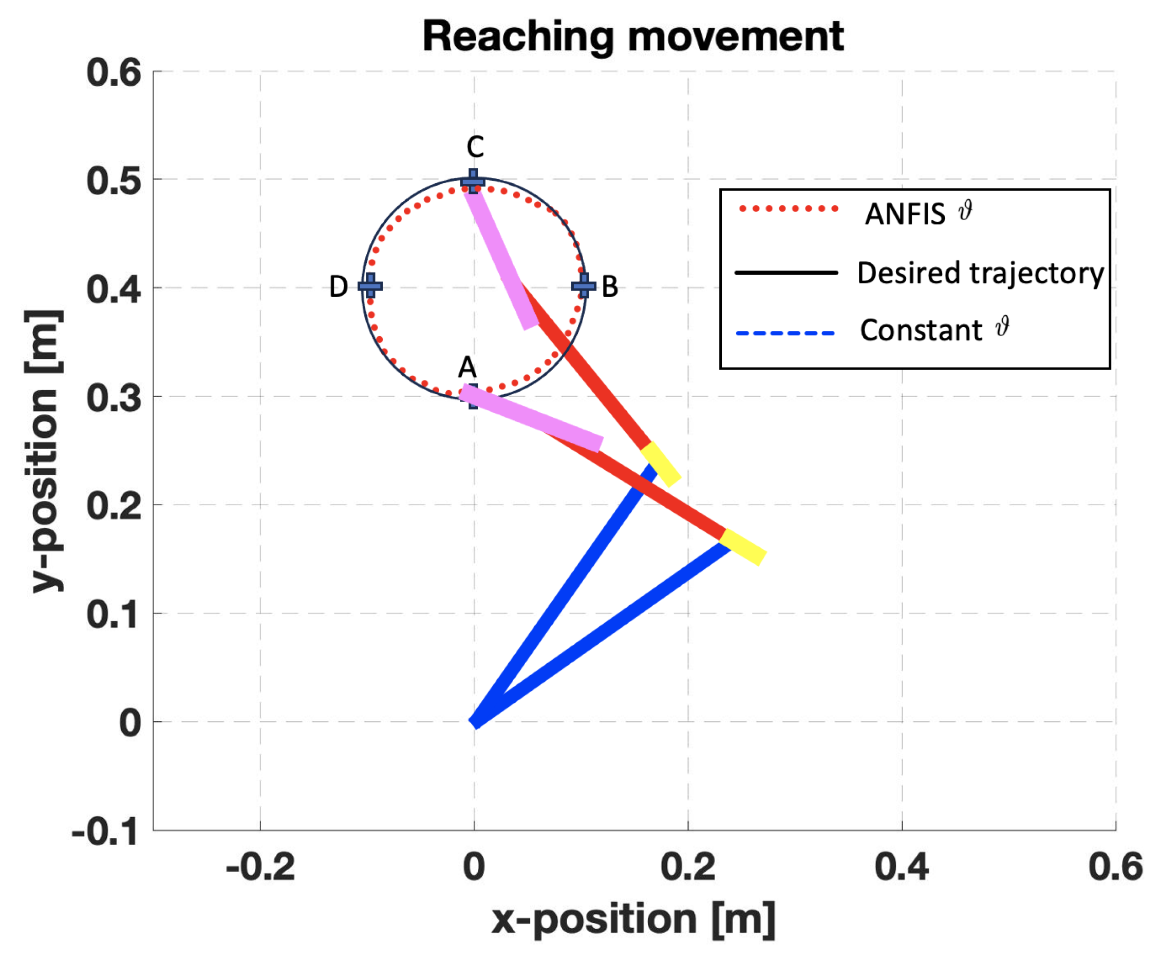
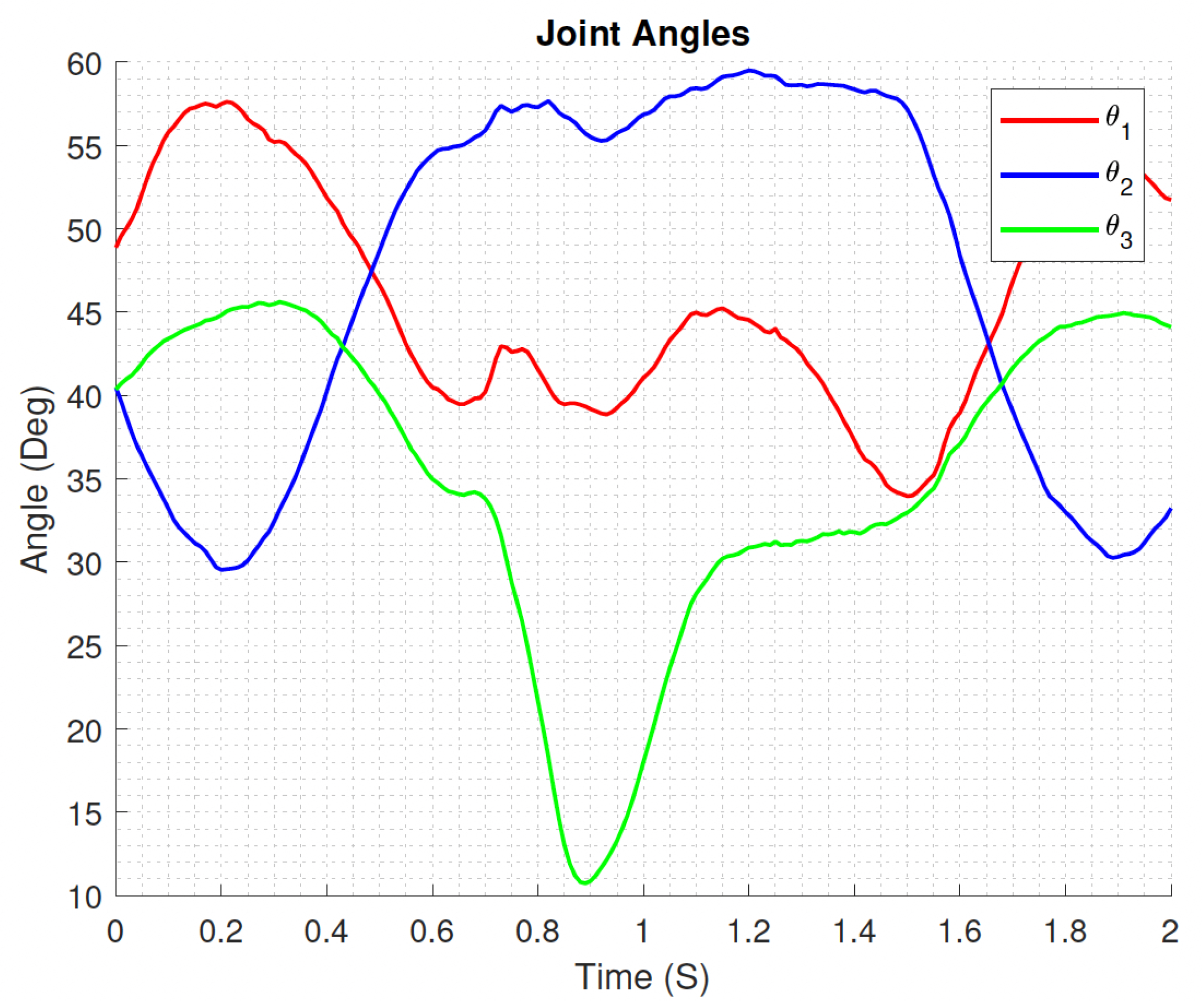
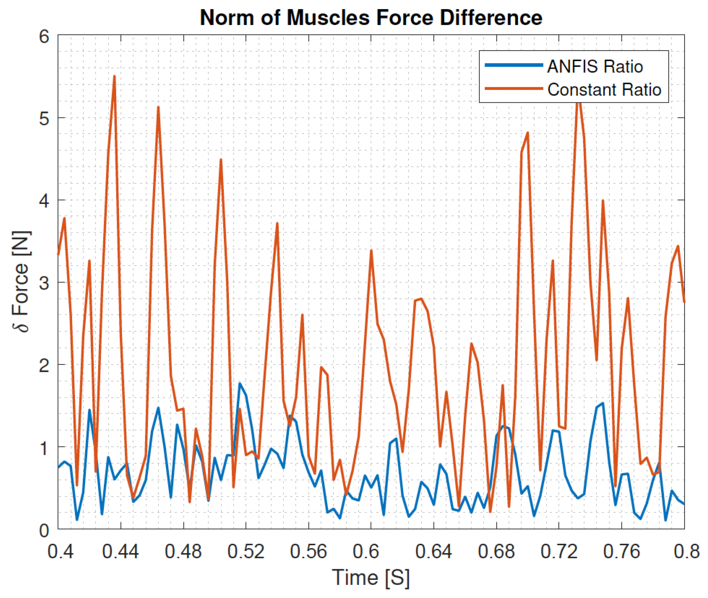
5. Results and Discussion

Measurements

The initial assessment of the subjects’ performance is conducted through the offline image processing methodology. The distribution of the radii of the drawings obtained from the image processing indicates the drawing procedure’s correctness. Verifying that the subject radii exhibit a bell-shaped histogram consistently distributed in line with statistical expectations is crucial. Therefore, the image processing results are essential in validating the experimental procedures.

After the participants complete the drawing task, we employ the image processing procedure to identify the circles’ initial, way, and center points. Figure 8 depicts a sample result of the implemented method on the test sheet. The green-colored text designates the initial point, the yellow-colored text indicates the way point, and the center of rotation, shown in red, represents the midline point location. Subsequently, the extracted data for the radii of the circle-like drawings are calculated. The results for the sample test are illustrated in Figure 9. The green, yellow, and red lines in Figure 9 signify the circle-like drawing’s starting, way, and final points, respectively.

The next step involves determining the angles of each segment based on the online measurement method. Figure 10 shows a sample recording of the resulting Euler angles from the joint movements during the circle-drawing task. After collecting each joint angle from the subjects, the next step is calculating the force difference using Equation (15) for the ANFIS architecture. The performance of the ANFIS’s force variation is then compared to a scenario where a single constant $\vartheta$ parameter is not trained through the ANFIS.

In our study, we conducted a comparison between the performance outcomes associated with two distinct approaches to determining the internal force parameter within the musculoskeletal arm model. The first approach utilizes the ANFIS to determine the internal force parameter $\vartheta$. The second approach relies on a single, static internal force parameter that was predetermined and remained unchanged throughout the control process.

The comparison results in Figure 11 highlight the performance differences between the two approaches. As Figure 11 shows, the result demonstrates an improvement in more human-like muscle force generation with the ANFIS approach. The variance in muscle force difference when using the constant parameter is 2.692, whereas the ANFIS method shows a variance of only 0.454. When the variance approaches zero, it indicates that the model provides an accurate and precise approximation. A smaller variance signifies that the predicted values are closely clustered around the mean, having a more reliable and consistent model fit. Therefore, a lower variance in the force difference, as achieved by the ANFIS method, implies a superior and more precise approximation of the human-like muscle force compared to the constant parameter model. For a more detailed examination of the force difference, an enlarged view between 0.4 and 0.8 seconds of Figure 11 is presented in Figure 12.

Moreover, the peak in Figure 11 at approximately 0.2 s is likely associated with the movement initiation in human circle drawing due to biomechanical factors and the motor control involved in such tasks. When the person begins a drawing motion, especially a circular one, there is a need to overcome inertia and start the movement from a static position. The initial burst of force may be required to set the hand in motion, mainly if resistance or the drawing surface offers some friction. In order to evaluate the developed control approach, the musculoskeletal arm model with a circle-type reaching movement is performed. The musculoskeletal arm model is constructed using the framework presented in [29] within the MATLAB environment. The simulation parameters are given in Table 1 and

Table 2. Kinematic and dynamic parameters of the developed arm model based on [29].

	Wrist	Elbow	Shoulder
Inertia (kg·m2)	0.001	0.012	0.141
Mass (kg)	0.35	1.32	1.93
Mass center (m)	0.075	0.135	0.165
Length (m)	0.15	0.27	0.31

.

It should be noted that the proposed method’s efficacy lies in the precision of the underlying muscle model it utilizes. The accuracy of this model is paramount, as it directly influences the reliability and performance of the method in simulating and understanding muscle dynamics and internal force generation. We perform a circle-like reaching movement based on the internal force vector defined in the previous section. To prove the effectiveness of the ANFIS, we compare the performance using ANFIS with that using a single internal force constant (see Figure 11 and Figure 12). The single internal force constant is selected as k = 20. For simplicity’s sake, we define the internal force vector $\mathit{\vartheta }=ku$, where k is a positive constant and $u\in {\mathbb{R}}^9$ is the unit vector. The developed human arm model and the musculoskeletal arm models in the MATLAB environment are presented in Figure 13 and Figure 14, respectively. Figure 15 shows the simulation result of the circle-like reaching movement with feedback constants ${\mathbf{K}}_p$ and ${\mathbf{K}}_d$. It is observed that the end-point smoothly approaches the desired point, and its trajectory is curved in line with the ANFIS. Moreover, when the constant parameter is selected as lower than 20, it can be seen that the trajectory of the end-point exhibits unusual behavior. The ANFIS-based method demonstrates superior adaptability and precision, attributed to its ability to continuously refine the internal force parameter in response to real-time feedback. In contrast, the single internal force parameter approach exhibits limitations in its capacity to adjust to changing dynamics, leading to decreased efficiency and accuracy in the task execution.

6. Conclusions

This study designs and implements a sensorimotor controller that enables a robotic system to mimic human-like circular motion. By optimizing the internal forces of the muscles, we achieve accurate hand trajectory following along the desired path using joint-space feedback. Utilizing the ANFIS structure, we advance the methodology by treating muscle-force parameters as learning variables, allowing for dynamic adjustment based on the muscle’s rate of change. This approach leverages the power of adaptive learning and fuzzy logic to mimic the control of human motor function. The results underscore the effectiveness of the proposed sensorimotor controller, demonstrating improvements in the motion performance. Future work will focus on refining the controller’s adaptability and exploring its application in more complex movement patterns and different robotic platforms. Additionally, further investigation into the integration of sensory feedback mechanisms could enhance the system’s responsiveness and versatility, paving the way for more intuitive and lifelike robotic assistance in various applications.

References

- Gulletta, G.; Erlhagen, W.; Bicho, E. Human-like arm motion generation: A Review. Robotics 2020, 9, 102. [Google Scholar] [CrossRef]
- Breazeal, C.; Scassellati, B. Robots that imitate humans. Trends Cogn. Sci. 2002, 6, 481–487. [Google Scholar] [CrossRef]
- Robinson, N.; Tidd, B.; Campbell, D.; Kulić, D.; Corke, P. Robotic vision for human–robot interaction and collaboration: A survey and systematic review. ACM Trans. Hum.-Robot Interact. 2023, 12, 1–66. [Google Scholar]
- Pei, S.; Wang, J.; Guo, J.; Yin, H.; Yao, Y. A Human-like Inverse Kinematics Algorithm of an Upper Limb Rehabilitation Exoskeleton. Symmetry 2023, 15, 1657. [Google Scholar] [CrossRef]
- Shin, S.Y.; Kim, C. Human-like motion generation and control for humanoid’s dual arm object manipulation. IEEE Trans. Ind. Electron. 2014, 62, 2265–2276. [Google Scholar] [CrossRef]
- Maroger, I.; Ramuzat, N.; Stasse, O.; Watier, B. Human trajectory prediction model and its coupling with a walking pattern generator of a humanoid robot. IEEE Robot. Autom. Lett. 2021, 6, 6361–6369. [Google Scholar] [CrossRef]
- Burdet, E.; Franklin, D.W.; Milner, T.E. Human Robotics: Neuromechanics and Motor Control; MIT Press: Cambridge, MA, USA, 2013. [Google Scholar]
- Jeong, J.H.; Shim, K.H.; Kim, D.J.; Lee, S.W. Brain-controlled robotic arm system based on multi-directional CNN-BiLSTM network using EEG signals. IEEE Trans. Neural Syst. Rehabil. Eng. 2020, 28, 1226–1238. [Google Scholar] [CrossRef]
- Middleton, F.A.; Strick, P.L. Basal ganglia and cerebellar loops: Motor and cognitive circuits. Brain Res. Rev. 2000, 31, 236–250. [Google Scholar] [CrossRef]
- Wagner, F.B.; Mignardot, J.B.; Le Goff-Mignardot, C.G.; Demesmaeker, R.; Komi, S.; Capogrosso, M.; Rowald, A.; Seáñez, I.; Caban, M.; Pirondini, E.; et al. Targeted neurotechnology restores walking in humans with spinal cord injury. Nature 2018, 563, 65–71. [Google Scholar] [CrossRef]
- Mekki, M.; Delgado, A.D.; Fry, A.; Putrino, D.; Huang, V. Robotic rehabilitation and spinal cord injury: A narrative review. Neurotherapeutics 2018, 15, 604–617. [Google Scholar] [CrossRef]
- Kasukawa, Y.; Shimada, Y.; Kudo, D.; Saito, K.; Kimura, R.; Chida, S.; Hatakeyama, K.; Miyakoshi, N. Advanced equipment development and clinical application in neurorehabilitation for spinal cord injury: Historical perspectives and future directions. Appl. Sci. 2022, 12, 4532. [Google Scholar] [CrossRef]
- Averta, G.; Della Santina, C.; Valenza, G.; Bicchi, A.; Bianchi, M. Exploiting upper-limb functional principal components for human-like motion generation of anthropomorphic robots. J. NeuroEngineering Rehabil. 2020, 17, 63. [Google Scholar] [CrossRef]
- Cesari, P.; Shiratori, T.; Olivato, P.; Duarte, M. Analysis of kinematically redundant reaching movements using the equilibrium-point hypothesis. Biol. Cybern. 2001, 84, 217–226. [Google Scholar] [CrossRef]
- Bernstein, N.A. The problem of the interrelation of coordination and localization. Arch. Biol. Sci. 1935, 38, 15–59. [Google Scholar]
- Khan, N.; Stavness, I. Prediction of muscle activations for reaching movements using deep neural networks. arXiv 2017, arXiv:1706.04145. [Google Scholar]
- Nakada, M.; Zhou, T.; Chen, H.; Weiss, T.; Terzopoulos, D. Deep learning of biomimetic sensorimotor control for biomechanical human animation. ACM Trans. Graph. (TOG) 2018, 37, 1–15. [Google Scholar] [CrossRef]
- Huang, X.; Wu, W.; Qiao, H.; Ji, Y. Brain-inspired motion learning in recurrent neural network with emotion modulation. IEEE Trans. Cogn. Dev. Syst. 2018, 10, 1153–1164. [Google Scholar] [CrossRef]
- Chen, J.; Zhong, S.; Kang, E.; Qiao, H. Realizing human-like manipulation with a musculoskeletal system and biologically inspired control scheme. Neurocomputing 2019, 339, 116–129. [Google Scholar] [CrossRef]
- Arimoto, S.; Sekimoto, M. Human-like movements of robotic arms with redundant DOFs: Virtual spring-damper hypothesis to tackle the Bernstein problem. In Proceedings of the 2006 IEEE International Conference on Robotics and Automation, ICRA 2006, Orlando, FL, USA, 15–19 May 2006; IEEE: Piscataway, NJ, USA, 2006; pp. 1860–1866. [Google Scholar]
- Tahara, K.; Kino, H. Reaching movements of a redundant musculoskeletal arm: Acquisition of an adequate internal force by iterative learning and its evaluation through a dynamic damping ellipsoid. Adv. Robot. 2010, 24, 783–818. [Google Scholar] [CrossRef]
- Tahara, K.; Kuboyama, Y.; Kurazume, R. Iterative learning control for a musculoskeletal arm: Utilizing multiple space variables to improve the robustness. In Proceedings of the 2012 IEEE/RSJ International Conference on Intelligent Robots and Systems, Vilamoura-Algarve, Portugal, 7–12 October 2012; IEEE: Piscataway, NJ, USA, 2012; pp. 4620–4625. [Google Scholar]
- Dong, H.; Mavridis, N. Adaptive biarticular muscle force control for humanoid robot arms. In Proceedings of the 2012 12th IEEE-RAS International Conference on Humanoid Robots (Humanoids 2012), Osaka, Japan, 29 November–1 December 2012; IEEE: Piscataway, NJ, USA, 2012; pp. 284–290. [Google Scholar]
- Dong, H.; Figueroa, N.; El Saddik, A. Muscle force control of a kinematically redundant bionic arm with real-time parameter update. In Proceedings of the 2013 IEEE International Conference on Systems, Man, and Cybernetics, Manchester, UK, 13–16 October 2013; IEEE: Piscataway, NJ, USA, 2013; pp. 1640–1647. [Google Scholar]
- Vatankhah, R.; Broushaki, M.; Alasty, A. Adaptive optimal multi-critic based neuro-fuzzy control of MIMO human musculoskeletal arm model. Neurocomputing 2016, 173, 1529–1537. [Google Scholar] [CrossRef]
- Zhao, L.; Li, Q.; Liu, B.; Cheng, H. Trajectory tracking control of a one degree of freedom manipulator based on a switched sliding mode controller with a novel extended state observer framework. IEEE Trans. Syst. Man Cybern. Syst. 2017, 49, 1110–1118. [Google Scholar] [CrossRef]
- Xiuxiang, C.; Ting, W.; Yongkun, Z.; Wen, Q.; Xinghua, Z. An adaptive fuzzy sliding mode control for angle tracking of human musculoskeletal arm model. Comput. Electr. Eng. 2018, 72, 214–223. [Google Scholar] [CrossRef]
- Qiao, H.; Chen, J.; Huang, X. A survey of brain-inspired intelligent robots: Integration of vision, decision, motion control, and musculoskeletal systems. IEEE Trans. Cybern. 2021, 52, 11267–11280. [Google Scholar] [CrossRef]
- Tahara, K.; Arimoto, S.; Sekimoto, M.; Luo, Z.W. On control of reaching movements for musculo-skeletal redundant arm model. Appl. Bionics Biomech. 2009, 6, 11–26. [Google Scholar] [CrossRef]
- Hill, A.V. The heat of shortening and the dynamic constants of muscle. Proc. R. Soc. London. Ser. B-Biol. Sci. 1938, 126, 136–195. [Google Scholar]
- Zajac, F.E. Muscle and tendon: Properties, models, scaling, and application to biomechanics and motor control. Crit. Rev. Biomed. Eng. 1989, 17, 359–411. [Google Scholar]
- Jang, J.S. ANFIS: Adaptive-network-based fuzzy inference system. IEEE Trans. Syst. Man Cybern. 1993, 23, 665–685. [Google Scholar] [CrossRef]