

Recommendation Algorithm Based on Survival Action Rules


Abstract
1. Introduction
- it is based on a global action model represented by survival action rules,
- recommendations for a specific instance are generated based on the fusion of information contained in the action model,
- the method can be applied to datasets containing numerical as well as categorical attributes,
- the algorithm uses a computationally efficient hill climbing strategy to search recommendations.
2. Related Work
3. Methods
3.1. Basic Notions
3.2. Survival Action Rule Induction
| Algorithm 1 An action rule set induction algorithm for censored data. |
| Require: —a dataset described by attributes A, observation time T, and survival status P—a set of input parameters —a set of stable attributes from the set A Ensure: R—a set of survival action rules
|
| Algorithm 2 Specialization of the action rule in the survival analysis. |
| Require: D—a dataset —a collection of examples that are not yet covered —the minimum number of examples that the new rule must cover — the maximum rule coverage —the maximum percentage of examples that can be covered by both the left and right rules —a set of stable attributes from the set A Ensure: r—the action rule
|
Illustrative Example
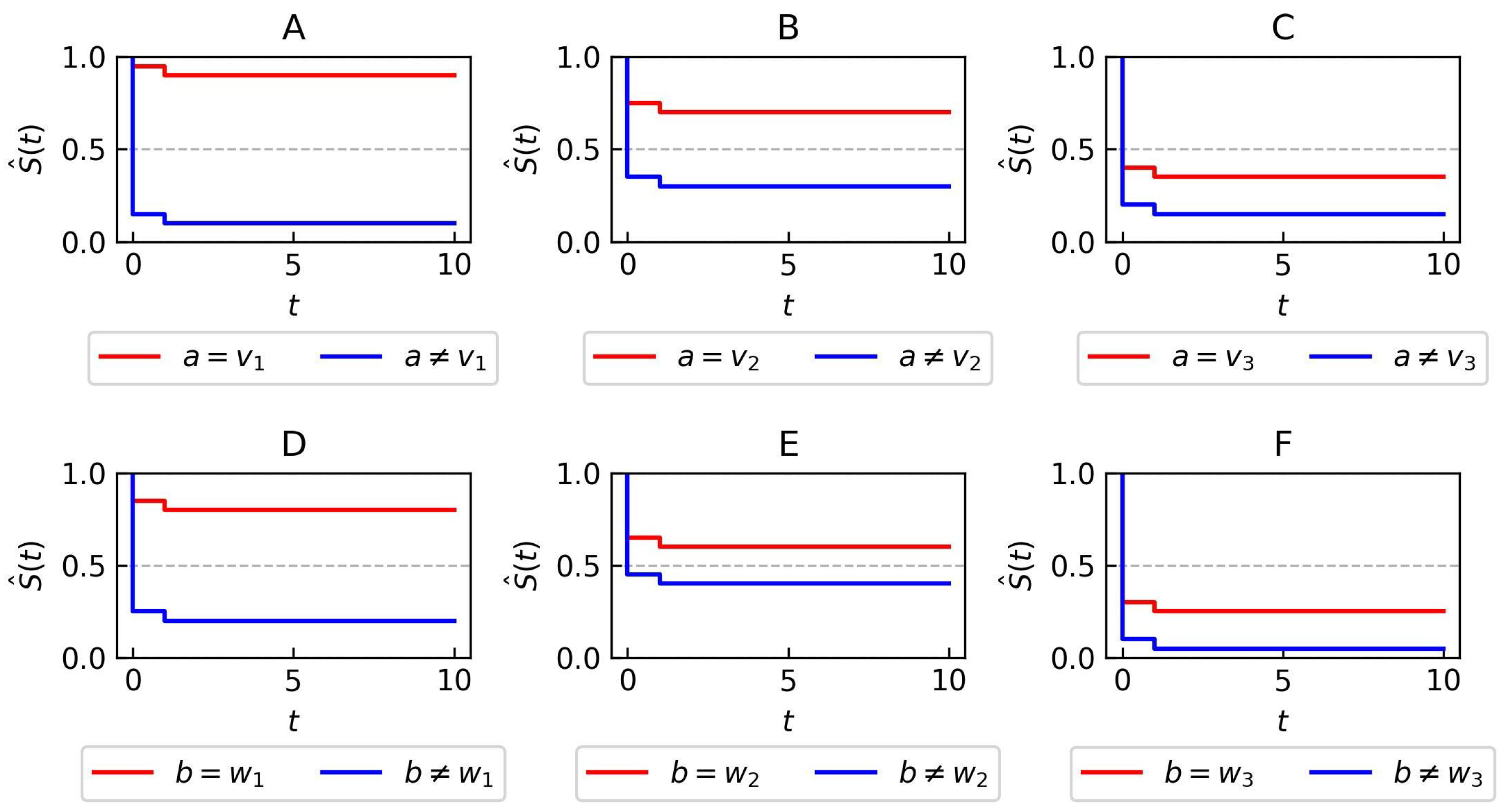
- The initial step involves searching for the best elementary condition to add to the left side of the rule (line 5 in Algorithm 2). In the first iteration, the condition achieves the highest score. This condition is considered the best because it has the largest log-rank test value when comparing the survival curve where with the curve where (panel A in Figure 2).
- The identified elementary condition is then added to the set of previously tested conditions (line 6 in Algorithm 2).
- The best counter-condition is searched for (line 9 in Algorithm 2). In the first iteration, condition achieves the highest score. This condition is considered the best because it has the largest log-rank test value when comparing the survival curve where with the curve where (panels A and C in Figure 2).
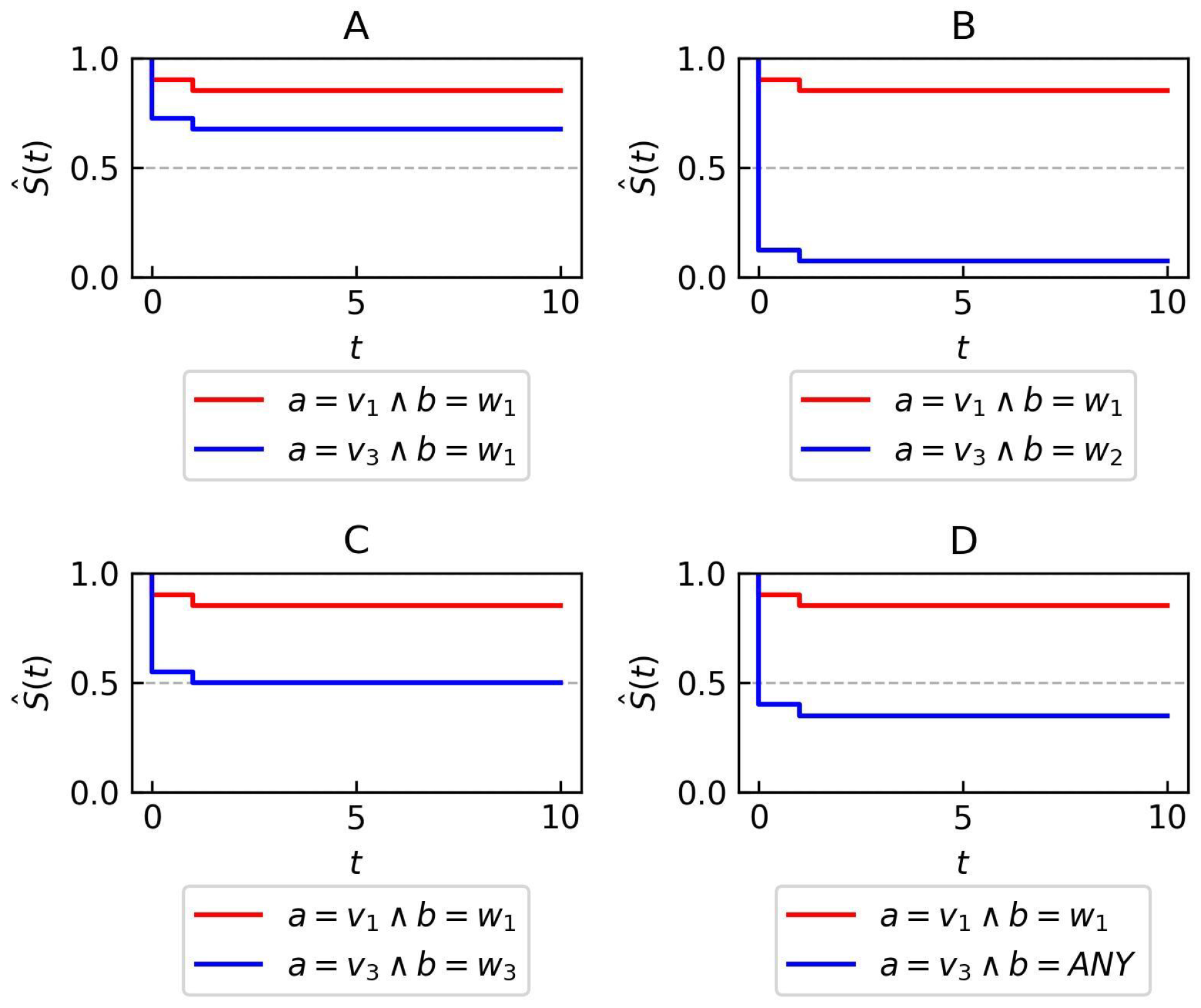
- An action , where denotes the Kaplan–Meier estimate for examples that fulfill the condition , is created from the condition and the counter-condition (line 10 in Algorithm 2). This action is then added to the premise of the rule (line 11 in Algorithm 2).
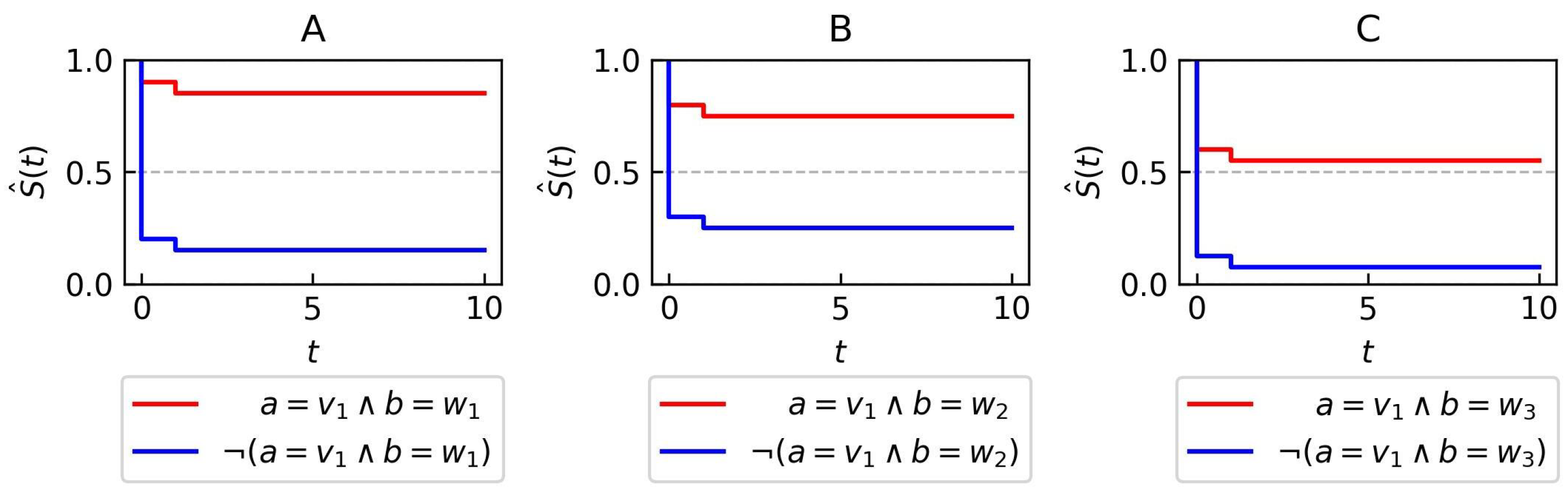
- The initial step involves searching for the best elementary condition to add to the left side of the rule (line 5 in Algorithm 2). In the second iteration, the condition achieves the highest score. This condition is considered the best because it has the largest log-rank test value when comparing the survival curve where with the curve where (panel B in Figure 3).
- The identified elementary condition is then added to the set of conditions previously considered (line 6 in Algorithm 2).
- The best counter-condition is searched for (line 9 in Algorithm 2). In the second iteration, the condition achieves the highest score. This condition is considered the best because it has the largest log-rank test value when comparing the survival curve where with the curve where (panel B in Figure 4).
- An action is created from the condition and counter-condition (line 10 in Algorithm 2). This action is then added to the premise of the rule (line 11 in Algorithm 2).
3.3. Recommendation Induction
3.3.1. Meta-Table
3.3.2. Final Recommendation
4. Experiments and Results
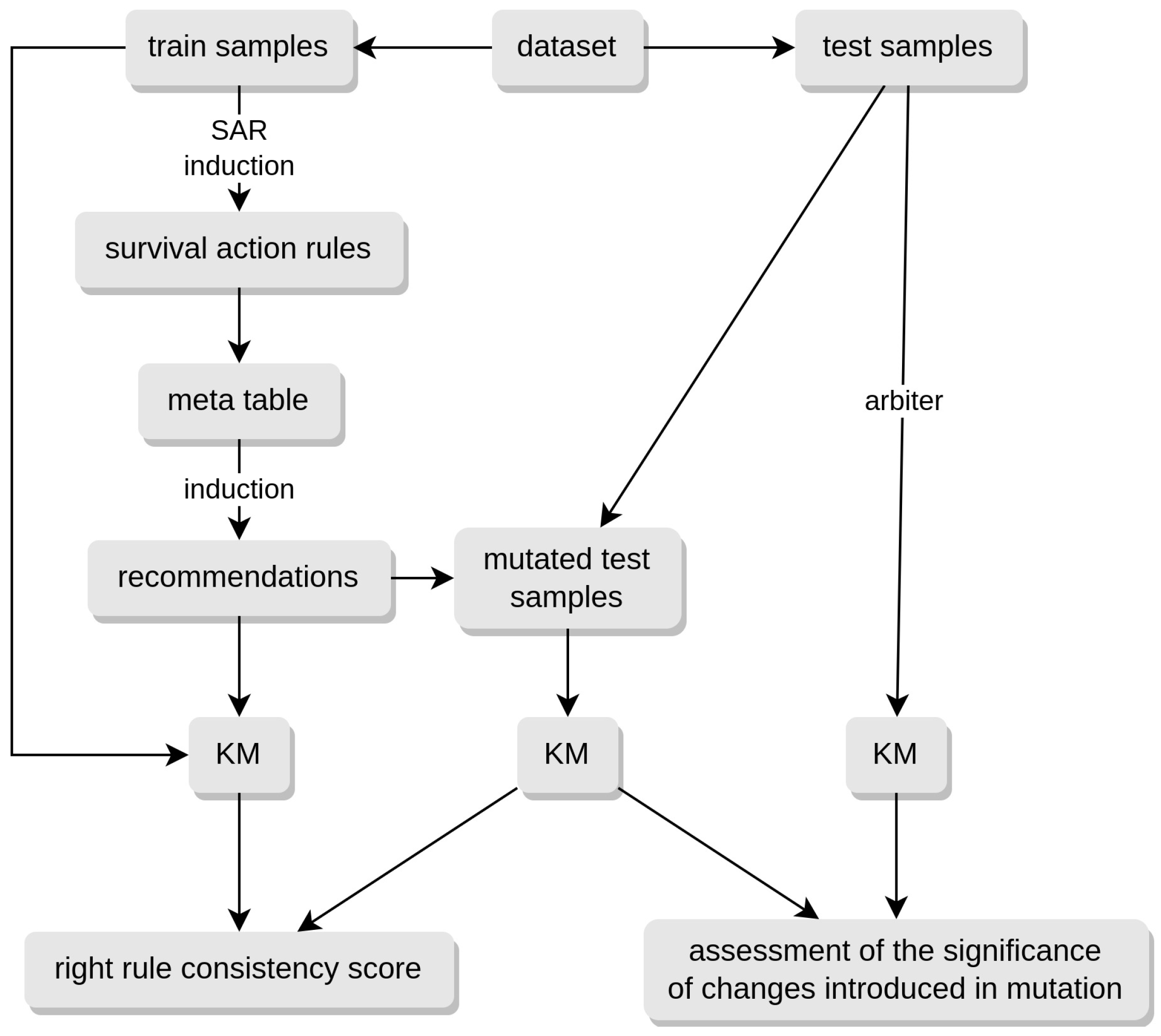
- The XGBoost model is trained on the training data.
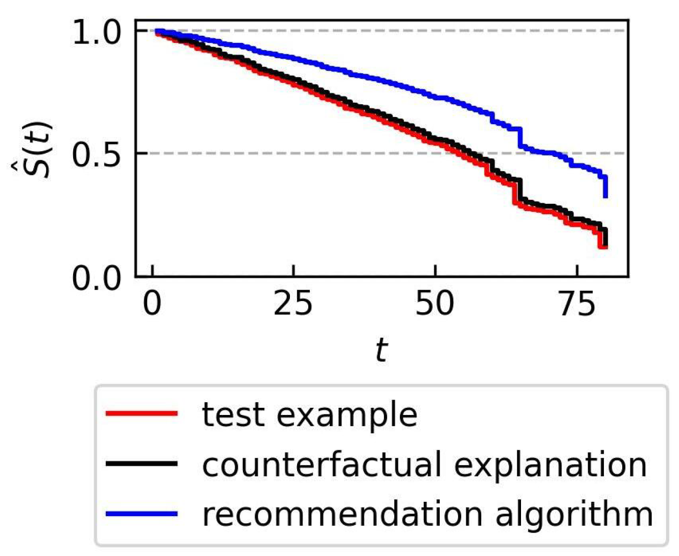
- For each test example x, the survival curve is determined, which represents the conclusion of the recommendation.
- The example is passed to the trained XGBoost model with attribute values modified according to the recommendation algorithm.
- The XGBoost model assigns the survival curve to the example .
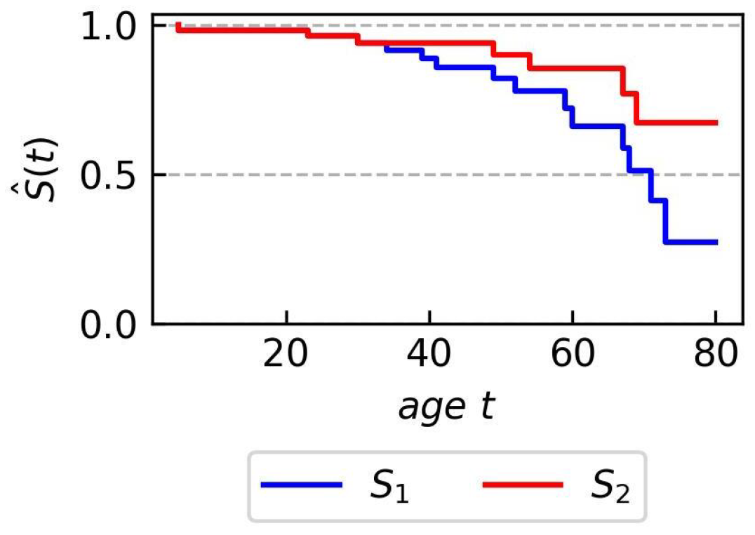
- The difference between the curves and is examined; if the curves are not significantly different, then the rule action model is assumed to be working correctly.
4.1. Case Studies
4.1.1. Maintenance Dataset
- pressureInd
- moistureInd
- temperatureInd
- provider
- team
- time
- status
- number of conditions,
- number of actions,
- the percentage of all examples that the left part of the rule covers,
- the percentage of all examples that the right part of the rule covers,
- p-value of the log-rank test between the Kaplan–Meier curves of the left and right sides of the rule,
- median survival time for examples covered by the left rule (time for probability = ),
- median survival time for examples covered by the right rule,
- difference between the median survival times of the left side of the rule and the right side of the rule.
4.1.2. Comparative Study
Dataset
Detailed Example
5. Conclusions
Author Contributions
Funding
Data Availability Statement
Conflicts of Interest
Abbreviations
| BMI | Body Mass Index |
| CF | counterfactual explanations |
| KM | Kaplan–Meier |
| RUL | survival action rules |
References
- Sikora, M.; Matyszok, P.; Wróbel, Ł. Scari: Separate and conquer algorithm for action rules and recommendations induction. Inf. Sci. 2022, 607, 849–868. [Google Scholar] [CrossRef]
- Badura, J.; Hermansa, M.; Kozielski, M.; Sikora, M.; Wróbel, Ł. Separate-and-conquer survival action rule learning. Knowl.-Based Syst. 2023, 280, 110981. [Google Scholar] [CrossRef]
- Kovalev, M.; Utkin, L.; Coolen, F.; Konstantinov, A. Counterfactual Explanation of Machine Learning Survival Models. Informatica 2021, 32, 817–847. [Google Scholar] [CrossRef]
- Friedman, J.H. Greedy function approximation: A gradient boosting machine. Ann. Stat. 2001, 29, 1189–1232. [Google Scholar] [CrossRef]
- Clark, T.; Bradburn, M.; Love, S.; Altman, D. Survival Analysis Part I: Basic concepts and first analyses. Br. J. Cancer 2003, 89, 232–238. [Google Scholar] [CrossRef] [PubMed]
- Bewick, V.; Cheek, L.; Ball, J. Statistics review: Survival analysis. Crit. Care 2004, 8, 1–6. [Google Scholar]
- Bradburn, M.; Clark, T.; Love, S.; Altman, D. Survival analysis Part II: Multivariate data analysis–an introduction to concepts and methods. Br. J. Cancer 2003, 89, 431–436. [Google Scholar] [CrossRef] [PubMed]
- Kaplan, E.; Meier, P. Nonparametric estimation from incomplete observations. J. Am. Stat. Assoc. 1958, 53, 457–481. [Google Scholar] [CrossRef]
- Harrington, D.; Fleming, T. A class of rank test procedures for censored survival data. Biometrika 1982, 69, 553–566. [Google Scholar] [CrossRef]
- Cox, D. Regression models and life-tables. J. R. Stat. Soc. Ser. B (Methodol.) 1972, 34, 187–220. [Google Scholar] [CrossRef]
- Schober, P.; Vetter, T. Survival analysis and interpretation of time-to-event data: The tortoise and the hare. Anesth. Analg. 2018, 127, 792–798. [Google Scholar] [CrossRef] [PubMed]
- Wang, P.; Li, Y.; Reddy, C.K. Machine learning for survival analysis: A survey. ACM Comput. Surv. (CSUR) 2019, 51, 1–36. [Google Scholar] [CrossRef]
- Segal, M. Regression trees for censored data. Biometrics 1988, 44, 35–47. [Google Scholar] [CrossRef]
- LeBlanc, M.; Crowley, J. Survival trees by goodness of split. J. Am. Stat. Assoc. 1993, 88, 457–467. [Google Scholar] [CrossRef]
- Bou-Hamad, I.; Larocque, D.; Ben-Ameur, H. A review of survival trees. Stat. Surv. 2011, 5, 44–71. [Google Scholar] [CrossRef]
- Wróbel, Ł.; Gudyś, A.; Sikora, M. Learning rule sets from survival data. BMC Bioinform. 2017, 18, 285. [Google Scholar] [CrossRef] [PubMed]
- Sikora, M.; Wróbel, Ł.; Gudyś, A. GuideR: A guided separate-and-conquer rule learning in classification, regression, and survival settings. Knowl.-Based Syst. 2019, 173, 1–14. [Google Scholar] [CrossRef]
- Van Belle, V.; Pelckmans, K.; Van Huffel, S.; Suykens, J. Improved performance on high-dimensional survival data by application of Survival-SVM. Bioinformatics 2011, 27, 87–94. [Google Scholar] [CrossRef] [PubMed]
- Pölsterl, S.; Navab, N.; Katouzian, A. Fast training of support vector machines for survival analysis. In Machine Learning and Knowledge Discovery in Databases; Machine Learning and Knowledge Discovery in Databases. ECML PKDD 2015. Lecture Notes in Computer Science 9285; Springer International Publishing: Cham, Switzerland, 2015; pp. 243–259. [Google Scholar]
- Faraggi, D.; Simon, R. A neural network model for survival data. Stat. Med. 1995, 14, 73–82. [Google Scholar] [CrossRef]
- Ripley, R.; Harris, A.; Tarassenko, L. Non-linear survival analysis using neural networks. Stat. Med. 2004, 23, 825–842. [Google Scholar] [CrossRef]
- Štajduhar, I.; Dalbelo-Bašić, B.; Bogunović, N. Impact of censoring on learning bayesian networks in survival modelling. Artif. Intell. Med. 2009, 47, 199–217. [Google Scholar] [CrossRef]
- Štajduhar, I.; Dalbelo-Bašić, B. Learning bayesian networks from survival data using weighting censored instances. J. Biomed. Inform. 2010, 43, 613–622. [Google Scholar] [CrossRef] [PubMed]
- Ishwaran, H.; Kogalur, U.B.; Blackstone, E.H.; Lauer, M.S. Random survival forests. Ann. Appl. Stat. 2008, 2, 841–860. [Google Scholar] [CrossRef]
- Hothorn, T.; Bühlmann, P.; Dudoit, S.; Molinaro, A.; Van Der Laan, M.J. Survival ensembles. Biostatistics 2005, 7, 355–373. [Google Scholar] [CrossRef] [PubMed]
- Chen, Y.; Jia, Z.; Mercola, D.; Xie, X. A gradient boosting algorithm for survival analysis via direct optimization of concordance index. Comput. Math. Methods Med. 2013, 2013, 873595. [Google Scholar] [CrossRef] [PubMed]
- Shashikumar, S.P.; Josef, C.S.; Sharma, A.; Nemati, S. DeepAISE—An interpretable and recurrent neural survival model for early prediction of sepsis. Artif. Intell. Med. 2021, 113, 102036. [Google Scholar] [CrossRef] [PubMed]
- Hu, S.; Fridgeirsson, E.; Wingen, G.V.; Welling, M. Transformer-Based Deep Survival Analysis. In Proceedings of the AAAI Spring Symposium on Survival Prediction—Algorithms, Challenges, and Applications 2021, Palo Alto, CA, USA, 22–24 March 2021; Volume 146, pp. 132–148. [Google Scholar]
- Fotso, S. Deep neural networks for survival analysis based on a multi-task framework. arXiv 2018, arXiv:1801.05512. [Google Scholar]
- Zhao, L.; Feng, D. Deep neural networks for survival analysis using pseudo values. IEEE J. Biomed. Health Inform. 2020, 24, 3308–3314. [Google Scholar] [CrossRef]
- Ras, Z.W.; Wieczorkowska, A. Action-rules: How to increase profit of a company. In Proceedings of the European Conference on Principles of Data Mining and Knowledge Discovery, Lyon, France, 13–16 September 2000; pp. 587–592. [Google Scholar]
- Tsay, L.S.; Raś, Z. Action rules discovery: System DEAR2, method and experiments. J. Exp. Theor. Artif. Intell. 2005, 17, 119–128. [Google Scholar] [CrossRef]
- Raś, Z.; Tsay, L.S. Mining E-action rules, System DEAR. In Intelligent Information Processing and Web Mining; Data Mining: Foundations and Practice. Studies in Computational Intelligence 118; Springer: Berlin/Heidelberg, Germany, 2008; pp. 289–298. [Google Scholar]
- Agrawal, R.; Srikant, R. Fast algorithms for mining association rules. In Proceedings of the 20th International Conference on Very Large Data Bases—VLDB 1994, Santiago de Chile, Chile, 12–15 September1994; pp. 487–499. [Google Scholar]
- He, Z.; Xu, X.; Deng, S.; Ma, R. Mining action rules from scratch. Expert Syst. Appl. 2005, 29, 691–699. [Google Scholar] [CrossRef]
- Im, S.; Raś, Z. Action rule extraction from a decision table: ARED. In Foundations of Intelligent Systems, Proceedings of the ISMIS 2008, Cosenza, Italy, 3–5 October 2008; Lecture Notes in Computer Science 4994; Springer: Berlin/Heidelberg, Germany, 2008; pp. 160–168. [Google Scholar]
- Matyszok, P.; Wróbel, Ł.; Sikora, M. Bidirectional action rule learning. In Computer and Information Sciences, Proceedings of the ISCIS 2018, Poznan, Poland, 20–21 September 2018; Communications in Computer and Information Science 935; Springer: Cham, Switzerland, 2018; pp. 220–228. [Google Scholar]
- Raś, Z.; Dardzińska, A. Action rules discovery without pre-existing classification rules. In Rough Sets and Current Trends in Computing, RSCTC 2008, Akron, OH, USA, 23–25 October 2008; Lecture Notes in Computer Science 5306; Springer: Berlin/Heidelberg, Germany, 2008; pp. 181–190. [Google Scholar]
- Daly, G.; Benton, R.; Johnsten, T. A multi-objective evolutionary action rule mining method. In Proceedings of the 2018 IEEE Congress on Evolutionary Computation (CEC), Rio de Janeiro, Brazil, 8–13 July 2018. [Google Scholar]
- Hashemi, S.; Shamsinejad, P. Ga2rm: A ga-based action rule mining method. Int. J. Comput. Intell. Appl. 2021, 20, 2150012. [Google Scholar] [CrossRef]
- Bagavathi, A.; Tripathi, A.; Tzacheva, A.A.; Ras, Z.W. Actionable pattern mining-a scalable data distribution method based on information granules. In Proceedings of the 17th IEEE International Conference on Machine Learning and Applications (ICMLA), Orlando, FL, USA, 17–20 December 2018; pp. 32–39. [Google Scholar]
- Benedict, A.C.; Ras, Z.W. Distributed Action-Rule Discovery Based on Attribute Correlation and Vertical Data Partitioning. Appl. Sci. 2024, 14, 1270. [Google Scholar] [CrossRef]
- Tarnowska, K.A.; Bagavathi, A.; Ras, Z.W. High-Performance Actionable Knowledge Miner for Boosting Business Revenue. Appl. Sci. 2022, 12, 12393. [Google Scholar] [CrossRef]
- Yang, Q.; Yin, J.; Ling, C.; Pan, R. Extracting actionable knowledge from decision trees. IEEE Trans. Knowl. Data Eng. 2007, 19, 43–56. [Google Scholar] [CrossRef]
- Subramani, S.; Wang, H.; Balasubramaniam, S.; Zhou, R.; Ma, J.; Zhang, Y.; Whittaker, F.; Zhao, Y.; Rangarajan, S. Mining actionable knowledge using reordering based diversified actionable decision trees. In Proceedings of the International Conference on Web Information Systems Engineering, Shanghai, China, 8–10 November 2016; pp. 553–560. [Google Scholar]
- Su, P.; Yang, J.; Li, Z.; Liu, Y. Mining actionable behavioral rules based on decision tree classifier. In Proceedings of the 13th International Conference on Semantics, Knowledge and Grids (SKG), Beijing, China, 14–15 August 2017; pp. 139–143. [Google Scholar]
- Cui, Z.; Chen, W.; He, Y.; Chen, Y. Optimal action extraction for random forests and boosted trees. In Proceedings of the 21th ACM SIGKDD International Conference on Knowledge Discovery and Data Mining, Sydney, Australia, 10–13 August 2015; pp. 179–188. [Google Scholar]
- Tolomei, G.; Silvestri, F. Generating actionable interpretations from ensembles of decision trees. IEEE Trans. Knowl. Data Eng. 2019, 33, 1540–1553. [Google Scholar] [CrossRef]
- Greco, S.; Matarazzo, B.; Pappalardo, N.; Słowinski, R. Measuring expected effects of interventions based on decision rules. J. Exp. Theor. Artif. Intell. 2005, 17, 103–118. [Google Scholar] [CrossRef]
- Słowiński, R.; Greco, S. Measuring attractiveness of rules from the viewpoint of knowledge representation, prediction and efficiency of intervention. In Proceedings of the International Atlantic Web Intelligence Conference, Lodz, Poland, 6–9 June 2005; pp. 11–22. [Google Scholar]
- Wachter, S.; Mittelstadt, B.; Russell, C. Counterfactual Explanations without Opening the Black Box: Automated Decisions and the GDPR (6 October 2017). Harv. J. Law Technol. 2018, 31, 841–887. [Google Scholar]
- Dandl, S.; Molnar, C.; Binder, M.; Bischl, B. Multi-objective counterfactual explanations. In Proceedings of the International Conference on Parallel Problem Solving from Nature, Leiden, The Netherlands, 5–9 September 2020; pp. 448–469. [Google Scholar]
- Guidotti, R. Counterfactual explanations and how to find them: Literature review and benchmarking. Data Min. Knowl. Discov. 2022. [Google Scholar] [CrossRef]
- Verma, S.; Boonsanong, V.; Hoang, M.; Hines, K.; Dickerson, J.; Shah, C. Counterfactual Explanations and Algorithmic Recourses for Machine Learning: A Review. arXiv 2022, arXiv:2010.10596v3. [Google Scholar]
- Kovalev, M.S.; Utkin, L.V.; Kasimov, E.M. SurvLIME: A method for explaining machine learning survival models. Knowl.-Based Syst. 2020, 203, 106164. [Google Scholar] [CrossRef]
- Chapfuwa, P.; Assaad, S.; Zeng, S.; Pencina, M.J.; Carin, L.; Henao, R. Enabling Counterfactual Survival Analysis with Balanced Representations. In Proceedings of the ACM Conference on Health, Inference, and Learning, New York, NY, USA, 30 March 2021. [Google Scholar]
- Leung, K.M.; Elashoff, R.; Afifi, A. Censoring issues in survival analysis. Annu. Rev. Public Health 1997, 18, 83–104. [Google Scholar] [CrossRef]
- Stevenson, M. An Introduction to Survival Analysis; EpiCentre, IVABS, Massey University: Palmerston North, New Zealand, 2007. [Google Scholar]
- Wohlrab, L.; Fürnkranz, J. A review and comparison of strategies for han1050 dling missing values in separate-and-conquer rule learning. J. Intell. Inf. Syst. 2011, 36, 73–98. [Google Scholar] [CrossRef]
- Hodges, J., Jr. The significance probability of the Smirnov two-sample test. Arkiv Mat. 1958, 3, 469–486. [Google Scholar] [CrossRef]
- Saxena, A.; Goebel, K.F.; Simon, D.L.; Eklund, N.H.W. Damage propagation modeling for aircraft engine run-to-failure simulation. In Proceedings of the International Conference on Prognostics and Health Management, Denver, CO, USA, 6–9 October 2008; pp. 1–9. [Google Scholar]
- Schumacher, M.; Bastert, G.; Bojar, H.; Hübner, K.; Olschewski, M.; Sauerbrei, W.; Schmoor, C.; Beyerle, C.; Neumann, R.; Rauschecker, H.; et al. Randomized 2 x 2 trial evaluating hormonal treatment and the duration of chemotherapy in node-positive breast cancer patients. German Breast Cancer Study Group. J. Clin. Oncol. Off. J. Am. Soc. Clin. Oncol. 1994, 12, 2086. [Google Scholar] [CrossRef] [PubMed]
- Andersen, P.K.; Borgan, O.; Gill, R.D.; Keiding, N. Statistical Models Based on Counting Processes; Springer Science & Business Media: Berlin/Heidelberg, Germany, 2012. [Google Scholar]
- Hosmer, D.W.; Lemeshow, S.; May, S. Applied Survival Analysis: Regression Modeling of Time to Event Data; Wiley-Interscience: Hoboken, NJ, USA, 2008. [Google Scholar]
- Kałwak, K.; Porwolik, J.; Mielcarek, M.; Gorczyńska, E.; Owoc-Lempach, J.; Ussowicz, M.; Dyla, A.; Musiał, J.; Paździor, D.; Turkiewicz, D.; et al. Higher CD34(+) and CD3(+) cell doses in the graft promote long-term survival, and have no impact on the incidence of severe acute or chronic graft-versus-host disease after in vivo T cell-depleted unrelated donor hematopoietic stem cell transplantation in children. Biol. Blood Marrow Transpl. 2010, 16, 1388–1401. [Google Scholar] [CrossRef]
- Pintilie, M. Competing Risks: A Practical Perspective; John Wiley & Sons: Hoboken, NJ, USA, 2006; Volume 58. [Google Scholar]
- Lange, N.; Ryan, L.; Billard, L.; Brillinger, D.; Conquest, L.; Greenhouse, J. Case Studies in Biometry; Wiley Series in Probability and Mathematical Statistics: Applied Probability And Statistics; Wiley: Hoboken, NJ, USA, 1994. [Google Scholar]
- Fotso, S. PySurvival: Open Source Package for Survival Analysis Modeling. 2019. Available online: https://square.github.io/pysurvival (accessed on 26 March 2024).
- Kyle, R.A. ”Benign” monoclonal gammopathy—After 20 to 35 years of follow-up. In Mayo Clinic Proceedings; Elsevier: Amsterdam, The Netherlands, 1993; Volume 68, pp. 26–36. [Google Scholar]
- Fleming, T.R.; Harrington, D.P. Counting Processes and Survival Analysis; John Wiley & Sons: Hoboken, NJ, USA, 2011; Volume 169. [Google Scholar]
- Klein, J.P.; Moeschberger, M.L. Survival Analysis: Techniques for Censored and Truncated Data; Springer Science & Business Media: Berlin/Heidelberg, Germany, 2005. [Google Scholar]
- Abnet, C.C.; Lai, B.; Qiao, Y.L.; Vogt, S.; Luo, X.M.; Taylor, P.R.; Dong, Z.W.; Mark, S.D.; Dawsey, S.M. Zinc concentration in esophageal biopsy specimens measured by x-ray fluorescence and esophageal cancer risk. J. Natl. Cancer Inst. 2005, 97, 301–306. [Google Scholar] [CrossRef]
- Chen, T.; Guestrin, C. XGBoost: A Scalable Tree Boosting System. In Proceedings of the 22nd ACM SIGKDD International Conference on Knowledge Discovery and Data Mining, San Francisco, CA, USA, 13–17 August 2016; pp. 785–794. [Google Scholar] [CrossRef]
- Pratt, J.W.; Gibbons, J.D. Kolmogorov-Smirnov Two-Sample Tests. In Concepts of Nonparametric Theory; Springer: New York, NY, USA, 1981; pp. 318–344. [Google Scholar] [CrossRef]
- Suzuki, E.; Żytkow, J.M. Unified algorithm for undirected discovery of exception rules. Int. J. Intell. Syst. 2005, 20, 673–691. [Google Scholar] [CrossRef]
- Gudyś, A.; Sikora, M.; Wróbel, Ł. RuleKit: A comprehensive suite for rule-based learning. Knowl.-Based Syst. 2020, 194, 105480. [Google Scholar] [CrossRef]


| 1 | 1 | 2 | 2 | 3 | 3 | 4 | 4 | 5 | 5 | |
| 0 | 1 | 0 | 1 | 0 | 1 | 0 | 1 | 0 | 1 |
| Dataset | Miss | Cens | ||
|---|---|---|---|---|
| FD001 [61] | 100 | 24 | 0.00 | 19.00 |
| FD002 [61] | 260 | 24 | 0.00 | 19.69 |
| FD003 [61] | 100 | 24 | 0.00 | 20.00 |
| FD004 [61] | 249 | 24 | 0.00 | 19.76 |
| GBSG2 [62] | 686 | 8 | 0.00 | 56.41 |
| melanoma [63] | 205 | 7 | 0.00 | 65.37 |
| actg320 [64] | 1151 | 11 | 0.00 | 91.66 |
| bmt-ch [65] | 187 | 35 | 1.24 | 54.55 |
| follic [66] | 541 | 4 | 0.00 | 35.67 |
| hd [66] | 865 | 6 | 0.00 | 50.75 |
| lung [67] | 1032 | 7 | 2.60 | 25.97 |
| maintenance [68] | 1000 | 3 | 0.00 | 19.00 |
| mgus [69] | 241 | 9 | 19.59 | 23.65 |
| pbc [70] | 418 | 17 | 14.54 | 61.48 |
| std [71] | 877 | 21 | 0.00 | 60.43 |
| uis [64] | 575 | 13 | 0.00 | 19.30 |
| whas1 [64] | 481 | 7 | 0.00 | 48.23 |
| whas500 [64] | 500 | 13 | 0.00 | 57.00 |
| zinc [72] | 431 | 55 | 57.17 | 81.21 |
| Dataset | |||||||||
|---|---|---|---|---|---|---|---|---|---|
| FD001 | 2.0 | 2.45 | 0.15 | 100 | 100 | 34.72 | 36.44 | 1.0 | 1.0 |
| FD002 | 6.8 | 3.05 | 0.39 | 91 | 86 | 24.43 | 26.13 | 3.6 | 3.1 |
| FD003 | 2.0 | 4.00 | 1.30 | 100 | 100 | 35.06 | 41.50 | 1.0 | 1.0 |
| FD004 | 6.5 | 3.49 | 0.79 | 100 | 100 | 28.48 | 29.94 | 3.4 | 3.1 |
| GBSG2 | 13.8 | 3.31 | 0.47 | 100 | 100 | 27.41 | 33.16 | 11.5 | 2.3 |
| melanoma | 3.9 | 2.62 | 0.63 | 100 | 100 | 32.62 | 38.82 | 2.6 | 1.3 |
| actg320 | 18.4 | 4.00 | 1.96 | 99 | 99 | 22.48 | 39.29 | 16.1 | 2.2 |
| bmt-ch | 4.7 | 2.50 | 0.60 | 100 | 100 | 30.63 | 40.34 | 2.9 | 1.8 |
| follic | 7.2 | 1.86 | 0.45 | 98 | 98 | 33.26 | 22.61 | 4.2 | 3.0 |
| hd | 10.1 | 1.22 | 0.21 | 87 | 81 | 22.10 | 40.01 | 8.0 | 2.1 |
| lung | 7.1 | 2.79 | 0.71 | 100 | 100 | 35.59 | 36.49 | 3.5 | 3.6 |
| maintenance | 20.8 | 2.56 | 0.03 | 98 | 91 | 22.27 | 12.10 | 12.7 | 8.1 |
| mgus | 4.1 | 3.27 | 0.91 | 100 | 100 | 31.00 | 21.63 | 2.8 | 1.3 |
| pbc | 6.8 | 2.73 | 0.49 | 100 | 100 | 29.88 | 45.10 | 5.7 | 1.1 |
| std | 15.1 | 4.18 | 2.10 | 100 | 100 | 23.72 | 28.36 | 7.4 | 7.7 |
| uis | 8.0 | 3.49 | 1.55 | 100 | 100 | 26.80 | 45.86 | 7.0 | 1.0 |
| whas1 | 6.9 | 2.52 | 0.07 | 100 | 100 | 27.58 | 34.88 | 4.9 | 2.0 |
| whas500 | 7.9 | 4.33 | 0.43 | 100 | 100 | 29.33 | 33.44 | 6.6 | 1.3 |
| zinc | 6.9 | 2.59 | 0.90 | 67 | 53 | 21.61 | 39.53 | 4.9 | 2.0 |
| Dataset | Cs0.05 | Cs0.01 |
|---|---|---|
| FD001 | 80 | 66 |
| FD002 | 97 | 95 |
| FD003 | 93 | 86 |
| FD004 | 98 | 95 |
| GBSG2 | 100 | 100 |
| melanoma | 100 | 100 |
| actg320 | 96 | 96 |
| bmt-ch | 100 | 100 |
| follic | 100 | 99 |
| hd | 100 | 100 |
| lung | 100 | 100 |
| maintenance | 92 | 84 |
| mgus | 99 | 99 |
| pbc | 100 | 100 |
| std | 100 | 100 |
| uis | 100 | 100 |
| whas1 | 99 | 98 |
| whas500 | 100 | 100 |
| zinc | 100 | 100 |
| Dataset | ||
|---|---|---|
| FD001 | 2.69 | 14.62 |
| FD002 | 2.36 | 21.92 |
| FD003 | 2.92 | 21.54 |
| FD004 | 2.40 | 26.92 |
| GBSG2 | 1.76 | 46.00 |
| melanoma | 2.01 | 42.22 |
| actg320 | 1.36 | 33.08 |
| bmt-ch | 2.36 | 16.76 |
| follic | 1.97 | 45.00 |
| hd | 1.70 | 38.75 |
| lung | 3.35 | 63.33 |
| maintenance | 1.02 | 46.00 |
| mgus | 2.21 | 35.45 |
| pbc | 1.68 | 19.47 |
| std | 3.22 | 49.57 |
| uis | 2.65 | 33.33 |
| whas1 | 1.18 | 42.22 |
| whas500 | 1.82 | 29.33 |
| zinc | 1.29 | 3.51 |
| Number of examples | 900 |
| Minimum number of examples covered by rule | 30 |
| Stable attributes | None |
| Number of rules | 23 |
| Number of rules without any action in premise | 0 |
| Conditions count | 63 |
| Actions count | 63 |
| Average conditions per rule | 2.74 |
| Average actions per rule | 2.74 |
| Percent of examples covered by left and right rules | 66.67 |
| Percent of examples covered by left rule | 94.78 |
| Percent of examples covered by right rule | 67.11 |
| Id | Premise |
|---|---|
| r1 | (pressureInd, [103.79, 143.68) → (-inf, 95.80)) ∧ (temperatureInd, [45.46, 123.85) → [86.05, 106.59)) ∧ (moistureInd, [75.70, inf) → [94.84, inf)) |
| r2 | (pressureInd, [103.79, 135.02) → [75.67, 96.13)) ∧ (temperatureInd, (-inf, 160.28) → (-inf, 106.59)) ∧ (moistureInd, [89.64, inf) → ANY) |
| r3 | (pressureInd, [101.14, inf) → [36.36, 96.13)) ∧ (temperatureInd, [71.62, 116.04) → [86.05, 106.60)) ∧ (moistureInd, [76.57, inf) → [88.97, inf)) |
| r4 | (pressureInd, [100.32, inf) → (-inf, 96.13)) ∧ (temperatureInd, (-inf, 132.94) → (-inf, 106.59)) |
| Id | p | ||||||||
|---|---|---|---|---|---|---|---|---|---|
| r1 | 3 | 3 | 0 | 33.11 | 12.89 | 0.00 | 56.00 | 67.00 | −11.00 |
| r2 | 3 | 3 | 1 | 30.33 | 21.44 | 0.00 | 56.00 | 65.00 | −9.00 |
| r3 | 3 | 3 | 0 | 31.89 | 15.67 | 0.00 | 56.00 | 66.00 | −10.00 |
| r4 | 2 | 2 | 0 | 42.89 | 28.00 | 0.00 | 58.00 | 65.00 | −7.00 |
| Id | Recommendation |
|---|---|
| 73 | (temperatureInd, (79.57, 85.54] → (45.46, 106.14]) ∧ (moistureInd, (106.22, 110.00] → (112.84, 114.75]) |
| 74 | (temperatureInd, (86.82, 106.14] → (85.54, 86.82]) |
| 75 | (temperatureInd, (61.19, 68.84] → (70.81, 160.28]) ∧ (moistureInd, (94.84, 99.71] → (94.21, 94.83]) |
| 76 | (temperatureInd, (106.64, 108.03] → (85.54, 86.82]) |
| PressureInd | MoistureInd | TemperatureInd | Time | Status |
|---|---|---|---|---|
| 57.46 | 104.98 | 100.53 | 12 | 1 |
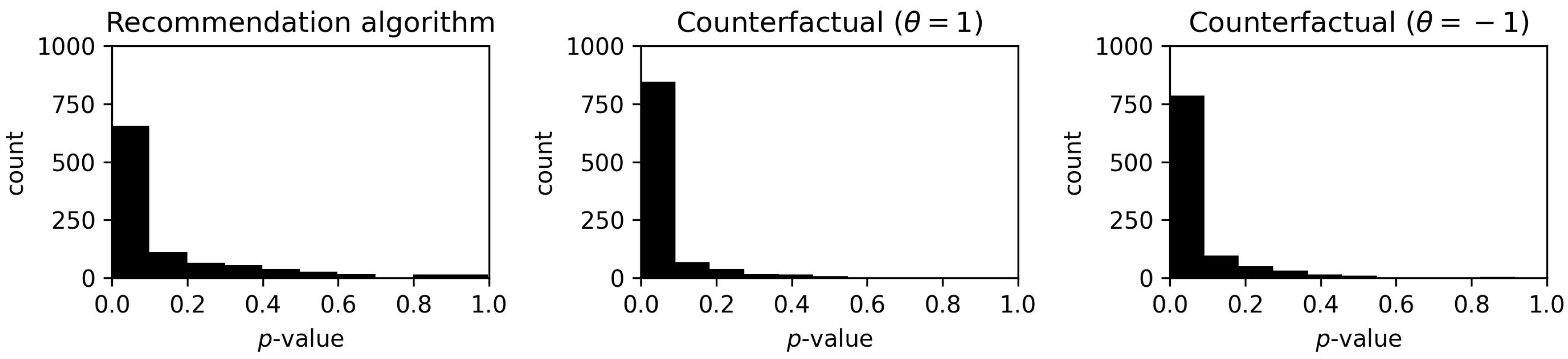
| Method | p-Value ≤ 0.05 |
|---|---|
| recommendation algorithm | 60.8 |
| counterfactuals () | 81.1 |
| counterfactuals () | 74.7 |
| Method | Execution Time |
|---|---|
| recommendation algorithm | 00:03:36 |
| counterfactuals | 03:16:07 |
| ((temperatureInd, (86.82, 106.14) → (temperatureInd, (85.54, 86.82)) |
| PressureInd | MoistureInd | TemperatureInd |
|---|---|---|
| 57.46 | 104.98 | 86.25 |
| PressureInd | MoistureInd | TemperatureInd |
|---|---|---|
| 70.11 | 103.78 | 98.84 |
Disclaimer/Publisher’s Note: The statements, opinions and data contained in all publications are solely those of the individual author(s) and contributor(s) and not of MDPI and/or the editor(s). MDPI and/or the editor(s) disclaim responsibility for any injury to people or property resulting from any ideas, methods, instructions or products referred to in the content. |
© 2024 by the authors. Licensee MDPI, Basel, Switzerland. This article is an open access article distributed under the terms and conditions of the Creative Commons Attribution (CC BY) license (https://creativecommons.org/licenses/by/4.0/).
Share and Cite
Hermansa, M.; Sikora, M.; Sikora, B.; Wróbel, Ł. Recommendation Algorithm Based on Survival Action Rules. Appl. Sci. 2024, 14, 2939. https://doi.org/10.3390/app14072939
Hermansa M, Sikora M, Sikora B, Wróbel Ł. Recommendation Algorithm Based on Survival Action Rules. Applied Sciences. 2024; 14(7):2939. https://doi.org/10.3390/app14072939
Chicago/Turabian StyleHermansa, Marek, Marek Sikora, Beata Sikora, and Łukasz Wróbel. 2024. "Recommendation Algorithm Based on Survival Action Rules" Applied Sciences 14, no. 7: 2939. https://doi.org/10.3390/app14072939
APA StyleHermansa, M., Sikora, M., Sikora, B., & Wróbel, Ł. (2024). Recommendation Algorithm Based on Survival Action Rules. Applied Sciences, 14(7), 2939. https://doi.org/10.3390/app14072939