Analyzing Data Reduction Techniques: An Experimental Perspective

Abstract

The exponential growth in data generation has become a ubiquitous phenomenon in today’s rapidly growing digital technology. Technological advances and the number of connected devices are the main drivers of this expansion. However, the exponential growth of data presents challenges across different architectures, particularly in terms of inefficient energy consumption, suboptimal bandwidth utilization, and the rapid increase in data stored in cloud environments. Therefore, data reduction techniques are crucial to reduce the amount of data transferred and stored. This paper provides a comprehensive review of various data reduction techniques and introduces a taxonomy to classify these methods based on the type of data loss. The experiments conducted in this study include distinct data types, assessing the performance and applicability of these techniques across different datasets.

1. Introduction

The International Data Corporation (mentioned in [1]) estimates that the number of interconnected devices worldwide will exceed 50 billion by 2025. This vast network of devices will generate an impressive volume of approximately 79.4 zettabytes (ZB) of data. As the world becomes increasingly interconnected and data-driven, exploiting the potential of this vast amount of data will play a critical role in driving innovation and enabling progress across multiple sectors.

The proliferation of the Internet of Things (IoT) and a significant increase in Internet-connected devices have resulted in massive amounts of data, commonly known as “Big Data”. Big Data describes heterogeneous and massive datasets that are difficult to analyze and store due to their nature. These datasets contain valuable information that can give companies and organizations a competitive edge. Until 2003, humans had produced 5 exabytes of data; today, the same amount is generated in two days [2]. Big Data poses significant data management challenges, leading recent research to introduce the fundamental “3Vs of Big Data” [3]: volume, velocity, and variety. This paper focuses on the first V, volume, which refers to the massive data size. At the heart of Big Data is the challenge of dealing with massive datasets. These datasets routinely exceed the capacity of traditional databases. The challenge is, therefore, twofold: to effectively manage and store these massive amounts of data while developing efficient processing methods to extract meaningful insights.

Data reduction techniques are essential for optimizing storage, processing, bandwidth consumption, and analysis in Big Data environments. Data reduction involves reducing the size or complexity of data while preserving its essential characteristics and minimizing information loss [4].

Strategically employing data reduction techniques streamlines data transfer and storage processes. The most effective way to perform this task is to implement these techniques in middle servers or gateways, where data can be compressed or aggregated before being sent to the cloud. This approach significantly reduces bandwidth usage and improves efficiency. Alternatively, if energy and computation power are not an issue, data reduction should be applied directly at the sensor level using techniques such as compression or filtering. These techniques offer valuable ways to optimize data handling and improve overall performance.

This paper presents a study and experimental evaluation of various data reduction techniques using different types of datasets to analyze their performance. As part of this research, we also introduce a new taxonomy for data reduction techniques, including lossy and lossless types. By categorizing them based on the data loss characteristics, we provide insights into the trade-offs between data reduction efficiency and the preservation of critical data features. Our experimental evaluation aims to provide a comprehensive understanding of the strengths and limitations of each technique. The main contributions of this work are the following:

• New data reduction techniques’ taxonomies.
• Comparison of different data reduction techniques.
• Experimental evaluation of data reduction techniques.

The rest of this paper is organized as follows: Section 2 provides some background information. Section 3 discusses related work and compares data reduction techniques. Section 4 presents the proposed taxonomy. Section 5 presents the datasets, and the metrics used in the experiments are discussed in Section 6. The data reduction techniques are presented in Section 7, and the experimental evaluation of these techniques is provided in Section 8. Section 9 presents the discussion of the results. Finally, Section 10 focuses on the main conclusions of this study and proposes future work.

2. Background

This section introduces the data reduction concept and the metrics used to evaluate different data reduction techniques.

Data reduction techniques are critical to managing information overload, providing strategic approaches to distill critical insights from massive datasets while containing storage costs [5]. Employing data reduction methodologies such as sampling, aggregation, and dimensionality reduction enables organizations to streamline data analysis processes, making information more accessible in a resource-efficient way. Beyond enhancing scalability, data reduction techniques play a critical role in machine learning, particularly through feature selection, which enables the identification of influential variables, streamlining predictive models for more efficient and accurate decision making. Moreover, reducing data volume addresses the challenge of handling large datasets and directly cuts cloud storage costs. Efficient data management leads to substantial savings, making operations more cost-effective in cloud-based storage solutions.

The following metrics are used in the related work section to study and compare the different data reduction techniques:

• Data size reduction is a percentage-based size comparison of the original and reduced data after applying the reduction techniques.
• Data accuracy quantifies the fidelity of the reduced data to the original dataset, typically expressed as a percentage. This metric measures the integrity and reliability of the reduced dataset, providing insight into the accuracy and fidelity of the information retained by the reduction process.

3. Related Work

Data reduction is a major topic of research in a variety of areas, including Big Data and the Internet of Things (IoT). The fundamental purpose of data reduction strategies is to reduce the storage footprint of a dataset, and this section discusses and summarizes some of the existing work in this area.

Obaise, Salman, and Lafta [6] explored a solution in the IoT gateways that converts time series domains to frequency domains to extract patterns or trends in the streamed data. The solution presented in the paper could reduce cloud storage and bandwidth consumption and prevent I/O bottlenecks. However, the paper did not present the accuracy and reduction percentage, and there is not enough data to calculate it.

Mahmoud, Moussa, and Badr [7] introduced a domain-independent IoT-based spatiotemporal data reduction approach for IoT-structured data, which consists of treating spatial data with the K-Means algorithm to preserve location information and using a data similarity technique on a time basis to preserve temporal data information. The presented solution achieves an average data reduction of 54% with an average accuracy of 95%.

Fathy, Barnaghi, and Tafazolli [8] presented a data reduction technique based on data compression. To reduce the energy consumption when transmitting data to the gateway, the authors proposed an approach in the sensor nodes. The proposed approach consists of two stages: the first stage involves a lossy symbolic aggregate approximation (SAX) quantization stage to minimize the dynamic range of the sensor readings. The final stage is a lossless LZW compression to compress the output of the first stage. The results obtained are a reduction of more than 90% of the produced data, with only 4.74% not reaching the gateway in the worst case. It remains an open possibility to propose a dynamic compression algorithm that can convert from lossless to lossy-based parameters.

Habib et al. [9] present a set of algorithms and techniques to reduce high-volume and high-velocity data in Big Data environments. This survey shows some dimension-reduction approaches to reduce the heterogeneity and massively variable data into manageable data and indicates deduplication techniques and redundancy techniques. It presents a taxonomy of the best and most-used data compression algorithms in terms of decompression overhead. The authors conclude that many efficient data reduction techniques achieve good performance in reduction and accuracy, but they still need more focus from researchers.

Dias, Bellalta, and Oechsner [10] analyzed several prediction-based data reduction approaches to decide which technique is the best to reduce energy consumption in wireless sensor networks. The main contribution was to emphasize not only the introduction of the prediction techniques, but also the methods used in data reduction solutions for WSNs. The authors conclude that the IoT path will depend on the scalability of the sensor networks and their ability to self-access the wireless medium. In addition, the reduction in transmissions based on prediction-based data reduction algorithms depends on the sensed phenomena, the user requirements, and the architecture used to make the predictions.

Chhikara et al. [11] proposed a taxonomy to show the different data dimensionality reduction techniques. The results gathered by the authors with feature extraction techniques show that the best algorithm may vary from data singularities. Principal Component Analysis (PCA), spectral embedding (SE), and uniform manifold approximation and projection (UMAP) were the extraction techniques that gathered the best results in more than one dataset. Among the feature selection techniques, Random Forest and backward feature elimination achieved a reduction percentage of 60%, and the best feature selection technique is forward feature selection, with a reduction percentage of 68%. It was possible to conclude that data dimensionality reduction techniques make it much easier and faster to process and analyze data by machine learning algorithms and human input.

Azar et al. [12] proposed an energy-efficient approach for IoT data collection and analysis. The proposed technique consists of a data compression technique based on a fast error-bounded lossy compressor conducted on the collected data before sending them to the edge layer. Then, after sending the data to the edge, a supervised machine learning technique is applied. The authors’ results proved that the data can be reduced up to 103 times without affecting the data quality. Energy savings are up to 27% after 4 h, and the data accuracy is 98%. The algorithm is better suited for multisensory reading compression. It remains open to try to increase the energy reduction to increase the lifetime of the IoT network.

Papageorgiou, Cheng, and Kovacs [13] created a solution that addresses the two main bottlenecks of the analyzed solutions. The first bottleneck is the inability of time series network-reduction data reduction techniques to make decisions on an item-by-item basis. The other bottleneck is the lack of systems that can apply any data reduction method without heavy reconfiguration or significant delays. Despite the ability of the proposed solution to handle streamed data, it has inferior results when compared to other a posteriori data reduction techniques. Its accuracy may depend on the domain in which it is applied. It remains to further investigate the “streamification” of data reduction techniques and adaptation of data reduction techniques to specific use cases. In addition, the authors do not present the original size of the studied data in the paper.

Hanumanthaiah et al. [14] gather information about compression techniques and design a solution within a node that compresses data using two lossless compression techniques. The author’s concern in designing the method was to create a system that can compress data at a minimal energy cost in low-power devices. The system achieved a compression ratio of 52.67% and a maximum space saving (free space after compression) of 46.1%. However, the paper does not provide detailed information on the type, size, and accuracy of the data examined.

Table 1. Related work data reduction techniques: comparison.

Algorithm	Accuracy	Dataset Size	Reduction Percentage	Reference
Subtractive Clustering Algorithm	NA 1	NA 1	~97%	[6]
Spatiotemporal Data Reduction	95%	843 KB, 960 KB	~54%	[7]
Perceptually Important Points, Sampling, Piecewise Approximation	76.3% to 93.8%	NA 1	~66%	[13]
Run Length Encoding and Delta lossless compression	NA 1	NA 1	~52%	[14]
Pattern System	NA 1	2880 lines	NA 1	[15]
DCT and mixing operation of scrambled image	100%	NA 1	44.16%	[16]
CCSDS and Scalable encryption scheme	100%	NA 1	12.19%	[17]
JPEG XR compression and Block Scrambling	100%	NA 1	60.77%	[18]

¹ Not Available—information not available in the referenced work.

summarizes the comparison between the different data reduction algorithms according to the references.

4. Proposed Taxonomy

Data reduction techniques cover a range of approaches that can vary in their data loss characteristics. For some organizations, the amount of data loss can be a critical factor in their algorithm selection and decision-making processes.

We believe that the taxonomy we present in this section fills a gap in the reviewed literature, namely the lack of a taxonomy that explicitly considers data loss in data reduction strategies [19,20].

The proposed taxonomy, illustrated in Figure 1, provides a structured framework for categorizing data reduction techniques. There are two fundamental levels: the first level focuses on the existence of data loss after the application of data reduction algorithms, and the second level focuses on algorithmic properties. This taxonomy provides a methodological approach to organize and understand the various data reduction techniques. The visual representation of the taxonomy makes it easier for researchers and practitioners to navigate and understand the techniques’ different categories and subcategories. Ultimately, this taxonomy improves the clarity and accessibility of data reduction techniques, facilitating their evaluation and selection for specific data management and analysis purposes.

In the proposed taxonomy, data reduction approaches are divided into two main categories:

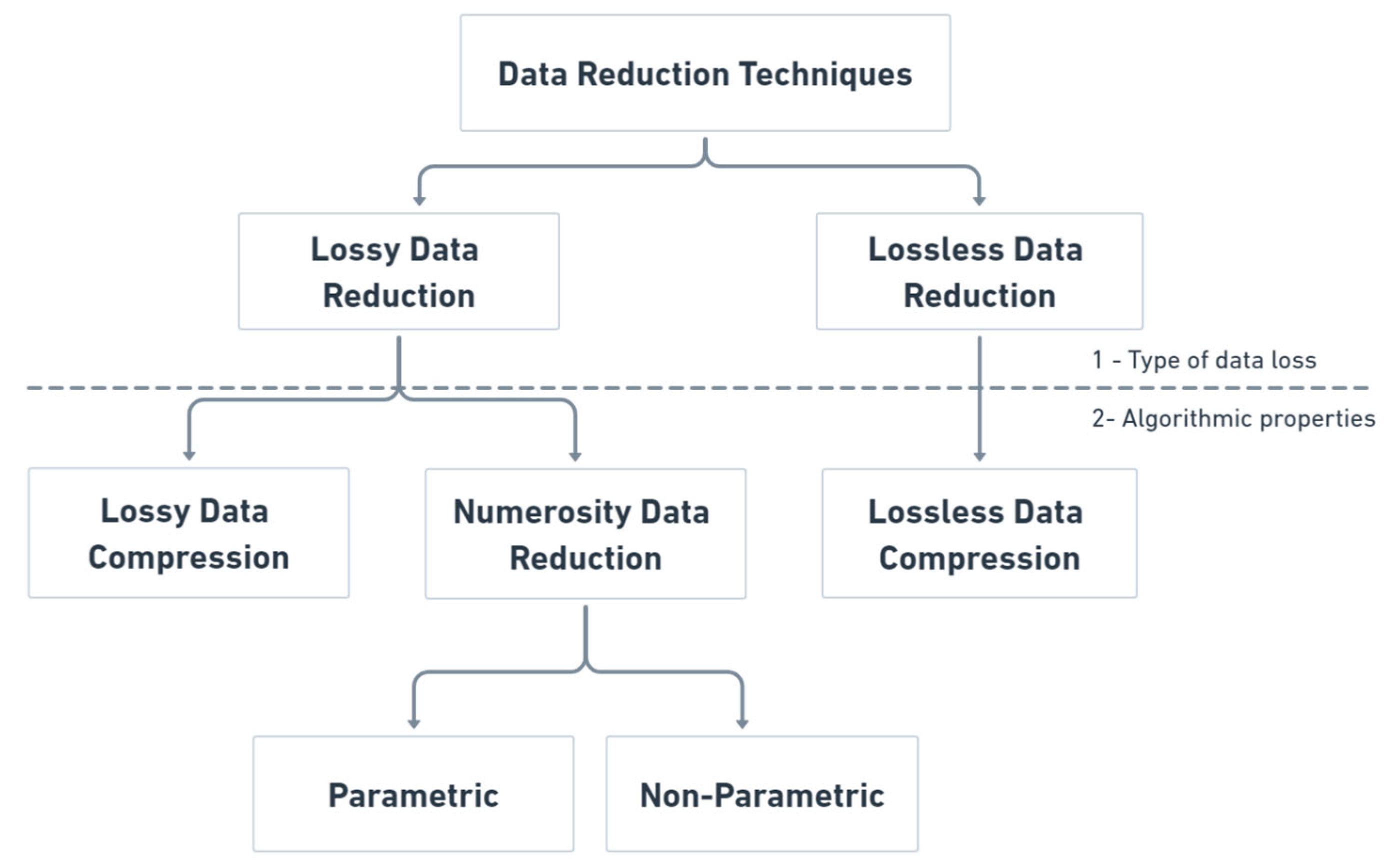
• Lossless data reduction techniques [14,21,22]: these focus on identifying redundancies, patterns, and other inherent characteristics within the data to eliminate or minimize unnecessary and repetitive information. Reducing the data size without any loss is remarkable. However, these algorithms often depend on the type of data they are analyzing. These perform better on repetitive single-sensor data, such as temperature readings. For large-scale datasets, these techniques tend to require a significant processing time to complete the compression, which can be challenging in real-time environments. When time is a primary feature and the workload is enormous and complex, using lossy data reduction algorithms is a viable option. These algorithms include various methods for reducing the data size by selectively discarding or approximating information from the original dataset. Their main advantages include faster processing speeds and the ability to handle a variety of data formats. All these lossless algorithms compress data and can decode the reduced algorithm back to its original size. Some examples of lossless algorithms include Delta Encoding, LZ77, LZ78, Huffman coding, and Run Length Encoding [23,24].
• Lossy data reduction techniques [10,25,26,27]: these focus on reducing data by discarding some details considered less relevant to the analysis or less noticeable to human perception, and thus achieve higher compression ratios than other methods. Some examples of these techniques are transform encoding, Discrete Cosine Transform, Random Projection, Bzip2, or Fractal Compression [28,29,30]. Numerosity data reduction techniques [10,25,26] reduce the amount of data by capturing the overall trend or patterns of the data. These techniques aim to represent concise and summarized data while preserving its essential characteristics and patterns. Unlike lossy compression, numerosity data reduction techniques do not intentionally discard data details but summarize them to make them more manageable and efficient. There are two main types of numerosity data reduction techniques: parametric and non-parametric.

  ○

  Parametric techniques [31] rely on pre-existing data models, such as Linear Regression and Log–Linear, to estimate the data and reduce its quantity.

  ○

  Non-parametric techniques [32,33], on the other hand, focus on creating compressed versions of the data while preserving essential characteristics and patterns. Examples of non-parametric algorithms include Simple Random Sampling, K-Means, and data aggregation [9,25,26,32].

The choice between lossy compression and numerosity data reduction techniques depends on the desired trade-off between data size reduction and retained accuracy, and the nature of the data. If accuracy is crucial, a lossy data compression algorithm such as Random Projection might be the best choice. It attempts to preserve the pairwise distances or similarities between data points as much as possible during the dimensionality reduction process. A numerosity data reduction technique such as Linear Regression may be the best choice when the final size is the selection criteria.

Table 2. Examples of data reduction algorithms by taxonomic category.

Data Reduction Techniques Categories	Examples of Data Reduction Algorithms
Lossless Data Compression Algorithms	Delta Encoding 1, BZip2 1, Huffman Encoding, Run-Length Encoding, Lempel-Ziv Compression (LZ77, LZ78, LZW)
Lossy Data Compression Algorithms	Random Projection 1, Quantization 1, Discrete Cosine Transform, Wavelet Compression, Cartesian Perceptual Compression, Fractal Compression
Parametric Numerosity Data Reduction Algorithms	Linear Regression 1, Principal Component Analysis 1, Random Forest, Support Vector Machines, Gaussian Regression, Log–Linear Models
Non-Parametric Numerosity Data Reduction Algorithms	K-Means 1, Simple Random Sampling 1, DBSCAN, Mean-Shift, OPTICS

¹ Algorithm used in the experimental evaluation.

provides examples of different data reduction algorithms classified using our proposed taxonomy. The data reduction algorithms in bold are those used in the experimental evaluation.

5. Datasets

We used different datasets to identify which data reduction algorithms are most appropriate and efficient for each data type. The collected datasets were downloaded from Kaggle (https://www.kaggle.com/datasets, accessed on 11 November 2023) and encompass distinct data types, such as temporal, numeric, and text.

Table 3. Overview of dataset characteristics.

Data Type	Name	Size (MB)	Number of Lines	Number of Columns
Temporal, Numeric	Daily Minimum Temperatures in Melbourne	0.0558	3650	2
	Electric Production	0.0730	397	2
	Monthly Beer Production in Austria	0.0690	476	2
Numeric	Accelerometer	3.7000	153,000	5
	Smoke Detection	5.8000	62,631	15
Temporal, Text	IoT Temperatures	6.7000	97,606	5

summarizes the main characteristics of the selected datasets.

6. Experimental Evaluation Metrics

In the experimental evaluation, we used the following metrics to assess the performance of each algorithm on each dataset: original size, final size, percentage variance, execution time, and processing time per megabyte (MB). Besides these metrics, we also used mean squared error to evaluate the K-Means algorithm. These metrics are presented below.

To evaluate the performance, we measured the execution time that the algorithm took to process the data. The execution time is the subtraction of the end time from the start time and registered in milliseconds (ms):

$$Execution time \left(\mathrm{m}\mathrm{s}\right)=end time \left(\mathrm{m}\mathrm{s}\right)-start time \left(\mathrm{m}\mathrm{s}\right)$$

(1)

To evaluate effectiveness, we used several measures depending on the type of algorithm we were using. For the numerosity data reduction algorithms, we used the mean squared error (MSE), a frequent metric used to evaluate the accuracy of a predictive model, by measuring the average squared differences between the predicted values and actual values. The formula for calculating the mean squared error is as follows:

$$MSE=\frac{1}{n}{\sum }_{i=1}^n{(Y_i-{\widehat{Y}}_i)}^2$$

(2)

where n is the number of data points, $Y_i$ represents the actual value for the ith data point, and ${\widehat{Y}}_i$ represents the predicted value for the ith data point. To calculate the MSE, we take the squared difference between each predicted and actual value, sum these squared differences for all data points, and then divide by the total number of data points. The result provides the average squared error between the predicted and actual values, with lower values indicating better model performance.

To evaluate effectiveness, we also calculated the percentage variance, which is the percentage difference between the final data size and the original data size:

$$Percentage Variance\left(\%\right)=\frac{final data size-original data size}{original data size }\times 100$$

(3)

Processing time per MB normalizes the time the algorithm spends reducing the data. This allows algorithm efficiency to be compared across datasets of different sizes, providing a standardized measure of performance, where a lower result indicates better efficiency. The formula for calculating the processing time per MB is as follows:

$$Processing time per MB (ms/MB)=\frac{execution time }{original data size }$$

(4)

7. Data Reduction Techniques

The experimental evaluation used all the different data reduction techniques identified in the taxonomy illustrated in Figure 1. From the examples in Table 2, we selected: Random Projection, Quantization, Linear Regression, Principal Component Analysis, K-Means, Simple Random Sampling, Delta Encoding, and BZip2. The foundation for this choice was their popularity and implementation simplicity.

7.1. Lossy Data Reduction Algorithms

We evaluated two types of lossy data reduction algorithms: lossy data compression techniques (Random Projection and Quantization) and numerosity data reduction algorithms. Numerosity data reduction algorithms are divided into parametric (Linear Regression and Principal Component Analysis) and non-parametric (K-Means and Simple Random Sampling).

The Random Projection algorithm is a dimensionality reduction technique that uses random matrices to transform high-dimensional data into a lower-dimensional space [34,35]. Unlike deterministic methods, Random Projection selects matrix elements from probability distributions, often Gaussian or Rademacher distributions. Despite its seemingly arbitrary nature, Random Projections can, under certain conditions, preserve pairwise distances between data points with high probability. This method is particularly advantageous for efficiently handling large datasets. By sacrificing the need for exact distance preservation, Random Projection provides a computationally advantageous approach to reducing dimensionality while preserving relative distances, making it applicable in various fields, including machine learning and signal processing.

Quantization is another studied lossy data compression algorithm, used in signal processing and data compression to reduce the precision of numerical data representation [36]. In signal processing, the algorithm involves mapping continuous values to discrete levels, typically by dividing a range into intervals and assigning specific values to each interval. This results in a representation with a slightly lower depth. In data compression, Quantization reduces the number of bits needed to represent numerical values, thereby reducing storage or transmission requirements. However, this reduction introduces quantization error as an approximation to the original values. Achieving a balance between efficient data representation and minimizing quantization error is critical in several applications, including image and audio compression, where optimization is essential to maintain an acceptable level of quality.

Linear Regression is a statistical technique that models the relationship between a dependent variable and one or more independent variables using a linear equation [37]. The goal is to find coefficients that minimize the difference between predicted and actual values. This model identifies significant variables and their impact on the dependent variable. In data reduction, the technique helps simplify and represent the underlying patterns in the data by highlighting the most influential variables. Setting the coefficients allows researchers to determine whether independent variables contribute significantly to the variability of the dependent variable, and if not, dimensionality can be reduced by removing or merging these less influential variables.

Principal Component Analysis (PCA) is a data reduction technique that is used to simplify high-dimensional datasets while preserving the most significant information. It achieves this by identifying the principal components, which are the eigenvectors of the covariance matrix sorted by their corresponding eigenvalues. These principal components represent the directions of maximum variance in the original dataset. By selecting a subset of these components, it is possible to project the data into a lower-dimensional subspace, effectively reducing the dimensionality of the dataset [38]. This process preserves as much of the original variance as possible, allowing for a more concise representation of the data. PCA is valuable for several tasks, such as feature extraction, noise reduction, and visualization of complex datasets, allowing for more efficient analysis and modeling.

K-Means is a clustering algorithm that focuses on grouping similar observations or data points into distinct clusters, thereby simplifying the complexity of the dataset [39]. This technique organizes data based on inherent patterns or similarities to reveal underlying structures. By grouping related data points, clustering provides a condensed representation of the original dataset, highlighting commonalities and reducing the need to analyze each data point separately. K-Means algorithm assigns data points to clusters based on features or distances, providing manageable and interpretable representation of the data. This condensed form facilitates exploratory data analysis, pattern recognition, and insights into the inherent structure of the dataset, contributing to efficient data reduction and simplification.

Simple Random Sampling is a data reduction technique that selects a subset of data points from a larger population to create a representative sample that preserves the essential characteristics of the entire dataset [40]. By working with a fraction of the original data, this algorithm allows for more efficient analysis, reduced computational requirements, and faster processing times. While sacrificing some granularity, a well-designed sample can still provide meaningful insights and conclusions about the population, making sampling a valuable data reduction strategy where analyzing the entire dataset is impractical or resource-intensive.

The main use cases and applications for each algorithm are listed in

Table 4. Lossy data reduction algorithms: main use cases and applications.

Algorithm	Use Case	Application
Random Projection	High-dimensional data reduction	Random Projection can be used in scenarios where the dataset has a high dimensionality, such as text data, image data, or genomic data. It efficiently reduces the dimensionality of the data while preserving as much of the structure as possible. Applications include dimensionality reduction for machine learning tasks, data visualization, and speeding up computation in high-dimensional spaces.
Quantization	Image and audio compression, signal processing	Quantization is commonly used in image and audio compression algorithms such as JPEG and MP3. It involves reducing the precision of the data representation by mapping continuous values to a finite set of discrete values. This results in lossy compression, where some information is lost, but for many applications it allows a significant reduction in file size with no noticeable loss in quality.
Linear Regression	Predictive modeling, trend analysis	Linear Regression is widely used in various fields to predict continuous outcomes based on one or more predictor variables. Applications include forecasting sales, predicting housing prices, analyzing relationships between variables in scientific research, and assessing the impact of marketing campaigns.
Principal Component Analysis	Dimensionality reduction, feature extraction	PCA is commonly used to reduce the dimensionality of high-dimensional data while preserving the most important information. It finds a set of orthogonal axes (principal components) that maximize the variance of the data. Applications include image and face recognition, data compression, noise reduction in data, and visualization of high-dimensional data.
Clustering	Data segmentation, pattern recognition	Clustering algorithms, such as K-means, hierarchical clustering, and DBSCAN, are used to group similar data points together based on their characteristics. Applications include customer segmentation for targeted marketing, anomaly detection in network traffic, grouping genes with similar expression patterns in bioinformatics, and organizing documents in information retrieval.
Sampling	Large-scale data analysis, data summarization	Sampling is the process of selecting a subset of data points from a larger population for analysis. It is often used in situations where processing the entire dataset is impractical or costly. Applications include opinion polling, manufacturing quality control, real-time data stream analysis, and estimating population parameters from sample statistics.

.

7.2. Lossless Data Reduction Algorithms

We evaluated two algorithms for lossless data compression techniques: Delta Encoding and BZip2.

Delta Encoding is a technique used in data compression to represent or transmit data more efficiently by encoding the differences (or deltas) between values rather than the actual values themselves [41]. The basic idea is to store or transmit only the changes between successive data elements, which is particularly useful in scenarios of similarity between adjacent elements. This method is appropriate in scenarios where sequential data has some degree of correlation or where redundancy is present. By subtracting each data element from its predecessor, Delta Encoding reduces the amount of information that must be stored or transmitted, resulting in more efficient data representation and compression.

BZip2 is the acronym for Burrows–Wheeler Block Sorting Huffman Coding, a widely used lossless data compression algorithm [42]. BZip2, developed by Julian Seward, combines Burrows–Wheeler Transform (BWT), Run-Length Encoding (RLE), and Huffman coding to achieve efficient compression. The Burrows–Wheeler Transform rearranges the input data to increase redundancy and make it more amenable to subsequent compression techniques. Run-length encoding is then applied to compress repeated sequences. Finally, Huffman coding assigns variable-length codes to different symbols based on their frequencies. Known for its high compression ratios, BZip2 is often used to compress large files or archives, providing a balance between compression speed and efficiency.

The primary use cases and applications for Delta Encoding and BZip2 algorithms are listed in

Table 5. Lossless data reduction key use cases and applications.

Algorithm	Use Case	Application
Delta Encoding	Data storage optimization, version control systems	Delta Encoding is commonly used in scenarios where data changes over time, such as in version control systems like Git. Instead of storing entire files, only the differences (delta) between versions are stored. It is also used in data compression techniques to reduce redundancy. Applications include minimizing storage requirements for historical versions of files, efficient data transfer over network protocols, and optimizing database storage for incremental backups.
BZip2	File compression, data transmission over networks	BZip2 is used to compress files and data streams. It provides a high compression ratio and is particularly effective for compressing text files, XML, and large datasets. Applications include compressing software distributions for faster downloads, reducing storage requirements for archival data, and optimizing data transmission over limited bandwidth networks. It is often used in conjunction with formats such as TAR to create compressed archives (tar.bz2 files).

.

8. Experimental Evaluation

This section presents the experimental evaluation, explains the methodology used, and presents the results obtained for each algorithm used in the experiments.

The experiments used algorithms implemented in Python language chosen for its extensive collection of libraries designed for efficient data processing. The algorithms’ execution was on a system running Ubuntu 22.04.3 LTS, equipped with an Intel(R) Core (TM) i7-8565U CPU @ 1.80GHz and 8 GB of RAM. This setup provided a robust computing environment for the experimental process.

The categorization of the data reduction algorithms is according to the proposed taxonomy. The selected lossy data reduction algorithms are Random Projection, Quantization, Linear Regression, Principal Component Analysis, K-Means, and Simple Random Sampling. The selected lossless data reduction algorithms are Delta Encoding and BZip2.

The best results for each algorithm are shown in bold, selected from those that effectively reduced the original size. In the processing time per MB column, datasets that increased in size are shown in italics.

8.1. Lossy Data Reduction Algorithms

In this subsection, we explain the implementation of the algorithms and provide an analysis of the results. We also present a detailed analysis of our findings through tabulated metrics.

8.1.1. Random Projection

We used the Gaussian Random Projection from the scikit-learn 1.4.2 library in Python 3.12.0 [43]. The methodology involved loading the dataset and performing the necessary conversions, particularly in the handling date formats for consistency across datasets. We then initiated the processing using the Random Projection algorithm. To ensure reproducibility, we set a random state seed of 42, increasing the reliability and consistency of the results.

The results indicate that Random Projection is better for complex datasets with numerous columns and distinct data types. In

Table 6. Random Projection results.

Data Type	Name	Original Size (MB)	Final Size (MB)	Percentage Variance	Execution Time (ms)	Processing Time per MB (ms/MB) 2
Temporal, Numeric	Daily Minimum Temperatures in Melbourne	0.0558	0.0600	+7.53%	0.002	0.0358
	Electric Production	0.0730	0.0732	+0.27%	0.001	0.0137
	Monthly Beer Production in Austria	0.0690	0.0800	+15.94%	0.001	0.0145
Numeric	Accelerometer	3.7000	2.9501	−20.27% 1	0.007	0.0019
	Smoke Detection	5.8000	4.8203	−16.89%	0.007	0.0012
Temporal, Text	IoT Temperatures	6.7000	6.7202	+0.30%	0.002	0.0003

¹ The best result for percentage variance. ² The best result is in bold and italics are used for algorithms that increased the size of the dataset.

, the Random Projection algorithm underperforms on almost all datasets, especially when dealing with a reduced number of columns, where it consistently produces results opposite to expectations due to several factors, including the nature of the dataset, the parameters chosen for Random Projection, and the characteristics of the Random Projection algorithm itself. These issues indicate the unsuitability of this algorithm for datasets with minimal columns and simple structures. The best compression result achieved was on the numeric data type. The algorithm reduced the Accelerometer dataset by −20.27% of its original size in 0.007 ms, meaning it processes 1 MB in 0.0019 ms. Regarding processing time per MB, the fastest dataset to be processed and reduced the original dataset size was Smoke Detection, a numeric dataset. The algorithm took 0.0012 ms to process 1 MB.

8.1.2. Quantization

To evaluate the efficacy of the Quantization algorithm in data reduction, our methodology involved truncating the decimal cases in numeric datasets to two decimal places, thereby reducing the number of bits in the final dataset. It is worth noting, however, that the decimal case Quantization algorithm was not applied across all datasets due to the variable number of decimals. Thus, we opted for a consistent reduction to two decimal places. As a result, we omitted “The Daily Minimum Temperatures in Melbourne”, “The Monthly Beer Production in Austria”, and “The IoT Temperatures” from

Table 7. Quantization algorithm results.

Data Type	Name	Original Size (MB)	Final Size (MB)	Percentage Variance	Execution Time (ms)	Processing Time per MB (ms/MB) 2
Temporal, Numeric	Electric Production	0.0730	0.0600	−17.81% 1	0.0006	0.0082
Numeric	Accelerometer	3.7000	3.2100	−13.24%	0.2240	0.0605
	Smoke Detection	5.8000	5.6780	−2.10%	0.0680	0.0117

¹ The best result for percentage variance. ² The best result is in bold.

because the numeric columns of these datasets already have two decimal places. Applying our Quantization methodology to these datasets would not change the original data, and reducing the truncation to one decimal place might oversimplify or lose critical details, potentially distorting the nuanced characteristics of the data. Because the Quantization algorithm requires processing all datasets to reduce numeric fields to two decimal places, it may not be the most efficient option for processing performance for all datasets, as our results illustrate.

Table 7 shows that the Quantization algorithm achieved the best result with the Electric Production dataset from the temporal and numeric data types, reducing −17.81% of the original dataset size in 0.0006 ms, meaning it processes 1 MB each 0.0082 ms.

8.1.3. Linear Regression

The goal of using Linear Regression was to gain insights into data patterns and build a new model based on these insights. Linear Regression implementation from the scikit-learn library in Python [44] unfolds in three key steps. The first divides the dataset into training and testing. Then, the model was fitted to the training data, capturing relationships within the dataset. Finally, the trained model was used to reconstruct the dataset using its learned patterns. It is important to note that Linear Regression is effective when working with pre-processed data, underscoring the importance of a well-organized and digested dataset for optimal results.

Table 8. Linear Regression results.

Data Type	Name	Original Size (MB)	Final Size (MB)	Percentage Variance	Execution Time (ms)	Processing Time per MB (ms/MB) 2
Temporal, Numeric	Daily Minimum Temperatures in Melbourne	0.0558	0.0118	−78.78%	0.003	0.0538
	Electric Production	0.0730	0.0144	−80.27%	0.006	0.0822
	Monthly Beer Production in Austria	0.0690	0.0170	−75.36%	0.004	0.0580
Numeric	Accelerometer	3.7000	0.7670	−79.27%	0.040	0.0108
	Smoke Detection	5.8000	1.3140	−77.34%	0.050	0.0086
Temporal, Text	IoT Temperatures	6.7000	1.2977	−80.63% 1	0.008	0.0012

¹ The best result for percentage variance. ² The best result is in bold.

shows promising results for the Linear Regression algorithm. However, it is crucial to clarify that these results are based on data generated from a predictive model, highlighting the context-specific nature of this approach. It is critical to recognize that Linear Regression may not be appropriate for all solutions, particularly in scenarios without predictive modeling. Observations indicate that the model achieves impressive results but also exhibits remarkable efficiency in data reduction, further underscoring its potential applicability in some contexts. However, the algorithm loses information in string-based data, which may impact execution time.

Analyzing Table 8, we can see that the Linear Regression algorithm was more efficient with the IoT Temperatures dataset, reducing −80.63% of the original dataset data size in 0.008 ms. The algorithm took 0.0012 ms to process 1 MB.

8.1.4. Principal Component Analysis

In our evaluation of PCA, we integrated the sci-kit learn PCA component [45] into our dataset processing workflow. A critical aspect of this integration was to adjust the temporal structure of the data to improve compatibility with the algorithm. Our preprocessing involved converting different date formats into a universal timestamp to streamline data ingestion. We then determined the number of dimensions for the PCA algorithm using the elbow method, a simple approach to determining the optimal number of principal components (PCs) to retain. By plotting the explained variance ratios against the number of PCs, we search for the mark where the explained variance stabilizes, forming an elbow shape. This point indicates the optimal number of PCs to retain. More sophisticated implementations would require a careful evaluation of the intrinsic characteristics of the dataset to identify and prioritize the most influential data for dimensionality reduction.

After selecting the dimensionality, we applied the PCA fit_transform function to derive the PCs, effectively transforming the original dataset. We reverted the temporal changes from the universal timestamp to the original date formats to ease its interpretation. This approach ensures the successful application of PCA but also recognizes the importance of nuanced dimensionality selection for meaningful analysis, providing a comprehensive solution to our experiments.

Table 9. Principal Component Analysis results.

Data Type	Name	Original Size (MB)	Final Size (MB)	Percentage Variation	Execution Time (ms)	Processing time per MB (ms/MB) 2
Temporal, Numeric	Daily Minimum Temperatures in Melbourne	0.0558	0.0680	+21.86%	0.002	0.0358
	Electric Production	0.0730	0.0750	+2.74%	0.001	0.0137
	Monthly Beer Production in Austria	0.0690	0.0890	+28.99%	0.001	0.0145
Numeric	Accelerometer	3.7000	2.9300	−20.81% 1	0.160	0.0432
	Smoke Detection	5.8000	4.7500	−18.10%	0.160	0.0276
Temporal, Text	IoT Temperatures	6.7000	6.7600	+0.90%	0.050	0.0075

¹ The best result for percentage variance. ² The best result is in bold and italics are used for algorithms that increased the size of the dataset.

shows the performance of the algorithm on datasets of different sizes. The algorithm showed a robust performance on larger datasets, demonstrating its scalability and efficiency, having the opposite effect when applied to simpler datasets. Understanding and addressing such nuances in the algorithm’s behavior across different dataset complexities is critical to its applicability and to ensure consistent performance across distinct scenarios. In terms of performance, this algorithm performed relatively well. The algorithm took less time to process 1 MB on the Smoke Detection dataset, which contains numeric data, taking 0.0276 ms to process 1 MB. Considering percentage variation, the best result is a reduction of −20.81% of the Accelerometer original dataset in 0.160 ms.

8.1.5. K-Means

For the clustering algorithms, we used the K-Means implementation from the popular Python library scikit-learn [46]. The first steps involved preprocessing the time data, converting them to a timestamp format, and then determining the optimal number of clusters using the elbow point technique in the graph. We then constructed our K-Means model and trained it on the dataset. Using the information from the trained model, we created a new dataset that reflected the inherent characteristics of the original dataset. This comprehensive process allowed us to harness the power of K-Means clustering for a nuanced understanding of the underlying patterns in the data. Our solution is a simplified approach to this algorithm. Its implementation depends on the needs of the solution. For all the datasets, the optimal k was “2”, which means that all datasets used 2 as the number of clusters for the K-Means algorithm.

Table 10. K-Means results.

Data Type	Name	Original Size (MB)	Final Size (MB)	Percentage Variance	Execution Time (ms)	Processing Time per MB (ms/MB) 2	MSE
Temporal, Numeric	Daily Minimum Temperatures in Melbourne	0.0558	0.0401	−28.14%	0.370	6.6308	0.623
	Electric Production	0.0730	0.0430	−41.10% 1	0.160	2.1918	0.315
	Monthly Beer Production in Austria	0.0690	0.0502	−27.24%	0.170	2.4638	0.328
Numeric	Accelerometer	3.7000	3.7700	+1.90%	24.404	6.5957	0.849
	Smoke Detection	5.8000	5.5090	−5.02%	16.107	2.7771	0.674
Temporal, Text	IoT Temperatures	6.7000	5.9060	−11.85%	13.918	2.0773	0.574

¹ The best result for percentage variance. ² The best result is in bold and italics are used for algorithms that increased the size of the dataset.

provides a comprehensive overview of the results derived from the study of the K-Means algorithm. The algorithm unexpectedly affected the accelerometer dataset because it was the only dataset that incremented the original size. While K-Means may not be the most capable algorithm, its effectiveness strongly correlates its features to the characteristics of the dataset at hand. These results highlight the importance of a tailored algorithmic adaptation to achieve optimal results in different solution data scenarios. The Electric Production dataset, which contains temporal and numeric data, was the dataset where K-Means performed better, reducing −41.10% of the original dataset size in 0.160 ms. As for the time taken to process the data, the algorithm had better results with the IoT Temperatures dataset, processing 1 MB in 2.0773 ms.

8.1.6. Simple Random Sampling

We took a straightforward approach to using the sampling algorithm. The solution was based on column weights, using a random projection to compress the original dataset and generate a representative sample. It is worth noting that our current implementation involves grouping by the primary column, which may not be the most optimized application of this technique. The effectiveness of the Simple Random Sampling algorithm focuses on well-distributed data, making it particularly powerful in scenarios where the data distribution is uniform across the dataset. A more refined approach that considers alternative grouping strategies and optimizes the application of column weights could improve the performance of the algorithm, ensuring its efficiency across diverse datasets and contributing to a more robust data sampling methodology.

In

Table 11. Simple Random Sampling results.

Data Type	Name	Original Size (MB)	Final Size (MB)	Percentage Variance	Execution Time (ms)	Processing Time per MB (ms/MB) 2
Temporal, Numeric	Daily Minimum Temperatures in Melbourne	0.0558	0.0530	−5.02%	0.003	0.0538
	Electric Production	0.0730	0.0692	−5.21%	0.001	0.0137
	Monthly Beer Production in Austria	0.0690	0.0600	−13.04% 1	0.002	0.0290
Numeric	Accelerometer	3.7000	3.6740	−0.70%	0.160	0.0432
	Smoke Detection	5.8000	5.7710	−0.5%	0.054	0.0093
Temporal, Text	IoT Temperatures	6.7000	6.6000	−1.49%	0.068	0.0101

¹ The best result for percentage variance. ² The best result is in bold.

, the Simple Random Sampling algorithm demonstrates its effectiveness on a variety of datasets. While it does not produce dramatic reductions, its fast processing makes it a promising choice, especially when tailored to specific data types. By adapting to specific data characteristics, the sampling technique becomes an attractive solution for scenarios in which maintaining a compact yet representative dataset is critical. Its ability to balance speed and reduction makes it a compelling option in the landscape of efficient data reduction strategies. The algorithm reduced more data, in percentage, on the Monthly Beer Production in Austria dataset, composed of temporal and numeric data, reducing the original dataset size by −13.04% in just 0.002 ms. When analyzing the time taken to process 1 MB per ms, the algorithm performed better in the Smoke Detection dataset, containing numerical data, processing 1 MB of data in 0.0093 ms.

8.2. Lossless Data Reduction Algorithms

The next subsections will present an explanation of the lossless algorithms, in addition to showing the tabulated metrics with the experimental results.

8.2.1. Delta Encoding

The implementation of Delta Encoding faced the challenge of handling the diverse data forms within our dataset. To address this, we categorized the data into numeric and non-numeric types, allowing an adaptive approach to accommodate different structures. When processing string data, the algorithm carefully identified similarities between consecutive strings, recording different characters as delta strings and using a placeholder character (‘\0’) for unchanged positions. This analysis provided an understanding of string variations and ensured robust Delta Encoding.

Regarding numeric values, the algorithm began the process by storing the first numeric value and continued with iterative subtraction between successive values, storing the result as the current subtractor. This systematic approach continued until the last value, providing a seamless Delta Encoding solution for numeric data. The adaptability of our method shines through, highlighting a tailored and comprehensive approach capable of handling the intricacies inherent in the diverse data structures and characteristics of our dataset.

Table 12. Delta Encoding results.

Data Type	Name	Original Size (MB)	Final Size (MB)	Percentage Variance	Execution Time (ms)	Processing Time per MB (ms/MB) 2
Temporal, Numeric	Daily Minimum Temperatures in Melbourne	0.0558	0.0301	−46.06% 1	2.030	36.3799
	Electric Production	0.0730	0.0401	−45.07%	0.302	4.1370
	Monthly Beer Production in Austria	0.0690	0.0620	−10.14%	0.330	4.7826
Numeric	Accelerometer	3.7000	3.6885	−0.31%	285.220	77.0865
	Smoke Detection	5.8000	4.7600	−17.93%	422.130	72.7810
Temporal, Text	IoT Temperatures	6.7000	5.4600	−18.51%	693.040	103.4388

¹ The best result for percentage variance. ² The best result is in bold.

shows the results of Delta Encoding, highlighting the algorithm trade-offs. Despite its slower processing speed, Delta Encoding stands out for its impeccable data persistence, and the ability to faithfully reproduce the original data in its raw form after decoding is an advantage in applications where data integrity is a priority. The algorithm efficiency is most pronounced in datasets characterized by temporal and numeric content. The algorithm reduced more data, −46.06% in the Daily Minimum Temperatures in Melbourne dataset, and achieved a better processing time of 4.1370 ms per MB in the Electric Production dataset, with both temporal and numeric data.

8.2.2. BZip2

The BZip2 algorithm, implemented using the bz2 Python library [47], encapsulates the underlying logic, consistent with usual practices in the Python ecosystem. This encapsulation simplifies reproduction and provides an accessible and user-friendly approach. In particular, the BZip2 algorithm excels in preserving data value after compression, ensuring complete data integrity. While it has a relatively slower compression speed, potentially less suitable for real-time data transfers, the algorithm’s ability to maintain data integrity compensates for this trade-off. In addition, its data type agnosticism proves beneficial, making it a versatile choice for various applications.

Table 13. BZip2 results.

Data Type	Name	Original Size (MB)	Final Size (MB)	Percentage Variance	Execution Time (ms)	Processing Time per MB (ms/MB) 2
Temporal, Numeric	Daily Minimum Temperatures in Melbourne	0.0558	0.0093	−83.33%	0.010	0.1792
	Electric Production	0.0730	0.0010	−98.63% 1	0.001	0.0137
	Monthly Beer Production in Austria	0.0690	0.0010	−98.55%	0.010	0.1449
Numeric	Accelerometer	3.7000	0.5682	−84.64%	0.340	0.0919
	Smoke Detection	5.8000	1.1703	−79.82%	0.399	0.0688
Temporal, Text	IoT Temperatures	6.7000	0.8702	−87.01%	0.640	0.0955

¹ The best result for percentage variance. ² The best result is in bold.

summarizes the key metrics from our implementation and study, revealing the algorithm’s performance. BZip2 took less time to compress the Electric Production dataset, a temporal and numeric dataset, taking 0.001 ms to reduce −98.63% of the original dataset, processing 1 MB in 0.0137 ms.

9. Discussion

Having presented the results, we now focus on the interpretation and implications of the results. Before the analysis, it is critical to address some of the limitations of our research. One limitation is the variable size of the datasets used in this study. Despite our research, we were unable to find publicly available datasets that met the desired size and specific requirements. This limitation required working with datasets of different sizes, which can introduce variability and potentially affect the comparison of results. However, we mitigated these challenges by normalizing the data (Equation (4)), enabling a more concise comparison despite the different dataset sizes. Also, the accuracy of the reduced data, when compared to the original set, may not be sufficient for all scenarios or applications, emphasizing the need for careful selection of the data reduction technique to be used, considering the specific requirements of the final application. In addition, the test environment, which uses a general-purpose Ubuntu operating system, may introduce some noise into the results. Despite these limitations, our research provides valuable insights into the field and sets a foundation for future studies.

Since the algorithms have different characteristics, we split this section into two subsections, one for the lossy data reduction algorithms and the other for the lossless data reduction algorithms. For the analysis, we only consider the results that reduced the original size of the datasets.

9.1. Lossy Data Reduction Algorithms

When examining the results of the lossy data reduction algorithms, a tangible trend appeared in the “Percentage Variation” column. Linear Regression was the algorithm that had the best results in percentage variation across all the data types, with the percentage variation ranging from −75.36% to −80.63%.

Regarding the processing time, the algorithm efficiency varied across the datasets. For Daily Minimum Temperatures in Melbourne (temporal and numeric), Linear Regression and Simple Random Sampling were the algorithms that took less time to process data, each taking 0.0538 to process 1 MB. As for the Electric Production dataset (temporal and numeric), the algorithm that could process data in less time was Quantization, taking 0.0082 ms to process 1 MB. For the Monthly Beer Production in Austria dataset (temporal and numeric), the algorithm with the best processing time per MB was Simple Random Sampling, taking 0.0290 ms to process 1 MB. As for the Accelerometer and the Smoke Detection datasets, Random Projection was the algorithm that took less time to process 1 MB, taking 0.0019 ms and 0.0012 ms, respectively. The faster algorithm for the IoT Temperatures dataset was Linear Regression, taking 0.0012 ms to process 1 MB.

When we look at the data type results in our study (see

Table 14. Best lossy data reduction algorithms.

Data Type	Dataset Name	Algorithm with the Best Percentage Variance	Algorithm with the Best Processing Time per MB
Temporal, Numeric	Daily Minimum Temperatures in Melbourne	Linear Regression	Linear Regression/Simple Random Sampling
	Electric Production	Linear Regression	Quantization
	Monthly Beer Production in Austria	Linear Regression	Simple Random Sampling
Numeric	Accelerometer	Linear Regression	Random Projection
	Smoke Detection	Linear Regression	Random Projection
Temporal, Text	IoT Temperatures	Linear Regression	Linear Regression

), the algorithm that reduced more data across the different data types was Linear Regression. But when looking at the best processing time per MB column, we can see that, for the temporal and numeric data types, the algorithm that appears the most is Simple Random Sampling. Random Projection was the algorithm that performed faster in numeric data type datasets, and Linear Regression performed faster in the temporal- and text-type datasets.

This distinctive research highlights the algorithms’ effectiveness and dataset-dependent nuances in achieving optimal tradeoffs between data reduction and processing times.

9.2. Lossless Data Reduction Algorithms

In the lossless data reduction algorithms, BZip2 demonstrated respectable compression speeds and significant percentage variation, outperforming all the other lossless data reduction algorithms in both metrics. Notably, BZip2 showed better percentage variations than some lossy data reduction techniques, such as Principal Component Analysis, Quantization, or Random Projection, indicating BZip2 as a good choice for minimizing data volume while preserving data integrity, highlighting its effectiveness as a lossless data reduction algorithm across the different data types studied in our research.

10. Conclusions and Future Work

This study addresses the requirements for data reduction techniques within the current data production landscape. The proposed taxonomy is a valuable tool for identifying the categories of the evaluated algorithms.

This work provides researchers with a foundation for further exploration by covering multiple data reduction techniques and specific use cases and applications. In addition to the state of the art, this study allows the categorization of different data reduction techniques while providing an overview of their main characteristics and experimental results for distinct data types.

The evaluation of the data reduction algorithms was based on specific criteria such as the amount of data reduced, the processing speed of the algorithm, and the integrity of data. Regarding numeric data, where processing speed is a priority, Random Projection is a good choice, while BZip2 is preferable for data reduction and integrity. Thus, the algorithm selection must consider the specific data type.

It is crucial to carefully evaluate the specific needs and trade-offs of the dataset, and the requirements of the final application, to select the most appropriate algorithm to achieve optimal results. Linear regression stood out as the best-performing lossy data reduction algorithm, with the highest percentage variance reaching a maximum of 80.63%. On the other hand, the best lossless compression algorithm was BZip2, with a percentage variance of −98.63%.

The detailed analysis and discussion within each algorithm class reveals the performance of different techniques on different data types, providing a deep understanding of their capabilities and limitations. This research contributes to the field by providing decision makers with insights into the appropriate selection of data reduction strategies. Finally, this research highlights key considerations for data reduction algorithms, especially in IoT environments, where performance requirements necessitate careful curation of algorithms to meet application-specific needs and comply with device constraints.

In future work, we intend to investigate additional data reduction techniques, such as autoencoders and other supervised methods. We also plan to explore additional domains, such as audio, image, and video, to promote a comprehensive understanding of the multiple dimensions of the data.

References

1. Siddiqui, S.T.; Khan, M.R.; Khan, Z.; Rana, N.; Khan, H.; Alam, M.I. Significance of Internet-of-Things Edge and Fog Computing in Education Sector. In Proceedings of the 2023 International Conference on Smart Computing and Application (ICSCA), Hail, Saudi Arabia, 5–6 February 2023; IEEE: Piscataway, NJ, USA; pp. 1–6. [Google Scholar]
2. Sagiroglu, S.; Sinanc, D. Big data: A review. In Proceedings of the 2013 International Conference on Collaboration Technologies and Systems, CTS, San Diego, CA, USA, 20–24 May 2013; pp. 42–47. [Google Scholar]
3. Mostajabi, F.; Safaei, A.A.; Sahafi, A. A Systematic Review of Data Models for the Big Data Problem. IEEE Access 2021, 9, 128889–128904. [Google Scholar] [CrossRef]
4. Rani, R.; Khurana, M.; Kumar, A.; Kumar, N. Big data dimensionality reduction techniques in IoT: Review, applications and open research challenges. Clust. Comput. 2022, 25, 4027–4049. [Google Scholar] [CrossRef]
5. Ougiaroglou, S.; Filippakis, P.; Fotiadou, G.; Evangelidis, G. Data reduction via multi-label prototype generation. Neurocomputing 2023, 526, 1–8. [Google Scholar] [CrossRef]
6. Obaise, R.M.; Salman, M.A.; Lafta, H.A. Data reduction approach based on fog computing in iot environment. In Proceedings of the International Conference on Electrical Engineering, Computer Science and Informatics (EECSI), Yogyakarta, Indonesia, 1–2 October 2020; pp. 65–70. [Google Scholar]
7. Mahmoud, D.F.; Moussa, S.M.; Badr, N.L. The Spatiotemporal Data Reduction (STDR): An Adaptive IoT-based Data Reduction Approach. In Proceedings of the 2021 IEEE 10th International Conference on Intelligent Computing and Information Systems, ICICIS, Cairo, Egypt, 5–7 December 2021; pp. 355–360. [Google Scholar]
8. Fathy, Y.; Barnaghi, P.; Tafazolli, R. An adaptive method for data reduction in the Internet of Things. In Proceedings of the IEEE World Forum on Internet of Things, WF-IoT, Singapore, 5–8 February 2018; pp. 729–735. [Google Scholar]
9. Muhammad Habib Liew, C.S.; Abbas, A.; Jayaraman, P.P.; Wah, T.Y.; Khan, S.U. Big Data Reduction Methods: A Survey. Data Sci. Eng. 2016, 1, 265–284. [Google Scholar]
10. Dias, G.M.; Bellalta, B.; Oechsner, S. A Survey About Prediction-Based Data Reduction in Wireless Sensor Networks. ACM Comput. Surv. 2016, 49, 1–35. [Google Scholar] [CrossRef]
11. Chhikara, P.; Jain, N.; Tekchandani, R.; Kumar, N. Data dimensionality reduction techniques for Industry 4.0: Research results, challenges, and future research directions. Softw. Pract. Exp. 2022, 52, 658–688. [Google Scholar] [CrossRef]
12. Azar, J.; Makhoul, A.; Barhamgi, M.; Couturier, R. An energy efficient IoT data compression approach for edge machine learning. Future Gener. Comput. Syst. 2019, 96, 168–175. [Google Scholar] [CrossRef]
13. Papageorgiou, A.; Cheng, B.; Kovacs, E. Real-time data reduction at the network edge of Internet-of-Things systems. In Proceedings of the 11th International Conference on Network and Service Management, CNSM, Barcelona, Spain, 9–13 November 2015; pp. 284–291. [Google Scholar]
14. Hanumanthaiah, A.; Gopinath, A.; Arun, C.; Hariharan, B.; Murugan, R. Comparison of Lossless Data Compression Techniques in Low-Cost Low-Power (LCLP) IoT Systems. In Proceedings of the 2019 International Symposium on Embedded Computing and System Design, ISED, Kollam, India, 13–14 December 2019; pp. 63–67. [Google Scholar]
15. Chen, A.; Liu, F.H.; Wang, S.D.e. Data reduction for real-time bridge vibration data on edge. In Proceedings of the 2019 IEEE International Conference on Data Science and Advanced Analytics, DSAA, Washington, DC, USA, 5–8 October 2019; pp. 602–603. [Google Scholar]
16. Radha, V.; Maheswari, D. Secured Compound Image Compression Using Encryption Techniques. In Proceedings of the International Conference on Computational Intelligence and Computing Research, San Francisco, CA, USA, 19–21 October 2011. [Google Scholar]
17. Li, M.; Yi, X.; Ma, H. A scalable encryption scheme for CCSDS image data compression standard. In Proceedings of the 2010 IEEE International Conference on Information Theory and Information Security, ICITIS, Beijing, China, 17–19 December 2010; pp. 646–649. [Google Scholar]
18. Shunmugan, S.; Rani, P.A.J. Encryption-then-compression techniques: A survey. In Proceedings of the 2016 International Conference on Control Instrumentation Communication and Computational Technologies, ICCICCT, Kumaracoil, India, 16–17 December 2016; pp. 675–679. [Google Scholar]
19. Abdulwahab, H.M.; Ajitha, S.; Saif, M.A.N. Feature selection techniques in the context of big data: Taxonomy and analysis. Appl. Intell. 2022, 52, 13568–13613. [Google Scholar] [CrossRef]
20. Papia Ray, S. Surender Reddy, Tuhina Banerjee. Various dimension reduction techniques for high dimensional data analysis: A review. Artif. Intell. Rev. 2021, 54, 3473–3515. [Google Scholar]
21. Singh, S.; Devgon, R. Analysis of encryption and lossless compression techniques for secure data transmission. In Proceedings of the 2019 IEEE 4th International Conference on Computer and Communication Systems, ICCCS, Singapore, 23–25 February 2019; pp. 120–124. [Google Scholar]
22. Gia, T.N.; Qingqing, L.; Pena Queralta, J.; Tenhunen, H.; Zou, Z.; Westerlund, T. Lossless Compression Techniques in Edge Computing for Mission-Critical Applications in the IoT. In Proceedings of the 2019 12th International Conference on Mobile Computing and Ubiquitous Network, ICMU, Kathmandu, Nepal, 4–6 November 2019. [Google Scholar]
23. Nasif, A.; Othman, Z.A.; Sani, N.S. The Deep Learning Solutions on Lossless Compression Methods for Alleviating Data Load on IoT Nodes in Smart Cities. Sensors 2021, 21, 4223. [Google Scholar] [CrossRef] [PubMed]
24. Jindal, R.; Kumar, N.; Patidar, S. IoT streamed data handling model using delta encoding. Int. J. Commun. Syst. 2022, 35, e5243. [Google Scholar] [CrossRef]
25. Dias, G.M.; Bellalta, B.; Oechsner, S. The impact of dual prediction schemes on the reduction of the number of transmissions in sensor networks. Comput. Commun. 2017, 112, 58–72. [Google Scholar] [CrossRef]
26. Reddy, G.T.; Reddy, M.P.K.; Lakshmanna, K.; Kaluri, R.; Rajput, D.S.; Srivastava, G.; Baker, T. Analysis of Dimensionality Reduction Techniques on Big Data. IEEE Access 2020, 8, 54776–54788. [Google Scholar] [CrossRef]
27. Abdulzahra, S.A.; Al-Qurabat, A.K.M.; Idrees, A.K. Data Reduction Based on Compression Technique for Big Data in IoT. In Proceedings of the 2020 International Conference on Emerging Smart Computing and Informatics, ESCI, Pune, India, 12–14 March 2020; pp. 103–108. [Google Scholar]
28. Agarwal, M.; Gupta, V.; Goel, A.; Dhiman, N. Near Lossless Image Compression Using Discrete Cosine Transformation and Principal Component Analysis. AIP Conf. Proc. 2022, 2481, 020002. [Google Scholar]
29. Ince, I.F.; Bulut, F.; Kilic, I.; Yildirim, M.E.; Ince, O.F. Low dynamic range discrete cosine transform (LDR-DCT) for high-performance JPEG image compression. Vis. Comput. 2022, 38, 1845–1870. [Google Scholar] [CrossRef]
30. Pinto, A.C.; Maciel, M.D.; Pinho, M.S.; Medeiros, R.R.; Motta, S.F.; Moraes, A.O. Evaluation of lossy compression algorithms using discrete cosine transform for sounding rocket vibration data. Meas. Sci. Technol. 2022, 34, 015117. [Google Scholar] [CrossRef]
31. Sharanyaa, S.; Renjith, P.N.; Ramesh, K. Classification of parkinson’s disease using speech attributes with parametric and nonparametric machine learning techniques. In Proceedings of the 3rd International Conference on Intelligent Sustainable Systems, ICISS, Thoothukudi, India, 3–5 December 2020; pp. 437–442. [Google Scholar]
32. Harb, H.; Jaoude, C.A. Combining compression and clustering techniques to handle big data collected in sensor networks. In Proceedings of the 2018 IEEE Middle East and North Africa Communications Conference, MENACOMM, Jounieh, Lebanon, 18–20 April 2018; pp. 1–6. [Google Scholar]
33. Cui, Z.; Jing, X.; Zhao, P.; Zhang, W.; Chen, J. A New Subspace Clustering Strategy for AI-Based Data Analysis in IoT System. IEEE Internet Things J. 2021, 8, 12540–12549. [Google Scholar] [CrossRef]
34. Yang, F.; Liu, S.; Dobriban, E.; Woodruff, D.P. How to Reduce Dimension with PCA and Random Projections? IEEE Trans. Inf. Theory 2021, 67, 8154–8189. [Google Scholar] [CrossRef]
35. Bingham, E.; Mannila, H. Random projection in dimensionality reduction: Applications to image and text data. In Proceedings of the Seventh ACM SIGKDD International Conference on Knowledge Discovery and Data Mining, San Francisco, CA, USA, 26–29 August 2001. [Google Scholar]
36. Al-Qurabat, A.K.M.; Abdulzahra, S.A.; Idrees, A.K. Two-level energy-efficient data reduction strategies based on SAX-LZW and hierarchical clustering for minimizing the huge data conveyed on the internet of things networks. J. Supercomput. 2022, 78, 17844–17890. [Google Scholar] [CrossRef]
37. MacKay, D.J. Information Theory, Inference, and Learning Algorithms; Cambridge University Press: Cambridge, UK, 2003. [Google Scholar]
38. Rao, A.R.; Wang, H.; Gupta, C. Functional approach for Two Way Dimension Reduction in Time Series. In Proceedings of the 2022 IEEE International Conference on Big Data (Big Data), Osaka, Japan, 17–20 December 2022. [Google Scholar]
39. Smola, A.; Vishwanathan, S.V.N.; Clara, S. Introduction to Machine Learning; Cambridge University Press: Cambridge, UK, 2008. [Google Scholar]
40. Biswas, A.; Dutta, S.; Turton, T.L.; Ahrens, J. Sampling for Scientific Data Analysis and Reduction; Mathematics and Visualization; Springer: Cham, Switzerland, 2022. [Google Scholar]
41. Suel, T. Delta Compression Techniques. In Encyclopedia of Big Data Technologies; Sakr, S., Zomaya, A., Eds.; Springer International Publishing: New York, NY, USA, 2018. [Google Scholar]
42. Qiao, W.; Fang, Z.; Chang, M.C.F.; Cong, J. An FPGA-based bwt accelerator for bzip2 data compression. In Proceedings of the 27th IEEE International Symposium on Field-Programmable Custom Computing Machines, FCCM, San Diego, CA, USA, 28 April–1 May 2019. [Google Scholar]
43. Random Projection—Scikit-Learn 1.4.1 Documentation. Available online: https://scikit-learn.org/stable/modules/random_projection.html (accessed on 5 March 2024).
44. LinearRegression—Scikit-Learn 1.4.1 Documentation. Available online: https://scikit-learn.org/stable/modules/generated/sklearn.linear_model.LinearRegression.html (accessed on 5 March 2024).
45. PCA—Scikit-Learn 1.4.1 Documentation. Available online: https://scikit-learn.org/stable/modules/generated/sklearn.decomposition.PCA.html (accessed on 5 March 2024).
46. KMeans—Scikit-Learn 1.4.1 Documentation. Available online: https://scikit-learn.org/stable/modules/generated/sklearn.cluster.KMeans.html (accessed on 5 March 2024).
47. bz2—Support for bzip2 Compression—Python 3.12.2 Documentation. Available online: https://docs.python.org/3/library/bz2.html (accessed on 5 March 2024).
Figure 1. Data reduction techniques’ taxonomy.
Applsci 14 03436 g001