
LSTM-Based Autoencoder with Maximal Overlap Discrete Wavelet Transforms Using Lamb Wave for Anomaly Detection in Composites

 , , and
Abstract
1. Introduction
2. Background
2.1. Autoencoder
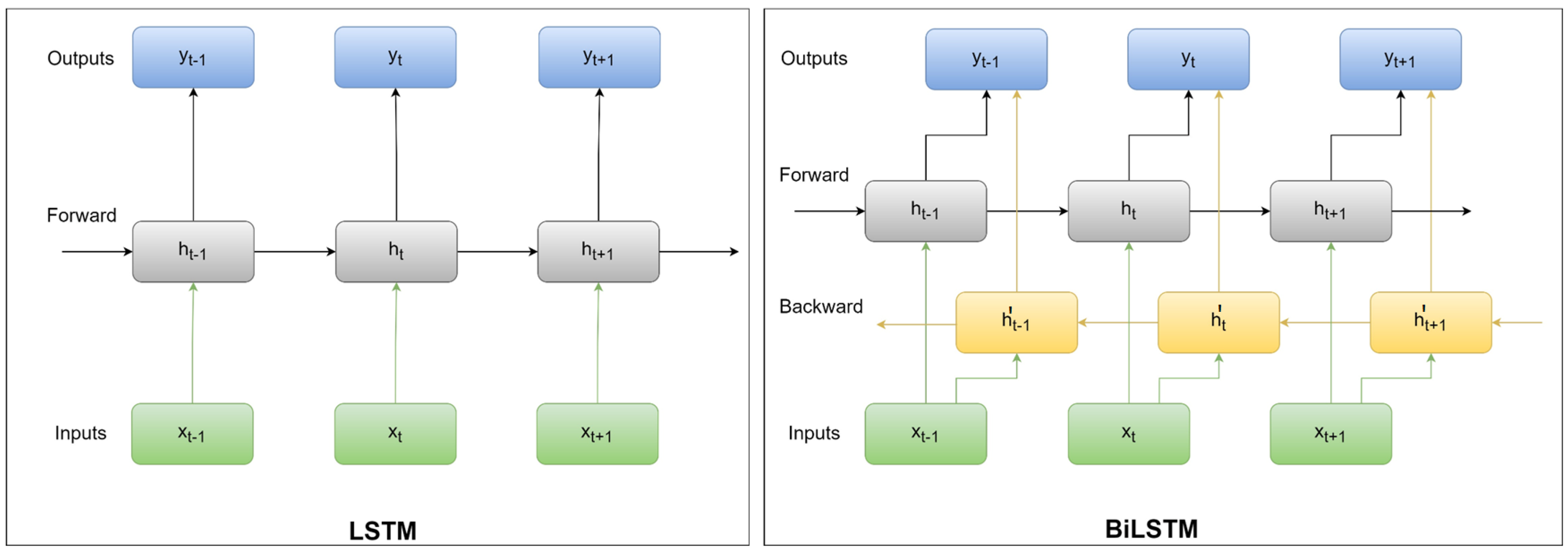
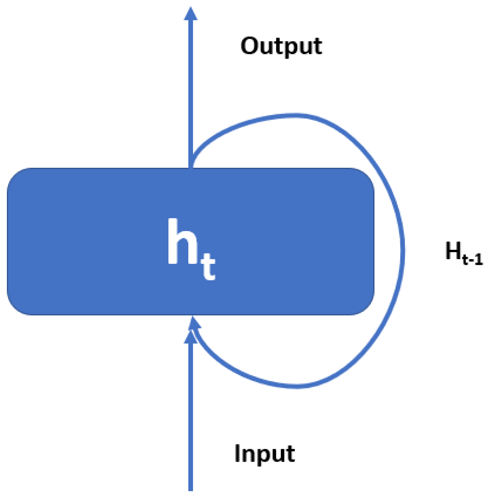
2.2. RNN and BiLSTM
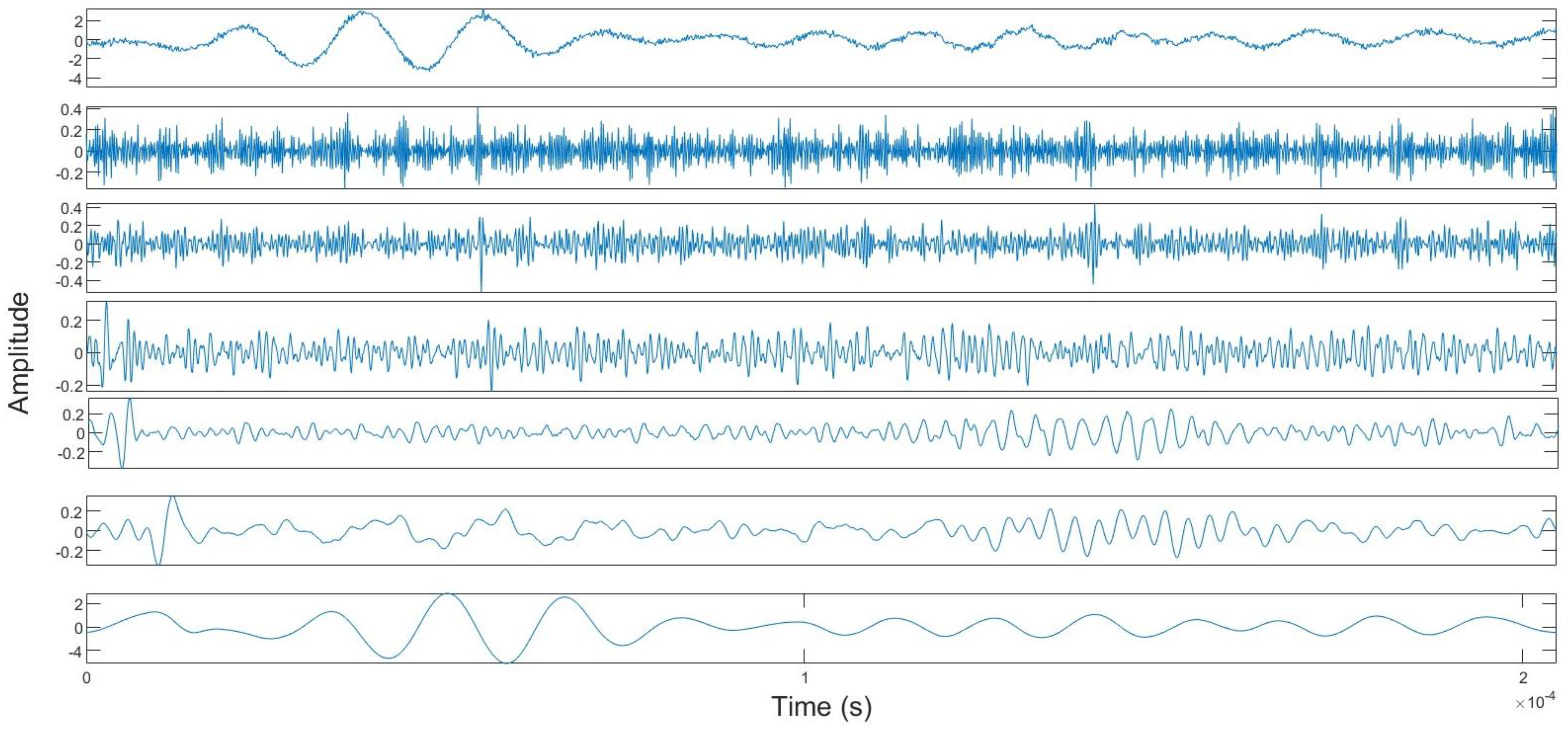
2.3. Maximal Overlap Discrete Wavelet Transform
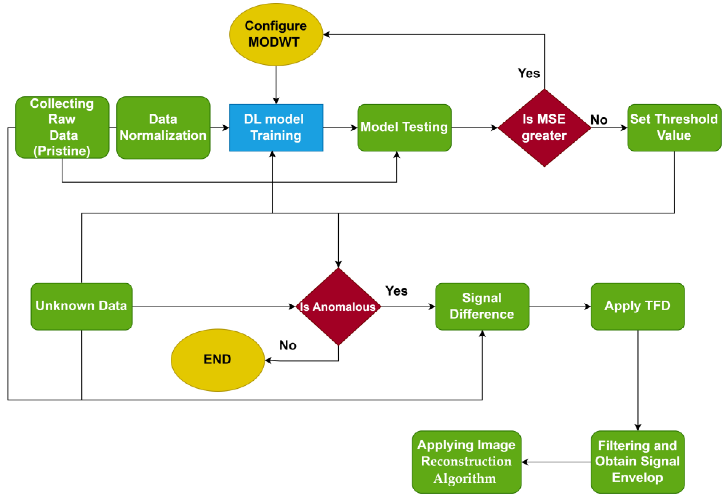
3. Methodology
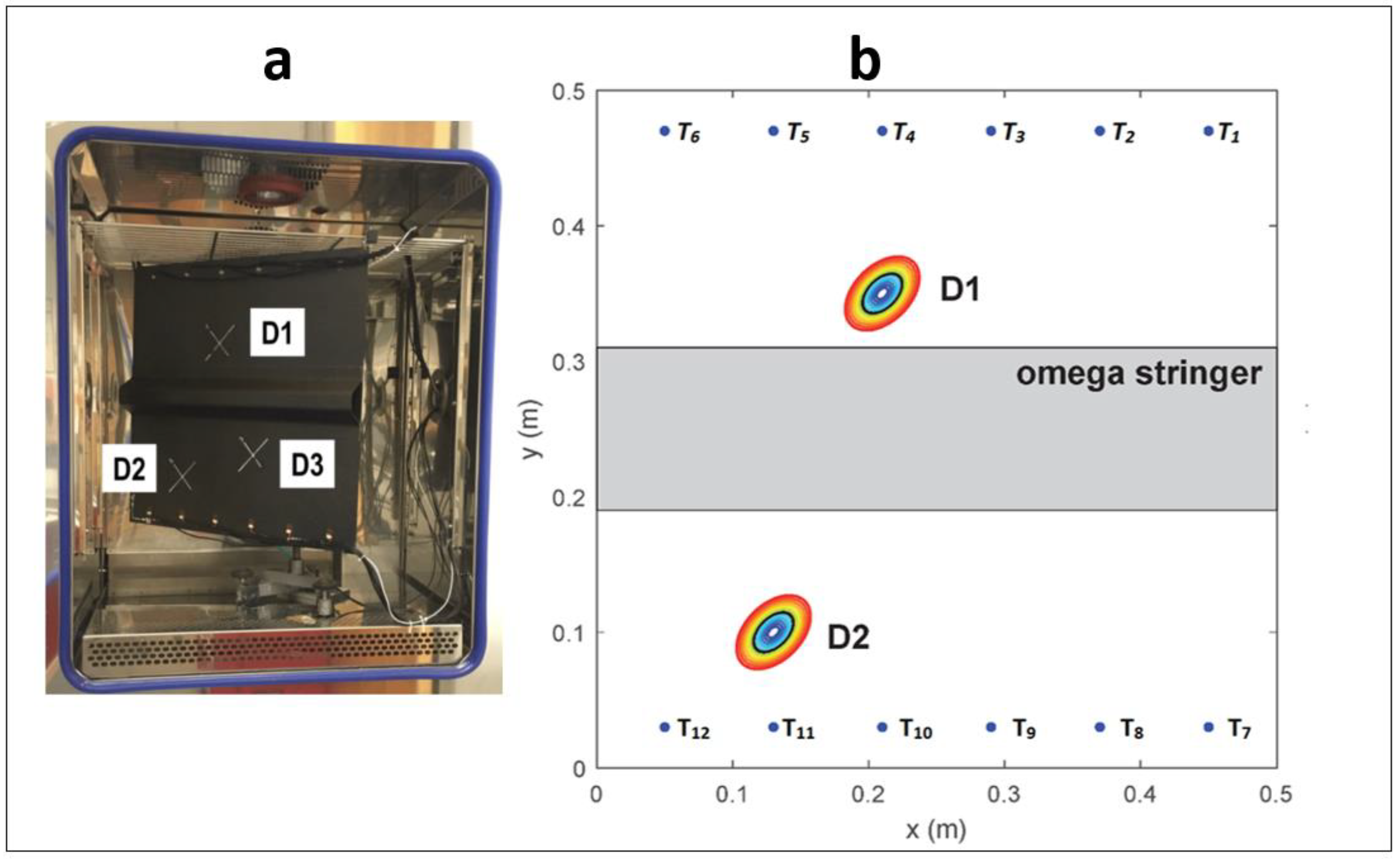
3.1. Experimental Datasets
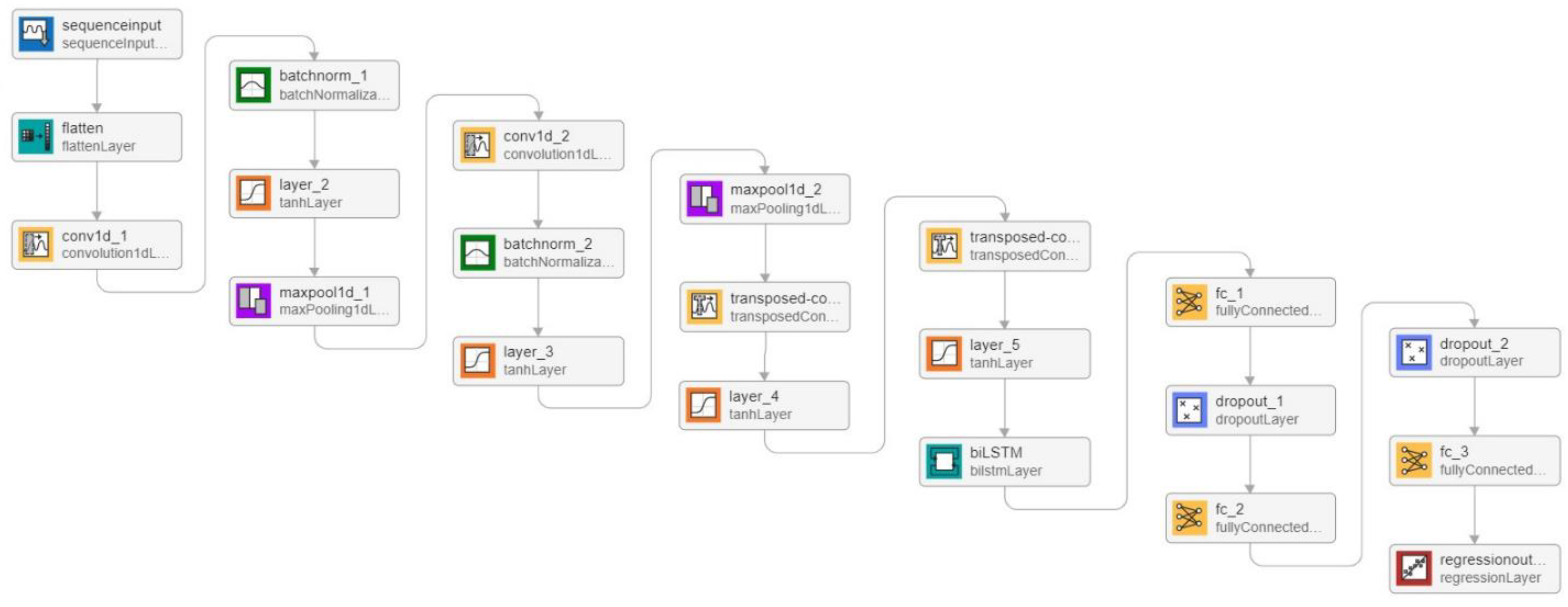
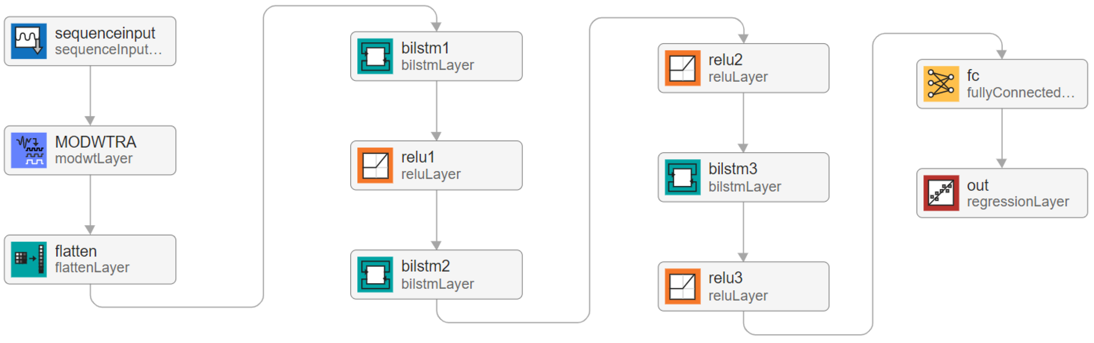
3.2. Model Training
4. Methodology
4.1. Anomaly Detection
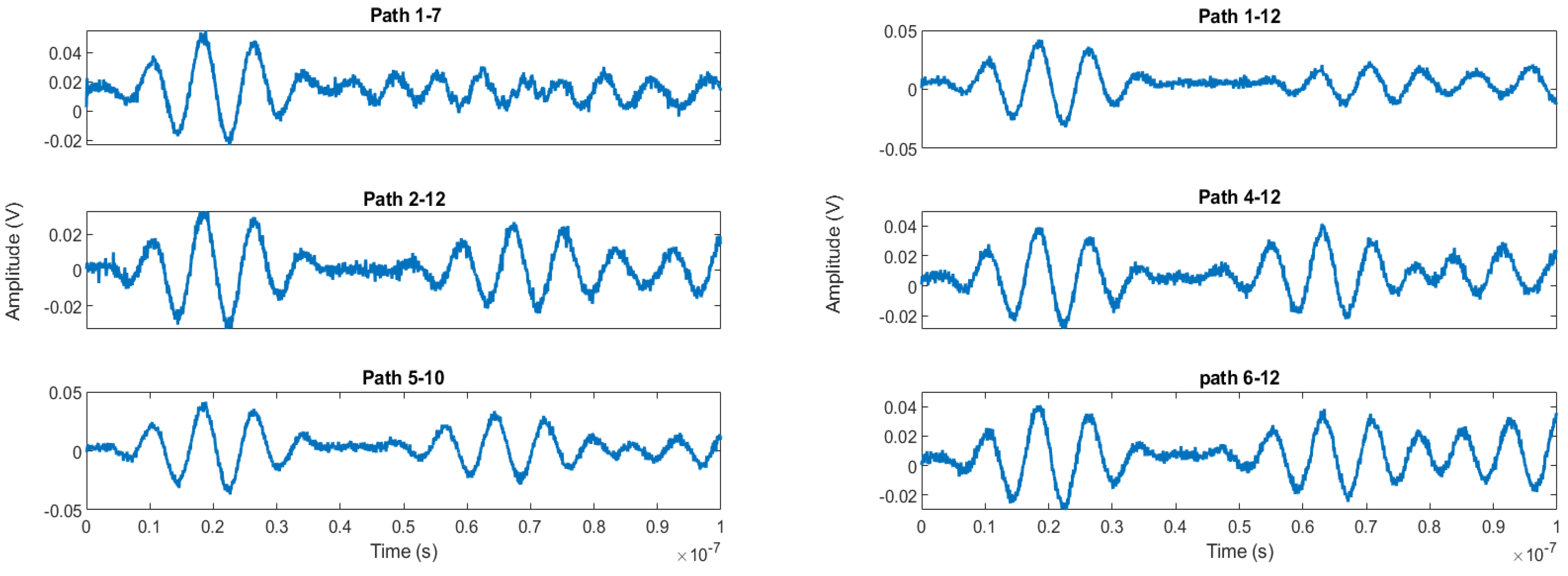
4.2. Damage Localization
5. Conclusions
Author Contributions
Funding
Institutional Review Board Statement
Informed Consent Statement
Data Availability Statement
Conflicts of Interest
References
- Cho, S.; Yun, C.-B.; Lynch, J.P.; Zimmerman, A.T.; Spencer, B.F., Jr.; Nagayama, T. Smart Wireless Sensor Technology for Structural Health Monitoring of Civil Structures. Steel Struct. 2008, 8, 267–275. [Google Scholar]
- Giurgiutiu, V. Structural Health Monitoring with Piezoelectric Wafer Active Sensors: With Piezoelectric Wafer Active Sensors; Elsevier: Amsterdam, The Netherlands, 2007; ISBN 0080556795. [Google Scholar]
- Giurgiutiu, V. Lamb Wave Generation with Piezoelectric Wafer Active Sensors for Structural Health Monitoring. In Proceedings of the Smart Structures and Materials 2003: Smart Structures and Integrated Systems; International Society for Optics and Photonics, San Diego, CA, USA, 2–6 March 2002; Volume 5056, pp. 111–123. [Google Scholar]
- Ye, X.W.; Jin, T.; Yun, C.B. A Review on Deep Learning-Based Structural Health Monitoring of Civil Infrastructures. Smart Struct. Syst. 2019, 24, 567–585. [Google Scholar]
- Alazzawi, O.; Wang, D. Damage Identification Using the PZT Impedance Signals and Residual Learning Algorithm. J. Civ. Struct. Health Monit. 2021, 11, 1225–1238. [Google Scholar] [CrossRef]
- Wang, X.; Mazumder, R.K.; Salarieh, B.; Salman, A.M.; Shafieezadeh, A.; Li, Y. Machine learning for risk and resilience assessment in structural engineering: Progress and future trends. J. Struct. Eng. 2022, 148, 3122003. [Google Scholar]
- Zhang, Z.; Pan, H.; Wang, X.; Lin, Z. Machine Learning-Enriched Lamb Wave Approaches for Automated Damage Detection. Sensors 2020, 20, 1790. [Google Scholar] [CrossRef]
- Zhang, Z.; Sun, C. Structural Damage Identification via Physics-Guided Machine Learning: A Methodology Integrating Pattern Recognition with Finite Element Model Updating. Struct. Health Monit. 2021, 20, 1675–1688. [Google Scholar] [CrossRef]
- Rai, A.; Mitra, M. Lamb Wave Based Damage Detection in Metallic Plates Using Multi-Headed 1-Dimensional Convolutional Neural Network. Smart Mater. Struct. 2021, 30, 35010. [Google Scholar] [CrossRef]
- Wang, X.; Zhang, X.; Shahzad, M.M. A Novel Structural Damage Identification Scheme Based on Deep Learning Framework. Structures 2021, 29, 1537–1549. [Google Scholar] [CrossRef]
- Xu, L.; Yuan, S.; Chen, J.; Ren, Y. Guided Wave-Convolutional Neural Network Based Fatigue Crack Diagnosis of Aircraft Structures. Sensors 2019, 19, 3567. [Google Scholar] [CrossRef]
- Li, S.; Zuo, X.; Li, Z.; Wang, H. Applying Deep Learning to Continuous Bridge Deflection Detected by Fiber Optic Gyroscope for Damage Detection. Sensors 2020, 20, 911. [Google Scholar] [CrossRef]
- Hung, D.V.; Hung, H.M.; Anh, P.H.; Thang, N.T. Structural Damage Detection Using Hybrid Deep Learning Algorithm. J. Sci. Technol. Civ. Eng. (STCE)-NUCE 2020, 14, 53–64. [Google Scholar] [CrossRef]
- Momeni, H.; Ebrahimkhanlou, A. High-Dimensional Data Analytics in Structural Health Monitoring and Non-Destructive Evaluation: A Review Paper. Smart Mater. Struct. 2022, 31, 043001. [Google Scholar]
- Gao, Y.; Liu, X.; Xiang, J. Fault Detection in Gears Using Fault Samples Enlarged by a Combination of Numerical Simulation and a Generative Adversarial Network. IEEE/ASME Trans. Mechatron. 2021, 27, 3798–3805. [Google Scholar] [CrossRef]
- Taylor, L.; Nitschke, G. Improving Deep Learning with Generic Data Augmentation. In Proceedings of the 2018 IEEE Symposium Series on Computational Intelligence, Bangalore, India, 18–21 November 2018. [Google Scholar]
- Oh, C.; Han, S.; Jeong, J. Time-Series Data Augmentation Based on Interpolation. Procedia Comput. Sci. 2020, 175, 64–71. [Google Scholar] [CrossRef]
- Cui, X.; Goel, V.; Kingsbury, B. Data Augmentation for Deep Neural Network Acoustic Modeling. IEEE/ACM Trans. Audio Speech Lang. Process. 2015, 23, 1469–1477. [Google Scholar]
- Li, W.; Chen, C.; Zhang, M.; Li, H.; Du, Q. Data Augmentation for Hyperspectral Image Classification with Deep CNN. IEEE Geosci. Remote Sens. Lett. 2019, 16, 593–597. [Google Scholar] [CrossRef]
- Reconstruct Inputs to Detect Anomalies, Remove Noise, and Generate Images and Text. Available online: https://www.mathworks.com/discovery/autoencoder.html (accessed on 11 June 2023).
- Torabi, H.; Mirtaheri, S.L.; Greco, S. Practical Autoencoder Based Anomaly Detection by Using Vector Reconstruction Error. Cybersecurity 2023, 6, 1. [Google Scholar] [CrossRef]
- Recurrent Neural Network (RNN). Available online: https://www.mathworks.com/discovery/rnn.html (accessed on 11 June 2023).
- Said Elsayed, M.; Le-Khac, N.-A.; Dev, S.; Jurcut, A.D. Network Anomaly Detection Using LSTM Based Autoencoder. In Proceedings of the 16th ACM Symposium on QoS and Security for Wireless and Mobile Networks, Alicante, Spain, 16–20 November 2020; pp. 37–45. [Google Scholar]
- Lu, Y.; Tang, L.; Chen, C.; Zhou, L.; Liu, Z.; Liu, Y.; Jiang, Z.; Yang, B. Reconstruction of Structural Long-Term Acceleration Response Based on BiLSTM Networks. Eng. Struct. 2023, 285, 116000. [Google Scholar] [CrossRef]
- Li, S.; Li, W.; Cook, C.; Zhu, C.; Gao, Y. Independently Recurrent Neural Network (Indrnn): Building a Longer and Deeper Rnn. In Proceedings of the IEEE Conference on Computer Vision and Pattern Recognition, Salt Lake City, UT, USA, 18–23 June 2018; pp. 5457–5466. [Google Scholar]
- Maximal Overlap Discrete Wavelet Transform. Available online: https://www.mathworks.com/help/wavelet/ref/modwt.html (accessed on 11 June 2023).
- Xiao, F.; Lu, T.; Wu, M.; Ai, Q. Maximal Overlap Discrete Wavelet Transform and Deep Learning for Robust Denoising and Detection of Power Quality Disturbance. IET Gener. Transm. Distrib. 2020, 14, 140–147. [Google Scholar] [CrossRef]
- Moll, J.; Kexel, C.; Kathol, J.; Fritzen, C.-P.; Moix-Bonet, M.; Willberg, C.; Rennoch, M.; Koerdt, M.; Herrmann, A. Guided Waves for Damage Detection in Complex Composite Structures: The Influence of Omega Stringer and Different Reference Damage Size. Appl. Sci. 2020, 10, 3068. [Google Scholar]
- Rizvi, S.H.; Abbas, M. Lamb Wave Damage Severity Estimation Using Ensemble-Based Machine Learning Method with Separate Model Network. Smart Mater. Struct. 2021, 30, 115016. [Google Scholar] [CrossRef]


| Transducer/Sensor ID | Coordinates |
|---|---|
| 1 | (450, 470) |
| 2 | (370, 470) |
| 3 | (290, 470) |
| 4 | (210, 470) |
| 5 | (130, 470) |
| 6 | (50, 470) |
| 7 | (450, 30) |
| 8 | (370, 30) |
| 9 | (290, 30) |
| 10 | (210, 30) |
| 11 | (130, 30) |
| 12 | (50, 30) |
| Layers | Learnable Properties | Number of Learnable | |
|---|---|---|---|
| 1 | Sequence input | ||
| 2 | MODWT | Weights 3 × 30 | 60 |
| 3 | Flatten | ||
| 4 | biLSTM 1 (32 hidden units) | Input weights = 128 × 5 Recurrent weights = 128 × 16 Bias = 128 × 1 | 2816 |
| 5 | Relu 1 | ||
| 6 | biLSTM 2 (64 hidden units) | Input weights = 256 × 32 Recurrent weights = 256 × 32 Bias = 256 × 1 | 16,640 |
| 7 | Relu 2 | ||
| 8 | biLSTM 3 (32 hidden units) | Input weights = 128 × 64 Recurrent weights = 128 × 16 Bias = 128 × 1 | 10,368 |
| 9 | Relu 3 | ||
| 10 | Fully Connected | Weights = 1 × 32 Bias = 1 × 1 | 33 |
| 11 | Regression Output | ||
| Total | 29,900 | ||
| Deep-Learning Models | Accuracy | RMSE | MAE |
|---|---|---|---|
| 1D CNN | 81.44% | 0.2347 | 0.1856 |
| Bi-LSTM | 84.75% | 0.1950 | 0.1522 |
| MODWT + Bi-LSTM | 86.1% | 0.1830 | 0.1439 |
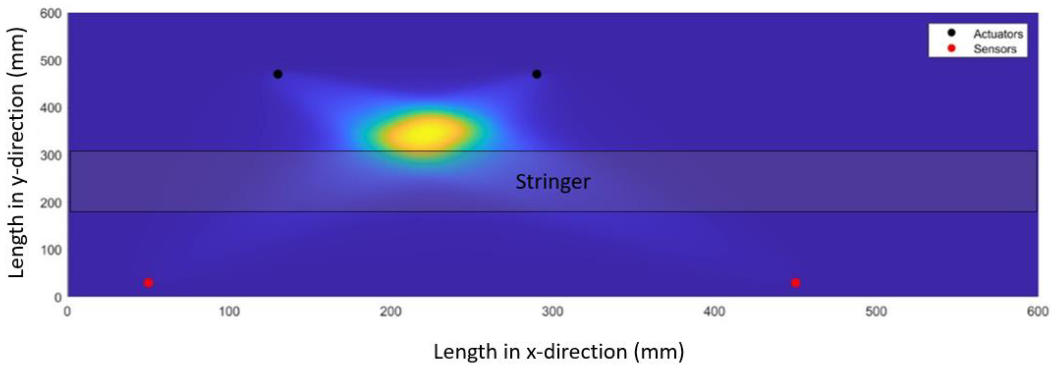
| Damage ID | x-Coordinates (mm) | y-Coordinates (mm) |
|---|---|---|
| D1 | 210 | 350 |
| D2 | 130 | 100 |
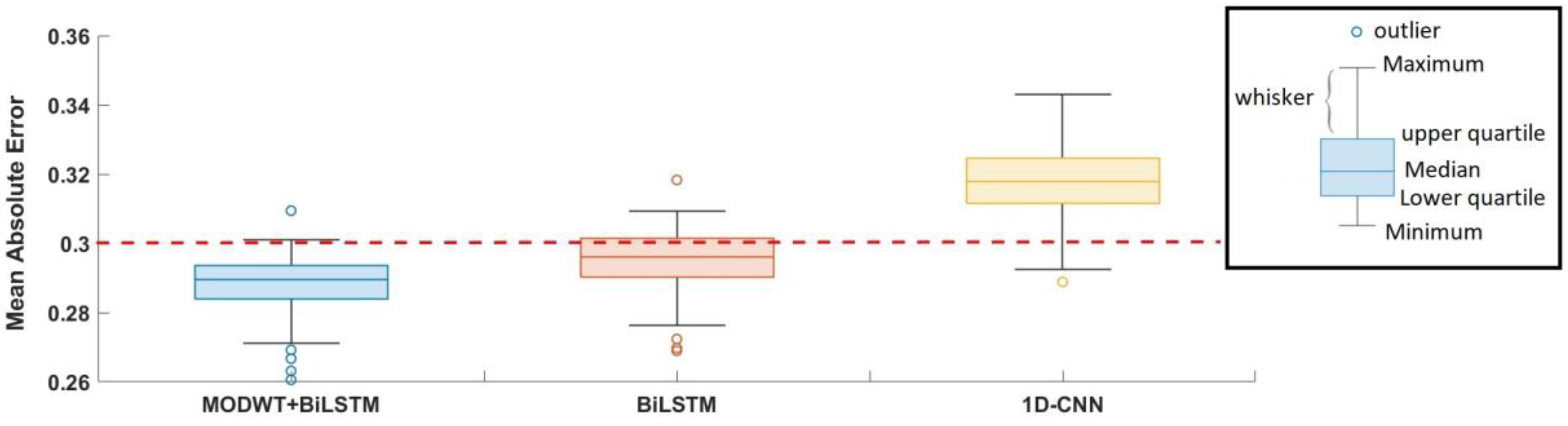
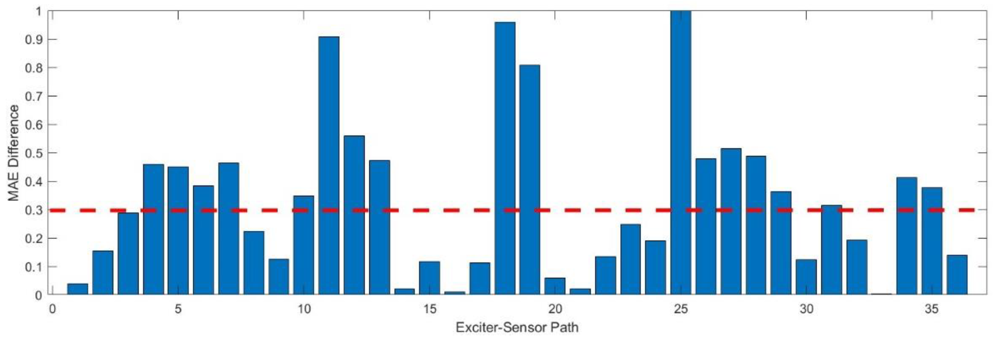
| MODWT + RNN | RNN | 1D-CNN |
|---|---|---|
| 0.300 | 0.315 | 0.350 |
| Deep Learning Models | True Anomaly Detection | False/Missed Detection | Accuracy |
|---|---|---|---|
| MODWT + BiLSTM | 385 | 51 | 88.3% |
| BiLSTM | 375 | 61 | 86.0% |
| 1D-CNN | 351 | 85 | 80.5% |
| Damage ID | Average MAE Difference |
|---|---|
| D1 | 0.37 |
| D2 | 0.48 |
Disclaimer/Publisher’s Note: The statements, opinions and data contained in all publications are solely those of the individual author(s) and contributor(s) and not of MDPI and/or the editor(s). MDPI and/or the editor(s) disclaim responsibility for any injury to people or property resulting from any ideas, methods, instructions or products referred to in the content. |
© 2024 by the authors. Licensee MDPI, Basel, Switzerland. This article is an open access article distributed under the terms and conditions of the Creative Commons Attribution (CC BY) license (https://creativecommons.org/licenses/by/4.0/).
Share and Cite
Rizvi, S.H.M.; Abbas, M.; Zaidi, S.S.H.; Tayyab, M.; Malik, A. LSTM-Based Autoencoder with Maximal Overlap Discrete Wavelet Transforms Using Lamb Wave for Anomaly Detection in Composites. Appl. Sci. 2024, 14, 2925. https://doi.org/10.3390/app14072925
Rizvi SHM, Abbas M, Zaidi SSH, Tayyab M, Malik A. LSTM-Based Autoencoder with Maximal Overlap Discrete Wavelet Transforms Using Lamb Wave for Anomaly Detection in Composites. Applied Sciences. 2024; 14(7):2925. https://doi.org/10.3390/app14072925
Chicago/Turabian StyleRizvi, Syed Haider Mehdi, Muntazir Abbas, Syed Sajjad Haider Zaidi, Muhammad Tayyab, and Adil Malik. 2024. "LSTM-Based Autoencoder with Maximal Overlap Discrete Wavelet Transforms Using Lamb Wave for Anomaly Detection in Composites" Applied Sciences 14, no. 7: 2925. https://doi.org/10.3390/app14072925
APA StyleRizvi, S. H. M., Abbas, M., Zaidi, S. S. H., Tayyab, M., & Malik, A. (2024). LSTM-Based Autoencoder with Maximal Overlap Discrete Wavelet Transforms Using Lamb Wave for Anomaly Detection in Composites. Applied Sciences, 14(7), 2925. https://doi.org/10.3390/app14072925