Comparative Analysis of Local Differential Privacy Schemes in Healthcare Datasets

Abstract

In the rapidly evolving landscape of healthcare technology, the critical need for robust privacy safeguards is undeniable. Local Differential Privacy (LDP) offers a potential solution to address privacy concerns in data-rich industries. However, challenges such as the curse of dimensionality arise when dealing with multidimensional data. This is particularly pronounced in k-way joint probability estimation, where higher values of k lead to decreased accuracy. To overcome these challenges, we propose the integration of Bayesian Ridge Regression (BRR), known for its effectiveness in handling multicollinearity. Our approach demonstrates robustness, manifesting a noteworthy reduction in average variant distance when compared to baseline algorithms such as LOPUB and LOCOP. Additionally, we leverage the R-squared metric to highlight BRR’s advantages, illustrating its performance relative to LASSO, as LOPUB and LOCOP are based on it. This paper addresses a relevant concern related to datasets exhibiting high correlation between attributes, potentially allowing the extraction of information from one attribute to another. We convincingly show the superior performance of BRR over LOPUB and LOCOP across 15 datasets with varying average correlation attributes. Healthcare takes center stage in this collection of datasets. Moreover, the datasets explore diverse fields such as finance, travel, and social science. In summary, our proposed approach consistently outperforms the LOPUB and LOCOP algorithms, particularly when operating under smaller privacy budgets and with datasets characterized by lower average correlation attributes. This signifies the efficacy of Bayesian Ridge Regression in enhancing privacy safeguards in healthcare technology.

1. Introduction

In the ever-evolving realm of healthcare technology, the implementation of robust privacy safeguards has become indispensable. A pivotal approach in this regard is the utilization of local differential privacy, a technique devised to safeguard individual-level data while simultaneously facilitating the extraction of valuable insights from aggregated datasets. As the healthcare industry increasingly embraces digital solutions and data-driven decision-making, the necessity to strike a balance between innovation and the protection of sensitive patient information has become more pressing than ever.

Nowadays, our data are multidimensional, making it possible to extract vast amounts of information. For instance, a healthcare institution with a dataset tracking patient activities can glean valuable insights. A patient’s interactions within a hospital environment, treated as high-dimensional data, can be analyzed to uncover patterns such as patient admission and discharge times, the duration of medical procedures, staff interactions, and preferred modes of transportation within the hospital premises, among other relevant metrics.

In recent years, safeguarding personal data privacy has gained heightened significance, driven by the expanding array of industries, not limited to healthcare, that actively collect and store our information. A significant privacy concern revolves around data publishing, and one approach to tackle this issue is through Central Differential Privacy (CDP) [1]. This method facilitates the release of sensitive data, permitting statistical analysis while preserving individual privacy. However, it is important to note that in CDP, users are required to share their original information with a central server. In contrast, LDP aims to address this limitation. Unlike CDP, users in LDP do not need to place trust in the communication channel or central server. Instead, they encode their data and introduce random noise before transmitting it to the central server. This process effectively protects users’ privacy while still enabling the central server to compute the distribution of user statistics.

Arcolezi et al. [2] and Yang et al. [3] provide overviews of LDP technology, summarizing and analyzing state-of-the-art research in the field. Yang [3] provides an overview of existing works that serves as a foundational resource for exploring emerging challenges in the future. These challenges include the relaxation of LDP, privacy amplification, and the development of solutions tailored for small populations. Meanwhile, Arcolezi [2] investigates the impact of collecting multiple sensitive attributes under LDP on fairness. They experiment with several LDP approaches, including Generalized Randomized Response (GRR), Binary Local Hashing (BLH), Optimal Local Hashing (OLH), RAPPOR, Optimal Unary Encoding (OUE), Subset Selection (SS), and Thresholding with Histogram Encoding (THE) to train Machine Learning (ML) models. The models are then evaluated using several metrics, including the F1-score, area under the receiver operating characteristic curve (AUC), Disparate Impact (DI), Statistical Parity Difference (SPD), Equal Opportunity Difference (EOD), and Overall Accuracy Difference (OAD). The differences between Arcolezi [2] and our work are presented in Table 1.

RAPPOR [4] is one of the most well-known LDP approaches; it was developed by Google as an extension of Google Chrome, which collects process names and homepages from users using an LDP algorithm. Furthermore, Apple has incorporated an LDP application into their devices [5], intended for identifying popular emojis and detecting high energy and memory usage in their devices. These examples represent just a few instances of the diverse applications of LDP in practice. Nevertheless, the application of LDP schemes faces challenges when dealing with multi-dimensional data, primarily stemming from dimensionality issues like the curse of dimensionality. This concept asserts that as the data’s dimensionality grows, introducing sufficient noise to protect privacy becomes increasingly challenging without excessively distorting the data. For instance, consider a dataset with 10 features. Achieving local differential privacy would require perturbing each feature with a specific amount of random noise. However, if we increase the number of features to 100, the noise to maintain the same level of privacy also increases.

To tackle these challenges, several studies have been conducted. Ren et al. proposed LOPUB [6], a privacy-preserving technique where users first encode their data using Bloom filters and then perturb the encoded data using the randomized response (RR) algorithm [7]. Finally, the perturbed-encoded data are sent to a central server, which estimates the multi-dimensional joint probability distribution by applying the LASSO [8] and expectation-maximization (EM) algorithms [9]. This method was tested on open datasets and demonstrated good performance for high-dimensional data with low multi-dimensional joint probability distributions. Meanwhile, LOCOP [10] represents a novel approach for preserving privacy in high-dimensional data through synthesis. A univariate marginal distribution is computed using LASSO regression from the perturbed-encoded data, and a multivariate Gaussian copula is used to model the attribute dependence. This method aims to provide a privacy-preserving solution for sharing high-dimensional data with a central server.

Regrettably, approaches like LOPUB encounter diminished data utility as k-way increases, where k is the dimensionality of joint probability distribution estimation. For certain datasets, the error between $k=2$ and $k=3$ evaluations can be two or three times higher, contingent upon the cardinality of the attributes. Another crucial factor to take into account is the number of elements in each attribute domain. Consequently, these methods only offer a partial resolution to the challenge of handling extensive datasets with numerous attributes and high cardinality. Unfortunately, both LOPUB and LOCOP rely on LASSO regression, initially introduced to enhance prediction accuracy in regression models. However, the LASSO regularization technique, employed in linear regression, grapples with high cardinality—a prevalent issue for large datasets. The encoding and perturbation method introduced by [6] has also been utilized and built upon in subsequent works such as Wang [10] and Jiang [11].

We propose the application of the Bayesian Ridge Regression (BRR) of Yang and Emura [3] on the central server to address the challenge of evaluating highly correlated attributes. The differences between our approach  [6], and [10] are outlined in Table 1.

This work is supported by the research of Wieringen et al. [12], Sambasivan et al. [13], and Assat et al. [14]. Wieringen’s investigation focused on computing the posterior probability from the prior probability, providing several benefits, including the construction of robust prior distributions. Additionally, Sambasivan [13] applied a Bayesian approach in sparse modeling and machine learning. Assat et al. [14] demonstrated the effectiveness of this approach in constructing reliable prior probability distributions. This collective evidence underscores the value of investigating BRR, suggesting practical applications across diverse fields. Our previous work (a preliminary version of this work was published in [15]) laid the groundwork for integrating BRR within the LDP mechanism, and the extended version of this work delves deeply into exploring attribute correlations using the average absolute Pearson correlation. This comprehensive expansion goes beyond the mere application of BRR; it involves nuanced analyses of privacy guarantees and complexity trade-offs, employing various metrics such as R-squared. Additionally, it includes a comparison between regression techniques applied to estimate joint probability distributions in LDP. This study also encompasses several experiments on datasets with different characteristics, including variations in size, attribute composition, and correlation from various industries. Among these datasets are well-known sets commonly used to evaluate LDP or CDP approaches.

Healthcare takes center stage in this collection of datasets. This evaluation is made because datasets in the healthcare domain often exhibit high correlations among attributes. For instance, the risk of developing various diseases tends to increase with age, encompassing conditions such as heart disease, stroke, cancer, and Alzheimer’s disease. This phenomenon arises from multiple factors, including changes in cell function, the accrual of damage over time, and the decline of the immune system. Certain diseases also exhibit age-related prevalence, with childhood cancer being more common in children and prostate cancer being more prevalent in older men.

Another solution to apply LDP into medical datasets was proposed by Sung et al. [16]. They normalized all data to a range between −1 and 1, and they applied the bounded Laplacian method to prevent the generation of out-of-bound values following the application of the differential privacy algorithm. To preserve the cardinality of categorical variables, postprocessing via discretization was conducted. The efficacy of the algorithm was assessed using both synthetic and real-world data sourced from the eICU Collaborative Research Database. Evaluation involved comparing the original and perturbed data using misclassification rates for categorical data and the mean squared error for continuous data on ML models. Furthermore, the researchers compared the performance of classification models predicting in-hospital mortality using real-world data. The differences between this work and ours is presented in Table 1.

Table 1. Differences between Sung [16], Arcolezi [2], LOPUB [6], LOCOP [10], and this paper. The datasets pertaining to the healthcare industry are underlined.

	Datasets	Perturbation	Estimation	Evaluation
Sung [16]	Synthetic eICU	Normalize Bounded Laplacian Discretization	NA	(ML Models) misclassification rates mean squared error
Arcolezi [2]	Adults ACSCoverage LSAC	GRR BLH OLH RAPPOR OUE SS THE	NA	(ML Models) f1-score AUC DI SPD EOD OAD
LOPUB [6]	Nursery Lung Cancer  Stroke	Bloom Filter Randomize Respose	LASSO with EM
LOCOP [10]	NHANES Bank National Massachusets Texas		LASSO with Gaussian Copula	Joint probability distribution
Ours	MS FIMU Adults Hypertension Skin Cancer Diabetes US CENSUS Cirrhosis		BRR [17]	AVD

Table 1. Differences between Sung [16], Arcolezi [2], LOPUB [6], LOCOP [10], and this paper. The datasets pertaining to the healthcare industry are underlined.

	Datasets	Perturbation	Estimation	Evaluation
Sung [16]	Synthetic eICU	Normalize Bounded Laplacian Discretization	NA	(ML Models) misclassification rates mean squared error
Arcolezi [2]	Adults ACSCoverage LSAC	GRR BLH OLH RAPPOR OUE SS THE	NA	(ML Models) f1-score AUC DI SPD EOD OAD
LOPUB [6]	Nursery Lung Cancer  Stroke	Bloom Filter Randomize Respose	LASSO with EM
LOCOP [10]	NHANES Bank National Massachusets Texas		LASSO with Gaussian Copula	Joint probability distribution
Ours	MS FIMU Adults Hypertension Skin Cancer Diabetes US CENSUS Cirrhosis		BRR [17]	AVD

We assess the performance of LOPUB [6], LOCOP [10], and BRR using three metrics: average variant distance (AVD), R-squared, and the average absolute Pearson correlation coefficient (AAR). AVD is employed to quantify the difference between the probabilities of two joint probability distributions—the original and those computed by the LDP approaches. Subsequently, we propose using R-squared, a metric that gauges the performance of LASSO and Bayesian Ridge Regression algorithms applied to LDP approaches. Finally, we evaluate how the performance of LDP approaches is affected by the correlation between elements in a dataset using AAR.

With a privacy budget set to $ϵ=0.1$ per attribute and $k=5$, after conducting one hundred experiments, our work achieves a 57% reduction in the average variant distance compared to that of LOPUB. The contributions of this paper are summarized as follows:

• We propose a new LDP schema using BRR for joint probability estimation and the baseline algorithm LOPUB [6].
• We propose two metrics, R-squared and AAR, for evaluation of the performance.
• We show in this document the experimental results using six open datasets that demonstrates the superiority of estimation accuracy and the robustness across diverse characteristics including numbers of users, attributes, and AARs.

The subsequent sections of the paper are organized as follows: Section 2 provides the preliminaries, while Section 3 details our proposed approach. The paper concludes with the sections Experiments and Conclusions.

2. Preliminaries

2.1. LDP Overview and the Curse of High Dimensionality

The Local Differential Privacy (LDP) model comprises two entities: users and a central server, with the objective of enabling users to share information while safeguarding their privacy. The shared information serves various purposes, including computing statistics about the dataset. LDP has proven effective in sharing and recovering the original distribution of a dataset while preserving user privacy. Numerous LDP approaches in the literature employ diverse methods to protect user information [1,4,18].

As a general example, we can think of a dataset where the attributes exhibit the following cardinalities ${\mathsf{\Omega }}_{gender}$ = {male, female}, ${\mathsf{\Omega }}_{country}=\{USA,CAN,CHN,JAP,MEX\}$, and ${\mathsf{\Omega }}_{marital}$ = {married, widowed, separated, divorced, single}. The objective of LDP is for users to transmit their information to the central server while preserving anonymity. Subsequently, the central server can use the information provided by the users to compute the original distribution of this dataset.

In this example, if the central server tries to recover the distribution of one attribute, it will face the original cardinalities $|{\mathsf{\Omega }}_{gender}|=2$, $|{\mathsf{\Omega }}_{marital}|=5$, and $|{\mathsf{\Omega }}_{country}|=5$, where the average of these cardinalities is computed as

$$\begin{array}{c}\overline{{\omega }_k}=\frac{{\sum }_k\left|{\mathsf{\Omega }}_{\left(\genfrac{}{}{0pt}{}{gender,marital,country}{k}\right)}\right|}{\left(\genfrac{}{}{0pt}{}{gender,marital,country}{k}\right)}.\end{array}$$

(1)

Here, $|{\mathsf{\Omega }}_{\left(\genfrac{}{}{0pt}{}{gender,marital,country}{k}\right)}|$ denotes the cardinality of the unique combinations of the attributes for gender, marital status, and country, while $\left(\genfrac{}{}{0pt}{}{gender,marital,country}{k}\right)$ represents the count of unique combinations for a given value of k. The average of these cardinalities is computed using Equation (1). Substituting ($k=1$), the result is $\overline{{\omega }_1}=\frac{{\sum }_1\left|{\mathsf{\Omega }}_{\left(\genfrac{}{}{0pt}{}{gender,marital,country}{1}\right)}\right|}{\left(\genfrac{}{}{0pt}{}{gender,marital,country}{1}\right)}=\frac{2+5+5}{3}=4$, and the cardinality has risen; for two attributes ($k=2$), the average is $\overline{{\omega }_2}=15$. Finally, the cardinality of three attributes ($k=3$) is $\overline{{\omega }_3}=50$. The complexity of the cardinality increases as the number of attributes grows. For instance, consider a real-world dataset with tens of attributes. We can see the challenge when the central server tries to recover k attributes, as the average cardinality size increases with the data dimensionality.

2.2. Correlation between Variables in Healthcare Datasets

In the realm of healthcare datasets, the question of whether there is a correlation between variables becomes pivotal, especially considering the sensitivity of health-related information. Here, there are some examples of some kinds of datasets that can have correlations between their attributes:

• Age and Disease Risk:

  −

  The risk of developing many diseases increases with age.

  −

  Certain diseases are more likely to occur in specific age groups.

• Body Mass Index (BMI) and Diabetes:

  −

  People with a higher BMI are more likely to develop type 2 diabetes.

  −

  Excess body weight can lead to insulin resistance, increasing the risk of diabetes.

• Blood Pressure and Cardiovascular Diseases:

  −

  High blood pressure is a major risk factor for cardiovascular diseases.

  −

  The risk of developing cardiovascular diseases increases with blood pressure.

• Cholesterol Levels and Atherosclerosis:

  −

  High levels of LDL (bad) cholesterol can lead to atherosclerosis.

  −

  The risk of developing atherosclerosis increases with LDL cholesterol levels.

• Exercise Habits and Overall Health:

  −

  Regular exercise has many health benefits, including a reduced risk of various conditions.

  −

  Exercise also helps to improve mental health and overall mood.

• Smoking and Respiratory Diseases:

  −

  Smoking is a leading cause of preventable death.

  −

  Smoking is a major risk factor for respiratory diseases.

R-Squared, $R^2$

Despite the ubiquity of regression analysis in scientific disciplines, a unified standard for its evaluation remains elusive. Chicco et al. [19] perform a critical review, examining several commonly employed metrics and ultimately advocate for R-squared as the most informative and transparent measure in many cases. While metrics such as mean absolute percentage error (MAPE), mean absolute error (MAE), mean square error (MSE), and its rooted variant (RMSE) are frequently used, they often obscure crucial details about a regression model’s performance. For example, a seemingly acceptable MAPE value can conceal significant outliers or systematic biases. In contrast, Chicco et al. [19] show that R-squared offers valuable clarity: high values denote accurate predictions across diverse data points, while negative values unambiguously signal a poorly fitting model. This inherent informativeness makes R-squared a compelling choice for evaluating regression analyses in various scientific contexts. R-squared is computed as

$$\begin{array}{c}{R}^2=1-\frac{MSE}{MST},\end{array}$$

where $MSE$ is ${\sum }_{i=1}^z{(X_i-C_i)}^2$ and the mean total sum of squares ($MST$) is ${\sum }_{i=1}^z{(Y_i-\overline{Y})}^2$. In the previous formulas, $X_i$ is the predicted ith value, the $C_i$ element is the actual ith value, and z is the length of the vector. In our experiments, $X_i$ and $C_i$ are the joint probability distributions for real and computed data on k-way. R-squared can take values in the range $(-\infty ,1]$ according to the mutual relation between the ground truth and the prediction model. Hereafter, we show a brief overview of the principal cases.

• $R^2\ge 0$: With linear regression with no constraints, $R^2$ is non-negative.
• $R^2=0$: The fitted line (or hyperplane) is horizontal. With two numerical variables, this is the case if the variables are independent, that is, are uncorrelated.
• $R^2\le 0$: This case is only possible with linear regression when either the intercept or the slope are constrained so that the “best-fit” line (given the constraint) fits worse than a horizontal line, for instance, if the regression line (hyperplane) does not follow the data.

2.3. Generalizing the Problem

Before describing our approach, we introduce preliminary concepts. In LDP approaches, users want to not only share their information with a central server but also maintain their privacy. Thus, users encode and perturb their data before sending it to the central server, and in doing this, they preserve their anonymity. In this work, we follow the user steps proposed by LOPUB [6], where we generalize the LDP problem; there are N users, and $U=\{u^1,u^2,u^3,\dots ,u^N\}$ is a set of users. All users have an equal number of attributes, denoted as d. Each attribute has a specific domain, represented by ${\mathsf{\Omega }}_i=\{{\omega }_i^1,\dots ,{\omega }_i^{\left|{\mathsf{\Omega }}_i\right|}\}$, where i ranges from 1 to d.

2.4. Local Differential Privacy

Local Differential Privacy (LDP) [20] offers a stringent privacy guarantee, wherein users place their trust solely in themselves and not in any central authority.

Definition 1 

(Local Differential Privacy). An algorithm ξ satisfies ϵ-local differential privacy for any user if for any two data records u and w and for any output $\tilde{u}$ within the range of outputs of algorithm $\xi (\tilde{u}\subset Range\left(\xi \right))$, Equation (2) holds:

$$\begin{array}{c}Pr[\xi \left(u\right)\in \tilde{u}]\le e^{ϵ}Pr[\xi \left(w\right)\in \tilde{u}].\end{array}$$

(2)

In Equation (2), ϵ is the privacy budget, a smaller ϵ implies stronger privacy protection, while a larger value indicates the opposite.

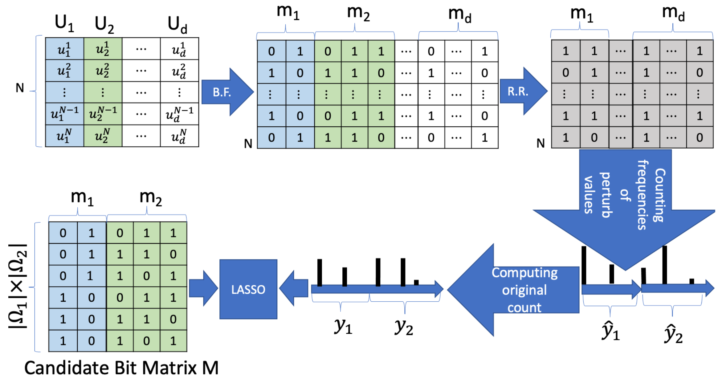
2.5. LOPUB Scheme

The algorithm introduced by Ren [6] for encoding and perturbing user data has been implemented in this study.

Table 2. Notations.

Notation	Description
k	dimensionality of joint probability distribution estimation
U	dataset
N	number of users
$U^i$	ith user
d	number of attributes in U
$U_j$	jth attribute in U
$u_j^i$	value of ith user with attribute jth in U
${\mathsf{\Omega }}_j$	domain of $U_j$
$\mathcal{H}$	set of hash functions
p	false-positive probability used to calculate $m_j$
$m_j$	length of $s_j^i$
$s_j^i$	bloom filter of $u_j^i$, $s_j^i={\mathcal{H}}_j\left(u_j^i\right)$
$s_j^i\left[b\right]$	bth bit of $s_j^i$
${\widehat{s}}_j^i$	randomized bloom filter of $u_j^i$
${\widehat{s}}_j^i\left[b\right]$	bth bit of ${\widehat{s}}_j^i\left[b\right]$
$\widehat{y}$	counts the number of 1’s in ${\widehat{s}}_j^i$
$\widehat{y}\left[b\right]$	bth bit of $\widehat{y}\left[b\right]$
y	original count
$y\left[b\right]$	bth bit of y
M	candidate bit matrix
$\widehat{R}$	Pearson correlation coefficient matrix
$F_j$	marginal distribution function of $U_j$
$F_j^{-1}$	inverse cumulative distribution function of $U_j$

enumerates the key notations utilized in this paper.

2.5.1. Bloom Filters

Encoding user information involves representing user input using a Bloom filter $\mathcal{H}$ [21,22], a probabilistic data structure designed by Bloom in 1970 [21] to test membership in a set. Consider a dataset U with N users, where the data record $u^i$ for the ith user comprises d attributes, denoted as ${\mathbf{u}}^{\mathbf{i}}=[u_j^i,\dots ,u_d^i]$. To encode each $u_j^i$, the user utilizes a Bloom filter with a set $\mathcal{H}$ of hash functions designed for $U_j$, where $U_j$ represents the jth attribute of U. Specifically, the user applies $h_j$ hash functions ${\mathcal{H}}_{j,1},\dots ,{\mathcal{H}}_{j,h_j}$ from ${\mathcal{H}}_j$ to map $u_j^i$ to a length-$m_j$ bit string $s_j^i$, where $m_j$ is the length of the Bloom filter and $1\le j\le d$. Consequently, $u_j^i$ is inserted into a $m_j$-bit Bloom filter using h hash functions from $\mathcal{H}$, represented as $H_j\left(\mathsf{\Omega }\right)$, with $s_j^i\left[b\right]$ denoting the bth bit of the bit string $s_j^i$. The length of the Bloom filter $m_j$ for $U_j$ is computed as    

$$\begin{array}{c}{m}_j=\frac{ln\frac{1}{p}}{{(ln2)}^2}\left|{\mathsf{\Omega }}_j\right|.\end{array}$$

(3)

Here, $|{\mathsf{\Omega }}_j|$ denotes the cardinality of attribute $U_j$, and p represents the false-positive probability.

The number of hash functions used in a Bloom filter directly impacts the likelihood of false positives. Employing a greater number of hash functions decreases the probability of collisions, thereby enhancing the filter’s precision.

Next, let us discuss how the size of $m_j$ impacts the error rate. The probability of not setting a bit by h hash functions becomes $p={\left(1-\frac{1}{m_j}\right)}^h$.

For $\eta$ elements mapped-in, it becomes $p={\left(1-\frac{1}{m_j}\right)}^{h\eta }$. Now our interest lies in setting a bit by mistake for a string, resulting in a false positive and thus an error rate. The probability is computed as $p=1-{\left(1-\frac{1}{m_j}\right)}^{h\eta }$. Then, we need to repeat this process h times. Finally, the error rate for a string is computed as $p={\left(1-{\left(1-\frac{1}{m_j}\right)}^{h\eta }\right)}^h$.

In the context of this scenario, as the number of bits $m_j$ approaches infinity, the error rate diminishes to 0, indicating an increasingly accurate result. Conversely, when $m_j$ is set to 1, the error rate rises to 1, signifying a 100% error rate, implying that every attempt at hashing results in a false positive, rendering the outcome entirely inaccurate. Thus, the error rate is inversely related to the value of $m_j$, with larger values yielding more precise results and smaller values leading to a complete failure in accuracy.

2.5.2. Randomized Response

Introducing perturbations into the data involves the use of Randomized Response (RR), a method first proposed by Warner [7] in 1965, allowing respondents to provide answers while preserving confidentiality. In RR, the interviewer remains unaware of whether the question is answered truthfully, introducing randomness into the respondent’s decision-making process. The RR method is applied after each encoding step, where each bit $s_j^i\left[b\right](b=1,2,\dots ,m_j)$ undergoes a random flip as following,

$$\begin{array}{c}{\widehat{s}}_j^i=\left\{\begin{array}{c}{s}_j^i\mathrm{with}\mathrm{probability}\mathrm{of}1-f,\hfill \\ 1\mathrm{with}\mathrm{probability}\mathrm{of}f/2,\hfill \\ 0\mathrm{with}\mathrm{probability}\mathrm{of}f/2.\hfill \end{array}\right.\end{array}$$

(4)

Here, $f\in [0,1]$ represents the probability of randomly flipping a bit. Once the randomized Bloom filter ${\widehat{s}}_j^i$ is obtained, the ith user concatenates ${\widehat{s}}_1^i$ through ${\widehat{s}}_d^i$ to create a bit vector $({\widehat{s}}_1^i\cdots {\widehat{s}}_d^i)$, which consists of $\left({\sum }_{j=1}^d{m}_j\right)$ bits. The resulting vector is sent to the server.

2.5.3. Estimation, LASSO

Following the encoding and perturbation of their data, users transmit the processed information to the central server. The central server then acquires the distribution of users, incorporating random noise introduced by RR. For every bit b within each attribute j, the central server counts the number of 1’s ${\widehat{s}}_j^i$ as ${\widehat{y}}_j\left[b\right]={\sum }_{i=1}^N{\widehat{s}}_j^i\left[b\right]$. Subsequently, the original count $y_j\left[b\right]$ is approximated as

$$\begin{array}{c}y\left[b\right]=\frac{\widehat{y}\left[b\right]-\frac{fN}{2}}{1-f},\end{array}$$

(5)

after calculating the original count, the candidate bit matrix is generated using a set of candidate Bloom filters $\mathcal{H}$, implemented as

$$\begin{array}{c}M={\mathcal{H}}_1\left({\mathsf{\Omega }}_1\right)\times {\mathcal{H}}_2\left({\mathsf{\Omega }}_2\right)\times \cdots \times {\mathcal{H}}_d\left({\mathsf{\Omega }}_d\right),\end{array}$$

(6)

where d represents the number of attributes. The block diagram illustrated in Figure 1 outlines the process. It reviews the steps undertaken by the central server, providing an example with $k=2$. The aim is to estimate the distribution of attributes $U_1$ and $U_2$ in the subsequent steps. To derive the distribution from the noise data, $\mathbf{y}=M\mathit{\beta }$, a regression technique is used. The technique employed is Least Absolute Shrinkage and Selection Operator, commonly known as LASSO. LASSO is a linear regression method that incorporates regularization to enhance prediction accuracy, as introduced by [23].

2.6. LOCOP Scheme

Estimation, LASSO with Gaussian Copula

After users encode and perturb their data, they transmit it to the central server, which receives the distribution of users with random noise added by RR. Initially, the server estimates the one-dimensional and two-dimensional distributions using the steps proposed by Wang [10]. Subsequently, it calculates the Pearson correlation coefficient matrix $\widehat{R}$ for the d-dimensional attributes. Ensuring that this matrix is a positive definite matrix (PDM) is essential, signifying that all its eigenvalues are positive.

In the realm of copulas, PDMs play a crucial role, as they are utilized to model the dependence structure between random variables. Copulas, acting as functions, describe the joint distribution of random variables by incorporating their marginal distributions and a dependence structure. PDMs enable the specification of the variable’s correlation matrix, illustrating the linear relationship between variable pairs. By defining the correlation matrix, it becomes feasible to model the dependence structure between variables with flexibility and accuracy. Therefore, it is imperative to verify that $\widehat{R}$ is a PDM.

Wang [10] propose an algorithm to check this condition, and if $\widehat{R}$ fails to be a PDM, a postprocessing step is implemented to transform it into a positive definite matrix. This ensures that the copula model can effectively describe the joint distribution.

Following the computation of the correlation coefficient matrix R, the formulation of the multivariate Gaussian copula aligns with the Gaussian joint distribution $\Xi (0,R)$. Algorithm 1 delineates the process of sampling and synthesizing.

The matrix $\tilde{U}$ is a representation of anonymous users, where each row corresponds to an individual user and each column signifies a potential attribute. This matrix enables the estimation of the joint distribution of the original dataset while preserving user privacy. To calculate the joint probability distribution of two or more attributes for the users in $\tilde{U}$, begin by determining the total number of users in $\tilde{U}$, which serves as the sample size. Subsequently, ascertain the frequency of each combination of attribute values for the users of interest, thereby establishing the joint frequency distribution. Lastly, compute the joint probability of each combination by dividing its joint frequency by the sample size. This process ensures a comprehensive understanding of attribute relationships among users while maintaining a focus on privacy considerations.

Algorithm 1 Copula-based Multiple Variable Sampling and Synthesizing

$U_i(i=1,\dots ,d)$: attribute $(i=1,2,\dots ,d)$

for  $each$  $U_i$ do

Generating marginal distribution function $F_i$

Computing the inverse cumulative distribution function $F_i^{-1}$

end for

Computing R

Generating d-dimensional random vector $(r_1,\dots ,r_d)$ following $\Xi (0,R)$

Computing $X_1=\phi (r-i)$, where $\phi$ is the standard normal distribution

Computing $\tilde{U}=(F_i^{-1}\left(X_1\right),\dots ,F_d^{-1}\left(X_d\right))$

return  $\tilde{U}$

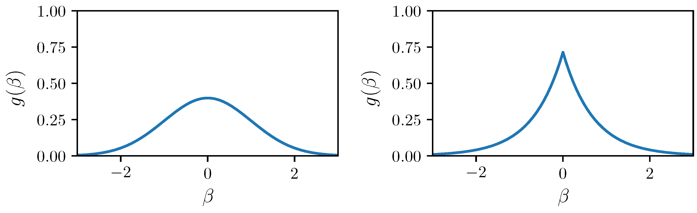
2.7. Bayesian Ridge Regression

BRR is a linear regression technique that integrates Bayesian principles into the determination of model parameters. The method assumes that the coefficients of the regression model adhere to a Gaussian distribution with a zero mean and a precision parameter (inverse of the variance), which is estimated from the data. The incorporation of Bayesian principles into ridge regression is designed to mitigate overfitting by introducing a regularization term [24]. The model can be represented as follows [17]:

$$\begin{array}{c}t=\mathit{\beta }\mathbf{w}+\vartheta \end{array}$$

(7)

where t corresponds to the dependent variable, $\mathit{\beta }$ denotes the coefficient vector, $\mathbf{w}$ represents the independent variable, and $\vartheta$ stands for the error term, which is assumed to follow a Gaussian distribution. The BRR model introduces a prior distribution over $\mathit{\beta }$ and estimates the posterior distribution using Bayesian inference. The regularization term in this model helps in controlling model complexity, making it less prone to overfitting. BRR offers several advantages over traditional linear regression and ridge regression:

• Effective Handling of Multicollinearity: BRR incorporates a regularization term, which is essentially a penalty for large coefficients. This helps to shrink the coefficients of correlated features, making them more stable and less sensitive to small changes in the data [17].
• Prevention of Overfitting: BRR’s shrinkage mechanism effectively reduces overfitting by preventing the model from overemphasizing specific features [25].
• Automatic Shrinkage: BRR automatically determines the optimal degree of shrinkage based on the data, reducing the need for manual tuning of the ridge parameter.

Hastie et al. [26] discuss the applicability of LASSO regression for automatic feature selection, where certain features are deemed irrelevant by setting their coefficients to zero. This highlights a fundamental difference between LASSO and BRR when estimating joint probability distributions. While LASSO tends to eliminate certain coefficients, BRR assumes that all features contribute to some extent, resulting in coefficients rarely reaching zero.

As a graphical example, we tackle the matter from a Bayesian perspective by employing a linear model with normal errors, integrating it with a particular prior distribution for $\beta$. For ridge regression [27], the prior follows a Gaussian distribution with mean zero and a standard deviation determined by $\lambda$. Conversely, for LASSO [23], the distribution is a Laplacian distribution with mean zero and a scale parameter determined by $\lambda$. Figure 2 presents a comparison of the posterior mode of $\beta$ under a Gaussian prior and a Laplacian prior. With LASSO, the prior distribution peaks at zero, indicating an expectation (a priori) that many coefficients $\beta$ will be exactly equal to zero. In contrast, for ridge regression, the prior distribution is flatter at zero, implying an expectation of coefficients to be normally distributed around zero. For further information on BRR, readers can consult the works [17,24], which offer comprehensive discussions of Bayesian Ridge Regression.

2.8. Privacy Analysis

User privacy is maintained by asserting the privacy of local randomizers, which each user applies independently to data records. Local perturbation of a specific attribute can achieve $ϵ$-LDP, where $\epsilon =2hln\left(\frac{2-f}{f}\right)$, with h being the number of hash functions in the Bloom filter and f the flip bit probability. According to the sequential composition theorem [28], the local transformation of a d-dimensional data record achieves ${ϵ}_d$-LDP, where:

$$\begin{array}{c}{ϵ}_d=2dhln\frac{2-f}{f},\end{array}$$

with d representing the number of attributes in the original data record. As all users independently perform the same transformation, the aforementioned ${ϵ}_d$-LDP guarantee is applicable to all distributed users.

3. Proposed Scheme

3.1. Model Definition of Bayesian Ridge Regression (M,y)

This section focuses on demonstrating how we apply BRR using the available data on the server to estimate joint distributions. The server has a vector $\mathbf{y}=(y_1\left[1\right]\cdots y_1\left[k\right])$ originally computed by Equation (5) and a candidate bit matrix $M={({\mathcal{H}}_1\left({\mathsf{\Omega }}_1\right)\times \cdots \times {\mathcal{H}}_k\left({\mathsf{\Omega }}_k\right))}^T$ computed by Equation (6), where k is dimensionality of joint probability distribution estimation. The output parameter is the candidate bit matrix M, and the input feature is the vector $\mathbf{y}$. Substituting the output and input parameters into Equation (7), we have $M=\mathit{\beta }\mathbf{y}+\vartheta$.

3.2. Bayesian Ridge Distribution Estimation

We aim to improve the performance of the LOPUB algorithm by using perturbed Bloom filters as representative features of the data, similar to LOPUB. The central server receives samples with noise from a specific distribution, which can be estimated using linear regression $M=\mathit{\beta }\mathbf{y}+\vartheta$. The candidate bit matrix M is created using Bloom filters, which guarantee that the features extracted by the central server will be the same as those extracted by the user. BRR Algorithm 2 unfolds through a sequence of steps. Initially, the central server acquires perturbed Bloom filters sent by users. Subsequently, the server undertakes the computation of the original count for each bit within k attributes, estimating the accurate count for each. Following this, a candidate bit matrix M is meticulously constructed for k attributes, as illustrated in Figure 1. The BRR model is then fitted, employing the Bloom filters M and the associated counts $\mathbf{y}$. Finally, the probability of the target is determined by normalizing $\mathit{\beta }$, the estimated coefficients derived from the regression model, through division by their sum. Algorithm 2 improves performance and privacy preservation by using perturbed Bloom filters as representative features and by estimating the distribution using BRR.

Algorithm 2 Bayesian Ridge Regression k-way Joint Probability Distributions

$U_j$: jth attribute ($1\le j\le k$)

${\mathsf{\Omega }}_j$: domain of ($1\le j\le k$)

${\widehat{s}}_j^i$: perturbed bloom filter ($1\le i\le N$) ($1\le j\le k$)

f: flipping probability

$\mathcal{H}$: set of hash functions for $U_j$

D: a subset of attributes $U_{j1},\dots ,U_{jk}$

$P_r\left(A_D\right)$: joint probability distribution of k attributes specified by D

for  $eachj\in D$  do

for $eachb=1,\dots ,m_j$ do

compute ${\widehat{y}}_j\left[b\right]={\sum }_{i=1}^N{\widehat{s}}_j^i\left[b\right]$

compute $y_j\left[b\right]=({\widehat{y}}_j\left[b\right]-fN/2)/(1-f)$

end for

${\mathcal{H}}_j\left({\mathsf{\Omega }}_j\right)$ Bloom filters are constructed by the server using $\mathcal{H}$

end for

$\mathbf{y}=(y_1\left[1\right],\dots ,y_1\left[m_1\right]\dots y_k\left[1\right],\dots ,y_k\left[m_k\right])$

$M=({\mathcal{H}}_1\left({\mathsf{\Omega }}_1\right)\times \dots \times {\mathcal{H}}_k\left({\mathsf{\Omega }}_k\right))$ Candidate bit matrix is created

$\mathit{\beta }=BayesianRidgeRegression(M,\mathbf{y})$

return  $P_r\left(A_D\right)=\mathit{\beta }/\sum \mathit{\beta }$

4. Experiments

All experiments were conducted on a machine equipped with an AMD EPYC 7543P 32-Core Processor running at 2.8 GHz and 512 GB of RAM. The machine operated using the Ubuntu 22.04.3 operating system and Python 3.11. For each dataset available in this study, individual data records were examined and locally transformed into noisy Bloom filters as outlined in Section 2.5.1 and Section 2.5.2. Subsequently, the central server estimated the joint probability distribution using Algorithm 2.

4.1. Experimental Method

We applied our approach to fifteen open datasets, namely, seven from the healthcare domain and eight from various sectors, including finance, travel, and others. The following is a brief summary of each dataset used in our experiments.

• The US Census (1990) dataset [29] is a raw dataset extracted from the Public Use Microdata Samples person records. Recognized for its widespread usage, this dataset holds significance for evaluating the efficacy of both CDP and LDP approaches. In our experiments, we opt to utilize 10% of the available users within the dataset, considering the substantial scale of available users. The continuous attributes within the dataset have been discretized into five distinct categories.
• The Bank dataset [30] has the information for marketing campaigns. Through a discretization process, the dataset has been transformed, converting its continuous attributes into five distinct categories.
• The Adult dataset [31] stands out as one of the most widely utilized datasets for assessing the efficacy of CDP and LDP approaches. The continuous attributes within the dataset have been discretized into ten distinct categories.
• The Ms Fimu dataset [32] concerns multiple tourism statistics of the frequency of visitors by days and by the union of consecutive days. The continuous attributes within the dataset have been discretized into five distinct categories.
• The Nursery dataset [33] is derived from a decision model originally developed to rank applications for nursery schools in the 1980s. The dataset has discretized its continuous attributes into ten distinct categories.
• The Diabetes, Stroke, and Hypertension datasets belong to the Behavioral Risk Factor Surveillance System (BRFSS) 2015 [34]. The dataset has undergone a discretization process, resulting in the transformation of its continuous attributes into ten distinct categories.
• The NHANES dataset [35] was used in the PWS Cup 2021 [36], the goal of which was to provide anonymized healthcare data. Through a discretization process, the dataset has been transformed, converting its continuous attributes into ten distinct categories.
• The Cirrhosis dataset [37] compiles information gathered during a Mayo Clinic trial of primary biliary cirrhosis of the liver. The continuous attributes within the dataset have been discretized into ten distinct categories.
• The Lung Cancer dataset [38] comprises information on individuals diagnosed with lung cancer, encompassing various factors such as age, gender, exposure to air pollution, and alcohol consumption. The continuous attributes within the dataset have been discretized into ten distinct categories.
• The Skin Cancer dataset [39] encompasses a summary of dermatoscopic images. Organized in a tabular format, the dataset includes a comprehensive collection of crucial diagnostic categories for pigmented lesions. The dataset has undergone a discretization process, resulting in the transformation of its continuous attributes into ten distinct categories.
• The NIST [40] Privacy Engineering Program introduced National, Texas, and Massachusetts datasets, initiating the Collaborative Research Cycle (CRC) to stimulate research, innovation, and comprehension of data deidentification techniques. These datasets have undergone a discretization process, resulting in the transformation of its continuous attributes into ten distinct categories.

In our experiments, we convert categorical variables into numerical representations using techniques such as Label Encoding, where each category is assigned a unique numerical value. The order of these values is determined alphabetically. We utilize LabelEncoder from the scikit-learn library [41] in Python. It is important to note that the order of numerical values based on the alphabetical order of categories is independent of estimation accuracy. The arrangement is solely determined by the alphabetical sequence of the categories and does not reflect any hierarchy or ranking based on the precision of estimations within those categories.

Table 3 provides a thorough examination of datasets, incorporating key features such as the attribute count, the number of users, and AAR. To compute the AAR, we require the absolute value of the Pearson correlation coefficient $|r_{lt}|$, where $r_{lt}$ is the Pearson correlation coefficient between attributes l and t. The absolute value of $|r_{lt}|$ measures the strength of the linear relationship between two attributes, irrespective of the direction (positive or negative). The average absolute Pearson correlation coefficient for a dataset with j attributes is calculated as

$$\begin{array}{c}AAR=\frac{{\sum }_{l=1}^{j-1}{\sum }_{t=l+1}^j\left|r_{lt}\right|}{\left(\genfrac{}{}{0pt}{}{j}{2}\right)}.\end{array}$$

Here, $\left(\genfrac{}{}{0pt}{}{j}{2}\right)$ is the binomial coefficient representing the number of unique pairs of j attributes. The datasets vary significantly in terms of the number of users, attributes, and average attribute correlation. The US CENSUS dataset has the highest number of users and attributes, with a relatively high AAR of 0.1607. The Cirrhosis dataset has a notably high AAR of 0.2790, indicating stronger correlations among its attributes. The Nursery dataset has the lowest AAR at 0.0411, suggesting weaker correlations among its attributes.

The default parameters are outlined as follows: The number of hash functions employed is denoted as $h=4$, ensuring a consistent false-positive probability of $p=0.022$ across all datasets. This is computed by solving for p in Equation (3) with $m_j=8$ and $|{\mathsf{\Omega }}_j|=2$. The value of $m_j$ varies based on the cardinality of $U_j$ within the datasets and can be computed using Equation (3). We evaluate the performance of three approaches: the simple LOPUB, which relies solely on LASSO regression, the standard LOCOP, and BRR.

Table 3. Datasets characteristics.

Dataset	# Users	# Attributes	AAR
Nursery	12,960	9	0.0240
Lung Cancer	53,427	5	0.0411
Stroke	40,910	11	0.0645
NHANES	4189	10	0.0747
Bank	45,211	17	0.0919
National	27,253	24	0.1002
Massachusets	7634	24	0.1006
Texas	9276	24	0.1035
MS FIMU	88,935	6	0.1068
Adults	45,222	10	0.1088
Hypertension	26,083	14	0.1237
Skin Cancer	10,015	5	0.1268
Diabetes	70,692	18	0.1334
US CENSUS	245,828	68	0.1607
Cirrhosis	418	17	0.2790

Table 3. Datasets characteristics.

Dataset	# Users	# Attributes	AAR
Nursery	12,960	9	0.0240
Lung Cancer	53,427	5	0.0411
Stroke	40,910	11	0.0645
NHANES	4189	10	0.0747
Bank	45,211	17	0.0919
National	27,253	24	0.1002
Massachusets	7634	24	0.1006
Texas	9276	24	0.1035
MS FIMU	88,935	6	0.1068
Adults	45,222	10	0.1088
Hypertension	26,083	14	0.1237
Skin Cancer	10,015	5	0.1268
Diabetes	70,692	18	0.1334
US CENSUS	245,828	68	0.1607
Cirrhosis	418	17	0.2790

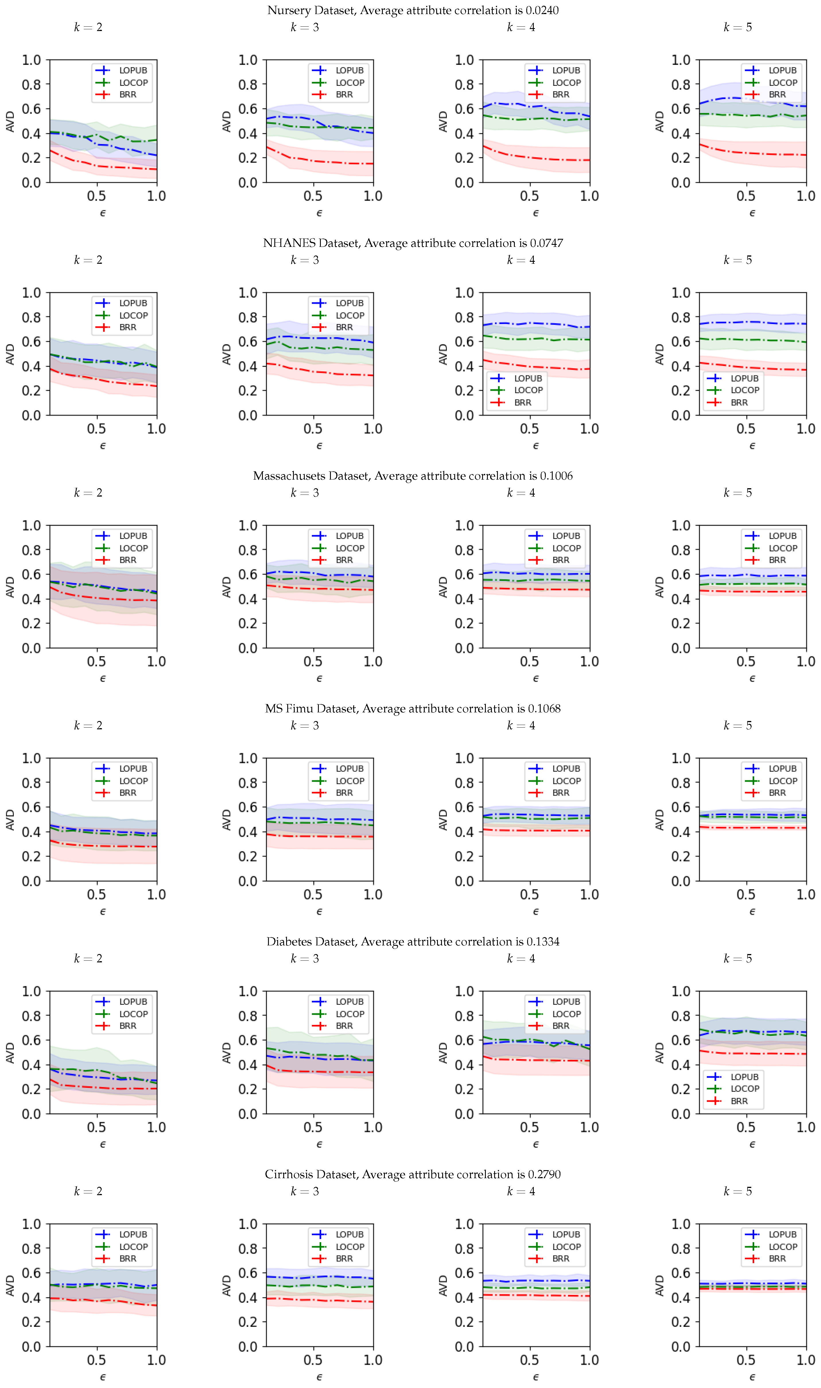
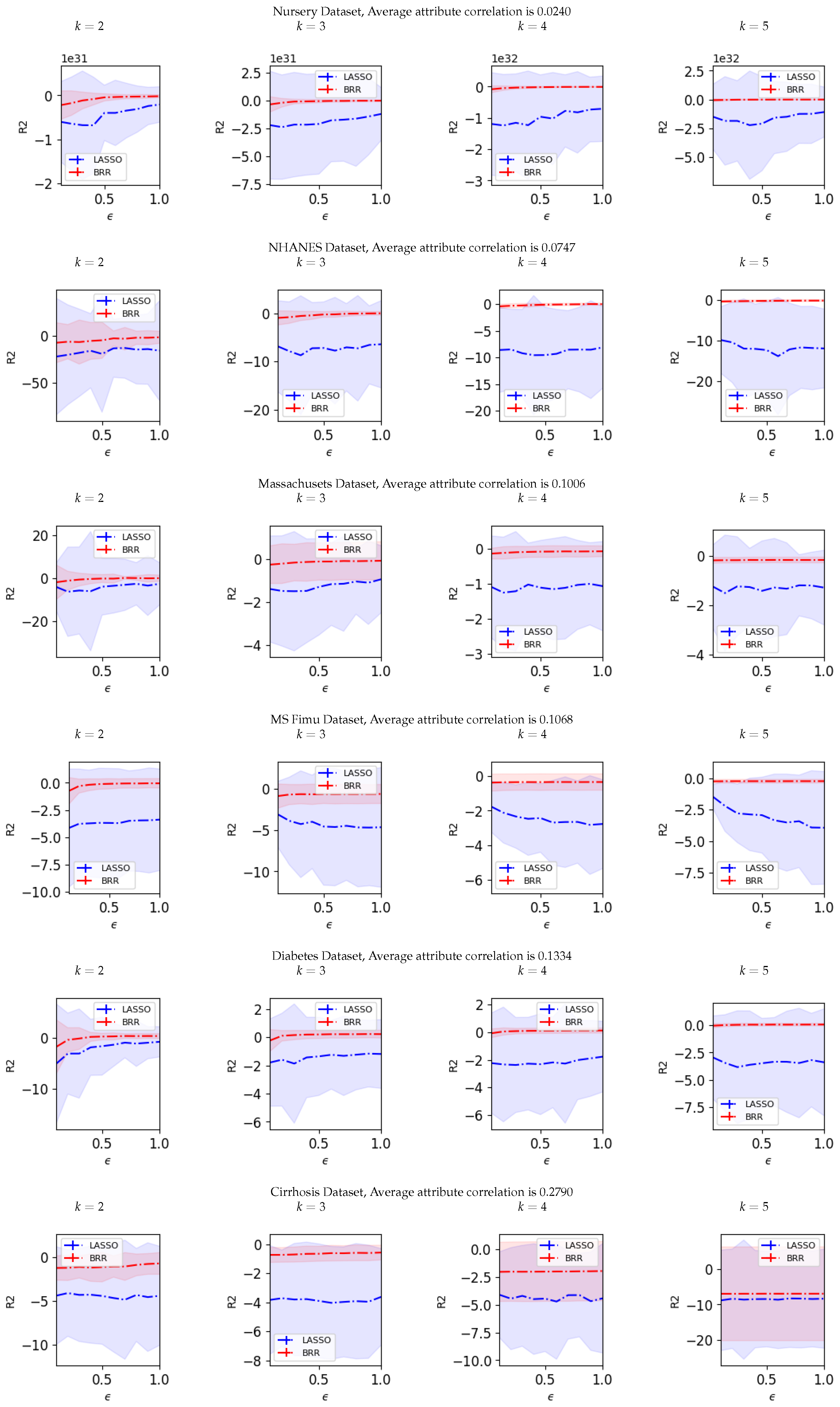
4.2. Results

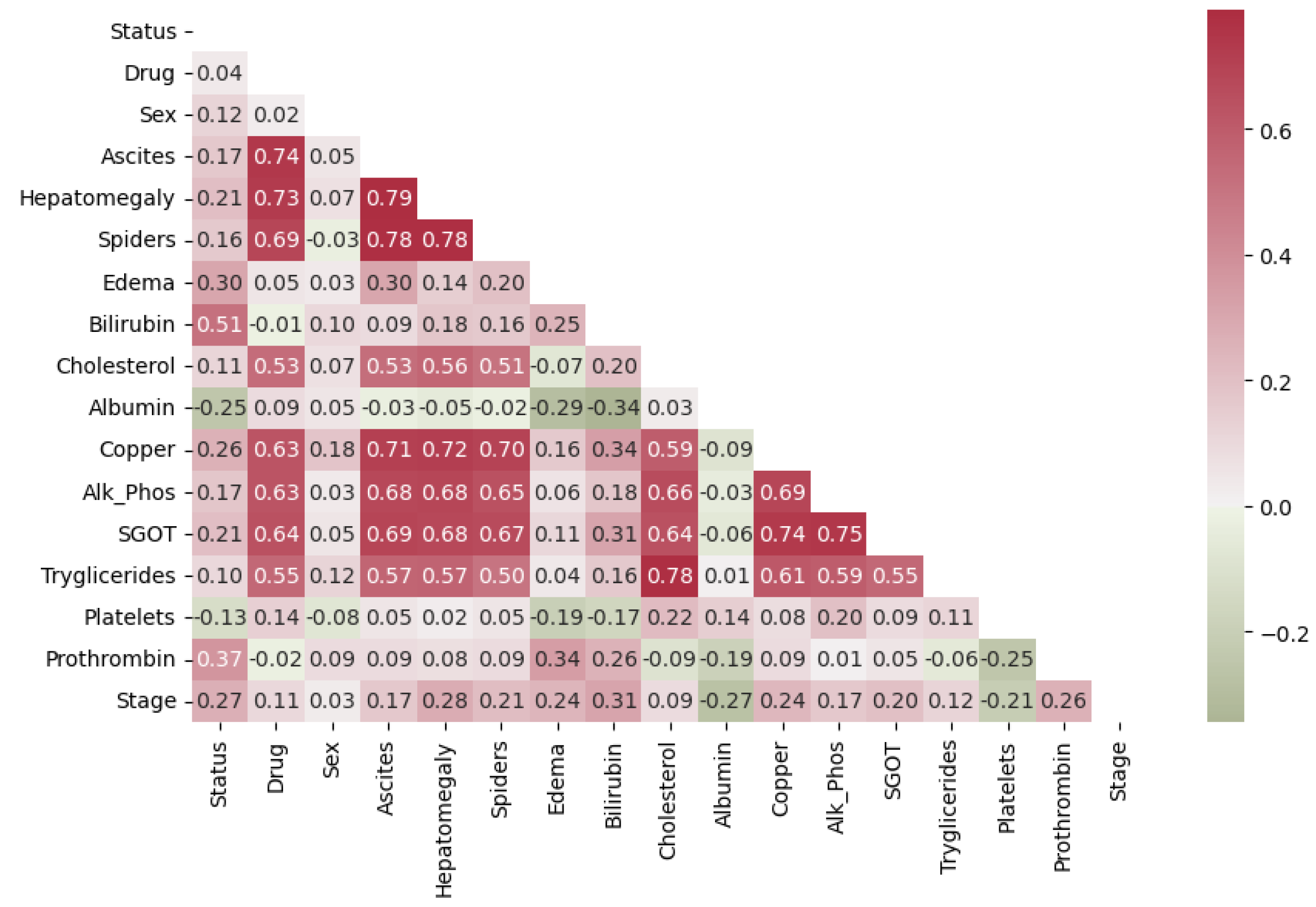
Joint Probability

We select randomly one hundred times k-way joint probability attributes. To analyze the joint probability distributions, we use the AVD to quantify the difference between real and computed data; according to LOPUB [6] and LOCOP [10], it is defined as

$$\begin{array}{c}AVD=\frac{1}{2}\sum _{\omega \in \mathsf{\Omega }}|P\left(\omega \right)-Q\left(\omega \right)|.\end{array}$$

(8)

The results depicted in Figure 3 pertain to six distinct datasets: Nursery, NHANES, Massachusetts, MSFimu, Diabetes, and Cirrhosis. We have chosen to present their results due to the datasets showcasing significant differences in terms of size, attribute composition, and AAR. These variations in size, attribute count, and AAR underscore the diverse nature and potential applications of each dataset across various domains, including healthcare, demographics, and machine learning research. Readers are encouraged to explore the results of the fifteen datasets available in this study by visiting the website https://www.kikn.fms.meiji.ac.jp/~andres/BRR.html, accessed on 27 February 2024. The website also presents a comparison between AVD and AAR for all datasets using different values of $ϵ$ within the range of $[0.1,1]$, along with the k-way joint probability distribution. Figure 4 illustrates the outcomes for $ϵ=0.1$ and $k=2,3,4,5$. We have chosen this specific privacy budget as it provides a robust level of privacy for the users.

Figure 3 presents the results of the experiments conducted on the six datasets using three algorithms: LOPUB, LOCOP, and BRR. The Y-axis illustrates the AVD between the original and computed data, with lower values indicating superior performance. On the X-axis, the privacy budget is depicted, where lower values signify a higher level of privacy. The four columns display results for different k-way settings, specifically $k=2,3,4,5$. The shaded blue, green, and red areas represent the standard deviations of LOPUB, LOCOP, and BRR, respectively.

The findings indicate that, in terms of AVD, BRR consistently outperforms LOPUB and LOCOP. Across all six datasets, BRR achieves lower AVD values than LOPUB and LOCOP at various privacy budgets. This implies that BRR can attain better accuracy while preserving greater privacy compared to the other two algorithms. Overall, the standard deviations are similar for the three algorithms. Moreover, the results reveal an overall enhancement in the performance of all three algorithms as the privacy budget increases. This is attributed to a larger privacy budget allowing users to incorporate less noise for data protection. However, it is crucial to acknowledge that the algorithm performance may vary depending on the dataset. For example, BRR significantly outperforms LOPUB and LOCOP on the Nursery dataset, while the distinction is less pronounced on the Cirrhosis dataset, potentially due to AAR. A high AAR value suggests a strong correlation between attributes, posing a risk of information extraction from one attribute to another or causing noise propagation to other attributes. This, in turn, leads to a further decline in data utility. The propagation of noise makes it difficult to accurately estimate joint probability distributions, as shown in Figure 3.

Figure 5 shows the results of the experiments on the six datasets using two regression algorithms: LASSO and BRR. The Y-axis shows the R-squared between the original and the estimated data, where a value close to one indicates better performance. The X-axis shows the privacy budget, where lower values indicate more privacy. The four columns display results for different k-way joint probability distribution settings, specifically $k=2,3,4,5$. The shaded blue and red areas represent the standard deviation of LASSO and BRR, respectively. BRR generally outperforms LASSO in terms of R-squared. Across all six datasets and privacy budgets, BRR consistently achieves higher R-squared values compared to LASSO. This indicates that BRR effectively handles multicollinearity, even when privacy requirements are stringent. Additionally, it is worth noting that, overall, the standard deviation of LASSO is typically higher than that of BRR. The performance of AVD improves with a decreased privacy budget. As the privacy budget decreases (moving towards the right on the X-axis), the R-squared values for both algorithms increase. This is because a lower privacy budget allows the algorithms to use more information without noise for estimation, leading to better preservation of attributes relationships. BRR’s advantage is most pronounced on the Nursery and MS FIMU datasets. For these datasets, BRR achieves significantly higher R-squared values compared to LASSO, even at low privacy budgets. The difference between BRR and LASSO is smaller on the Cirrhosis dataset. On this dataset, BRR’s R-squared values are only slightly higher than those of LASSO, particularly at $k=5$.

Figure 4 shows the results of the experiments comparing the performance of LOPUB, LOCOP, and BRR on fifteen datasets. The Y-axis shows the AVD between the original and the estimated data, where a value close to zero indicates better performance. The X-axis shows the AAR, where lower values indicate less correlation between attributes. The charts display results for different k-way joint probability distribution settings, specifically $k=2,3,4,5$ with a privacy budget set as $ϵ=0.1$.

Figure 4 shows that BRR generally outperforms LOPUB and LOCOP in terms of utility (AVD). Across $k=4,5$ settings and for most of the datasets, BRR achieves lower AVD values compared to the other two algorithms. This means that BRR can estimate the data more accurately while preserving more privacy than LOPUB and LOCOP.

The performance of all three algorithms varies depending on the dataset. Considering the Nursery and Cirrhosis datasets, which have the lowest and highest AAR values, respectively, in the Nursery dataset, as k increases, BRR significantly outperforms both LOPUB and BRR. In the Cirrhosis dataset, as k increases, the three algorithms exhibit similar values. This suggests that with an increase in k, more highly correlated attributes become available to estimate the joint probability distribution. In Figure 4, the chart in the bottom right, when $k=5$, illustrates how the performances of all three algorithms become similar as highly correlated attributes become available to estimate the joint probability distribution.

For some datasets, such as the Nursery and Bank datasets, BRR achieves significantly lower AVD values compared to the other algorithms. However, for other datasets, such as the Cirrhosis and USCENSUS datasets, the differences between the algorithms are smaller. BRR’s advantage is most pronounced for $k=4,5$. For these settings, BRR consistently achieves the lowest AVD values across most datasets. LOPUB generally performs worse than LOCOP and BRR. Across all k-way settings and most datasets, LASSO has the highest AVD values among the three algorithms.

Figure 4 illustrates how the health datasets exhibit a rightward skew on the X-axis, with the Cirrhosis dataset having the highest AAR. This dataset contains information related to patients with primary biliary cirrhosis who participated in a clinical trial conducted by the Mayo Clinic [37].

Figure 6 shows the correlation matrix for the Cirrhosis dataset; for example, sex and ascites demonstrate a weak positive correlation (0.12), suggesting a slight tendency for one to increase as the other does. Ascites and edema show a moderate positive correlation (0.30), implying a stronger association. Bilirubin and albumin exhibit a moderate negative correlation (−0.25), meaning as bilirubin levels rise, albumin levels tend to decrease. Copper and alkaline phosphatase (Alk Phos) have a moderate positive correlation (0.71), indicating a notable relationship where they increase or decrease together. SGOT (an enzyme found in the liver) and Alk Phos also display a moderate positive correlation (0.68). Finally, platelets and prothrombin have a weak negative correlation (−0.13), hinting at a slight inverse relationship between the two. We can now explore more generally the potential correlations between the attributes available in the cirrhosis disease [42].

• Sex, categorized as male or female, could be correlated with various health parameters and responses to treatment.
• Ascites, hepatomegaly, and spiders are variables indicating the presence or absence of certain clinical features. Correlations with other health parameters, especially liver-related ones, may exist.
• Bilirubin, cholesterol, albumin, copper, alkaline phosphatase, SGOT, triglycerides, platelets, and prothrombin are laboratory measurements indicating different aspects of a patient’s health. Examining correlations among these variables may unveil concealed patterns associated with physiological processes, such as liver function and blood composition.

While a healthcare professional can provide a more in-depth analysis of the necessity of each variable in this dataset, it is crucial to highlight that highly correlated attributes may raise privacy concerns when sharing data with third parties. Additionally, introducing noise to one attribute can result in the propagation of noise to other attributes, leading to a further decline in data utility. This noise propagation makes it challenging to accurately estimate joint probability distributions, as depicted in Figure 4, where the results indicate that the AVD generally increases as the value of k increases.

Figure 6. Correlation matrix for the Cirrhosis dataset.

Figure 6. Correlation matrix for the Cirrhosis dataset.

5. Discussion

We conducted a comprehensive evaluation of datasets across various domains, employing our proposed LDP scheme based on BRR, across various scenarios involving $k=2,3,4,5$ with a privacy budget set at 0.1. Regrettably, direct comparison with the study conducted by Arcolezi et al. [2] is not feasible, although both methods employ LDP. Their main objective revolves around improving accuracy in machine learning models, whereas our emphasis is on estimating the joint probability distribution with minimal error.

Our proposed method consistently outperforms LOPUB and LOCOP across various datasets, considering differences in size, attribute composition, and the average absolute Pearson correlation coefficient (AAR). The AAR serves as a valuable tool for scrutinizing datasets prior to publication and evaluating the performance of synthetic data algorithms. This preventive approach helps avoid the release or sharing of datasets containing highly correlated attributes, thereby safeguarding the privacy of users within the dataset. For instance, this paper assesses the performance using the Nursery and Cirrhosis datasets, showcasing the lowest and highest AAR values, respectively. Our findings indicate that as k increases, more highly correlated attributes become available for estimating the joint probability distribution, posing a risk, especially in the absence of a small privacy budget, which implies robust privacy protection.

Particularly noteworthy is a specific dataset (the dataset with a lower AAR) where our method achieved a remarkable decrease in the average variant distance compared to LOPUB and LOCOP. Additionally, for the other datasets, our proposed method outperformed the well-known LOPUB and LOCOP algorithms, both based on randomized response and the LASSO algorithm, with a privacy budget set at 0.1 per attribute and $k=5$.

Continuing our experiments, we employ the R-squared metric to assess the performance of LASSO and Bayesian Ridge Regression. The findings reveal that BRR consistently outperforms both LOPUB and LOCOP, both of which are based on LASSO regression. These results illustrate how BRR exhibits greater stability across various k-way evaluations, privacy budgets, and AAR compared to LASSO, owing to its effective handling of multicollinearity. In summary, our study unveils the nuanced performance of our proposed method, LOPUB, and LOCOP across diverse datasets, emphasizing the crucial influence of AAR on their efficacy. These findings underscore the necessity of aligning algorithmic choices with the unique characteristics of datasets to achieve optimal results. These insights hold significant implications for applications such as healthcare, where precise predictions and considerations of attribute correlations are paramount. Importantly, our study underscores the importance of avoiding high correlation among attributes in datasets, as revealed by our results.

Highly correlated attributes in a dataset present two risks. Firstly, information from one attribute can be inferred from another, compromising the privacy guarantees provided by local differential privacy, especially when working with a high privacy budget value. Secondly, when employing a small privacy budget value in a dataset with highly correlated attributes, introducing noise to one attribute can cause the noise to propagate to other attributes. This propagation of noise results in a further decline in data utility. It becomes challenging to accurately estimate joint probability distributions, particularly for higher values of k-way.

5.1. Curse of Dimensionality

The curse of dimensionality presents a significant obstacle within LDP. LDP aims to protect privacy by injecting noise into individual data points before sharing. However, as data dimensionality grows, the volume of noise needed to obscure true values while upholding the same privacy standards increases dramatically. This results in a loss of data utility.

Our experiments depicted in Figure 5 illustrate a noticeable trend of declining performance, as evidenced by an increased AVD, with higher k values. This highlights the trade-off between accuracy and dimensionality, underscoring the challenges associated with the curse of dimensionality. Notably, our proposed method exhibits lower AVD values, indicating superior data utility compared to LOPUB and LOCOP, especially for datasets with an AAR close to zero.

5.2. Real-World Applicability of the Proposed Method

The proposed LDP scheme based on BRR holds significant potential for revolutionizing data analysis in the healthcare industry while ensuring the utmost protection of patient privacy. LDP techniques enable healthcare organizations to conduct data analysis, such as epidemiological studies and treatment outcome analysis, without compromising patient privacy. Additionally, LDP provides a secure framework for data sharing, allowing collaboration on initiatives like population health management and clinical trials while safeguarding patient information. Moreover, LDP facilitates personalized medicine by analyzing patient-specific data while preserving confidentiality. Integration of LDP into healthcare analytics and machine learning models enables predictive analysis and proactive decision-making without exposing individual patient data. Furthermore, LDP enhances the privacy and security of telemedicine and remote patient monitoring systems, ensuring patient confidentiality in virtual healthcare settings. Overall, LDP has the potential to transform healthcare data analysis while maintaining patient privacy and confidentiality.

Unfortunately, direct comparison with the Sung et al. [16] study is not feasible, despite both methods applying LDP to medical data. Their primary objective lies in enhancing accuracy in machine learning models, while our focus centers on estimating the joint probability distribution with minimal error.

6. Conclusions

This paper presents a comprehensive evaluation of datasets spanning various domains. We employed our proposed LDP scheme based on BRR across different scenarios while estimating the joint probability distribution with a privacy budget set at 0.1. Our method consistently outperformed LOPUB and LOCOP. We suggest using the average absolute Pearson correlation coefficient (AAR) as a valuable tool for scrutinizing datasets before publication and assessing the performance of synthetic data algorithms. This approach helps prevent the release or sharing of datasets containing highly correlated attributes, safeguarding users’ privacy. Particularly in datasets with a lower AAR, our method achieved a significant decrease in the average variant distance compared to LOPUB and LOCOP.

We utilized the R-squared metric to evaluate the performance of LASSO regression and Bayesian Ridge Regression. The results demonstrate that BRR consistently outperforms both LOPUB and LOCOP, which are based on LASSO regression. This highlights BRR’s greater stability across various joint probability distribution evaluations, privacy budgets, and AAR compared to LASSO, thanks to its effective handling of multicollinearity.

In summary, our study reveals the nuanced performance of our proposed method, LOPUB, and LOCOP across diverse datasets, underscoring the significant influence of AAR on their efficacy. These findings stress the importance of aligning algorithmic choices with datasets’ unique characteristics to achieve optimal results, especially in critical applications like healthcare, where precise predictions and considerations of attribute correlations are crucial. Importantly, our study highlights the need to avoid high correlation among attributes in datasets, as indicated by our results.

In contemplating the future of this research, we anticipate a continuous process of refining and optimizing our proposed LDP scheme based on BRR. This entails addressing the intricate trade-off between accuracy and computational complexity across diverse scenarios, which includes variations in privacy budgets and attribute compositions. We envision further advancements aimed at enhancing the adaptability and efficacy of our approach in real-world applications. Additionally, we aim to extend the application of our LDP approach to generate accurate machine learning models.

The importance and contribution of this work for the future are substantial. Our results demonstrate that BRR is able to present better performance than LOPUB and LOCOP when a strong privacy budget is used to protect the privacy of the users. These findings suggest that BRR can be an effective tool for privacy preservation in data publication, and it may have various applications where privacy is a concern.

References

- Dwork, C.; Roth, A. The Algorithmic Foundations of Differential Privacy. Found. Trends Theor. Comput. Sci. 2014, 9, 211–407. [Google Scholar] [CrossRef]
- Arcolezi, H.H.; Makhlouf, K.; Palamidessi, C. (Local) Differential Privacy has NO Disparate Impact on Fairness. In Data and Applications Security and Privacy XXXVII; Atluri, V., Ferrara, A.L., Eds.; DBSec 2023. Lecture Notes in Computer Science; Springer: Cham, Switzerland, 2023; Volume 13942. [Google Scholar] [CrossRef]
- Yang, M.; Guo, T.; Zhu, T.; Tjuawinata, I.; Zhao, J.; Lam, K.Y. Local differential privacy and its applications: A comprehensive survey. Comput. Stand. Interfaces 2023, 89, 103827. [Google Scholar] [CrossRef]
- Erlingsson, Ú.; Pihur, V.; Korolova, A. RAPPOR: Randomized Aggregatable Privacy-Preserving Ordinal Response. In Proceedings of the 2014 ACM SIGSAC Conference on Computer and Communications Security, Scottsdale, AZ, USA, 3–7 November 2014; Association for Computing Machinery: New York, NY, USA, 2014. ISBN 9781450329576. [Google Scholar]
- Mac Apple. Differential Privacy Technical Overview. Available online: https://www.apple.com/privacy/docs/Differential_Privacy_Overview.pdf (accessed on 26 November 2022).
- Ren, X.; Yu, C.M.; Yu, W.; Yang, S.; Yang, X.; McCann, J.A.; Philip, S.Y. LoPub: High-Dimensional Crowdsourced Data Publication with Local Differential Privacy. IEEE Trans. Inf. Forensics Secur. 2018, 13, 2151–2166. [Google Scholar] [CrossRef]
- Warner, S.L. Randomized Response: A Survey Technique for Eliminating Evasive Answer Bias. J. Am. Stat. Assoc. 1965, 60, 63–69. [Google Scholar] [CrossRef]
- Zou, H.; Hastie, T.; Tibshirani, R. On the “degrees of freedom” of the LASSO. In The Annals of Statistics; Institute of Mathematical Statistics: Hayward, CA, USA, 2007; Volume 35. [Google Scholar]
- Dempster, A.P.; Laird, N.M.; Rubin, D.B. Maximum likelihood from incomplete data via the EM algorithm. J. R. Stat. Soc. Ser. 1977, 39, 1–22. [Google Scholar] [CrossRef]
- Wang, T.; Yang, X.; Ren, X.; Yu, W.; Yang, S. Locally Private High-Dimensional Crowdsourced Data Release Based on Copula Functions. IEEE Trans. Serv. Comput. 2022, 15, 778–792. [Google Scholar] [CrossRef]
- Jiang, X.; Zhou, X.; Grossklags, J. Privacy-Preserving High-dimensional Data Collection with Federated Generative Autoencoder. Proc. Priv. Enhancing Technol. 2022, 2022, 481–500. [Google Scholar] [CrossRef]
- Van Wieringen, W.N. Lecture notes on ridge regression. arXiv 2021, arXiv:1509.09169. Available online: https://arxiv.org/pdf/1509.09169 (accessed on 26 November 2022).
- Sambasivan, R.; Das, S.; Sahu, S.K. A Bayesian perspective of statistical machine learning for big data. Comput. Stat. 2020, 35, 893–930. [Google Scholar] [CrossRef]
- Assaf, A.G.; Tsionas, M.; Tasiopoulos, A. Diagnosing and correcting the effects of multicollinearity: Bayesian implications of ridge regression. Tour. Manag. 2019, 71, 1–8. [Google Scholar] [CrossRef]
- Hernandez-Matamoros, A.; Kikuchi, H. An Efficient Local Differential Privacy Scheme Using Bayesian Ridge Regression. In Proceedings of the 20th Annual International Conference on Privacy, Security and Trust (PST), Copenhagen, Denmark, 21–23 August 2023; pp. 1–7. [Google Scholar] [CrossRef]
- Sung, M.; Cha, D.; Park, Y. Local Differential Privacy in the Medical Domain to Protect Sensitive Information: Algorithm Development and Real-World Validation. JMIR Med. Inform. 2021, 9, e26914. [Google Scholar] [CrossRef]
- Michimae, H.; Emura, T. Bayesian ridge estimators based on copula-based joint prior distributions for regression coefficients. Comput. Stat. 2022, 37, 2741–2769. [Google Scholar] [CrossRef]
- Wang, T.; Zhang, X.; Feng, J.; Yang, X. A Comprehensive Survey on Local Differential Privacy toward Data Statistics and Analysis. Sensors 2020, 20, 7030. [Google Scholar] [CrossRef]
- Chicco, D.; Warrens, M.J.; Jurman, G. The coefficient of determination R-squared is more informative than SMAPE, MAE, MAPE, MSE and RMSE in regression analysis evaluation. PeerJ Comput. Sci. 2021, 7, e623. [Google Scholar] [CrossRef]
- Kasiviswanathan, S.P.; Lee, H.K.; Nissim, K.; Raskhodnikova, S.; Smith, A. What Can We Learn Privately? In Proceedings of the 49th Annual IEEE Symposium on Foundations of Computer Science, Philadelphia, PA, USA, 25–28 October 2008. [Google Scholar]
- Bloom, B.H. Space/Time Trade-Offs in Hash Coding with Allowable Errors. Assoc. Comput. Mach. 1970, 13, 422–426. [Google Scholar] [CrossRef]
- Broder, A.Z.; Mitzenmacher, M. Survey: Network Applications of Bloom Filters: A Survey. Internet Math. 2003, 1, 485–509. [Google Scholar] [CrossRef]
- Santosa, F.; Symes, W.W. Linear inversion of band-limited reflection seismograms. SIAM J. Sci. Stat. Comput. 1986, 7, 1307–1330. [Google Scholar] [CrossRef]
- Tipping, M.E. Sparse bayesian learning and the relevance vector machine. J. Mach. Learn. Res. 2001, 1, 211–244. [Google Scholar] [CrossRef]
- Posch, K.; Arbeiter, M.; Pilz, J. A novel Bayesian approach for variable selection in linear regression models. Comput. Stat. Data Anal. 2020, 144, 106881. [Google Scholar] [CrossRef]
- Hastie, T.; Tibshirani, R.; Friedman, J. The Elements of Statistical Learning: Data Mining, Inference, and Prediction; Springer Science Business Media: New York, NY, USA, 2009. [Google Scholar]
- Tibshirani, R. Regression shrinkage and selection via the lasso. J. R. Stat. Soc. Ser. B Methodol. 1996, 58, 267–288. [Google Scholar] [CrossRef]
- McSherry, F.D. Privacy integrated queries: An extensible platform for privacy-preserving data analysis. In Proceedings of the 2009 ACM SIGMOD International Conference on Management of Data, Providence, RI, USA, 29 June–2 July 2009; pp. 19–30. [Google Scholar]
- Meek Thiesson and Heckerman; US Census Data. UCI Machine Learning Repository. 1990. Available online: https://archive.ics.uci.edu/dataset/116/us+census+data+1990 (accessed on 15 November 2023).
- Rita, P.; Cortez, P.; Moro, S.; Bank Marketing. UCI Machine Learning Repository. Available online: https://archive.ics.uci.edu/dataset/222/bank+marketing (accessed on 15 November 2023).
- Adult. UCI Machine Learning Repository. 1996. Available online: https://archive.ics.uci.edu/dataset/2/adult (accessed on 15 November 2023).
- Arcolezi, H.H.; Couchot, J.-F.; Baala, O.; Contet, J.-M.; Al Bouna, B.; Xiao, X. Mobility modeling through mobile data: Generating an optimized and open dataset respecting privacy. In Proceedings of the 2020 International Wireless Communications and Mobile Computing (IWCMC), Limassol, Cyprus, 15–19 June 2020; pp. 1689–1694. [Google Scholar]
- Rajkovic, V. Nursery. UCI Machine Learning Repository. 1997. Available online: https://archive.ics.uci.edu/dataset/76/nursery (accessed on 15 November 2023).
- CDC. CDC—2015 BRFSS Survey Data and Documentation. 2015. Available online: https://www.cdc.gov/brfss/annual_data/annual_2015.html (accessed on 15 November 2023).
- Kikuchi, H. PWS Cup 2021. Data Anonymization Competition ‘Diabetes’. Available online: https://github.com/kikn88/pwscup2021 (accessed on 26 November 2022).
- PWS. PWS 2021. Available online: https://www.iwsec.org/pws/2021/cup21.html (accessed on 26 November 2022).
- Fleming, T.R.; Harrington, D.P. Counting Processes and Survival Analysis. In Wiley Series in Probability and Mathematical Statistics: Applied Probability and Statistics; John Wiley and Sons Inc.: New York, NY, USA, 1991. [Google Scholar]
- Hong, Z.Q.; Yang, J.Y. Optimal Discriminant Plane for a Small Number of Samples and Design Method of Classifier on the Plane. Pattern Recognit. 1991, 24, 317–324. [Google Scholar] [CrossRef]
- Tschandl, P.; Rosendahl, C.; Kittler, H. The HAM10000 dataset, a large collection of multi-source dermatoscopic images of common pigmented skin lesions. Sci. Data 2018, 5, 180161. [Google Scholar] [CrossRef] [PubMed]
- Collaborative Research Cycle—NIST Pages—National Institute of Standards and Technology, Howarth, Gary, National Institute of Standards and Technology USA. 2023. Available online: https://github.com/usnistgov/privacy_collaborative_research_cycle (accessed on 26 September 2023).
- Pedregosa, F.; Varoquaux, G.; Gramfort, A.; Michel, V.; Thirion, B.; Grisel, O.; Blondel, M.; Prettenhofer, P.; Weiss, R.; Dubourg, V.; et al. Scikit-learn: Machine Learning in Python. J. Mach. Learn. Res. 2011, 12, 2825–2830. [Google Scholar]
- GBD 2017 Cirrhosis Collaborators. The global, regional, and national burden of cirrhosis by cause in 195 countries and territories, 1990–2017: A systematic analysis for the Global Burden of Disease Study 2017. Lancet Gastroenterol. Hepatol. 2020, 5, 245–266. [Google Scholar] [CrossRef] [PubMed]