Characteristics of Electric Field Induced by Oscillating Metal Underwater Vehicle

Abstract

To analyze the induced electric field characteristics generated by the rotation and shaking of underwater metal vehicles, a mathematical model of the induced electric field generated by the underwater metal vehicles was derived using Faraday’s electromagnetic induction law. A mathematical model of the induced electric field on the electrode pairs of metal vehicles shaking in different coordinate system planes was established through in-depth analysis. Based on this, a three-component output model of the induced electric field output by the three-axis sensor was obtained when the measurement system was shaking at all three angles. At a constant speed, the induced electric field interference output by the measurement system is a static signal. The value of the static electric field is proportional to the vehicle’s speed and the value of the geomagnetic field, and the value of each component is related to the direction of movement and the value of the geomagnetic field component. The simulation results show that when the navigation body is moving at a constant speed, the induced electric field is a static electric field with a magnitude of mV/m. In a stable state, the induced electric field noise generated by changes in pitch, roll, and heading sway is at the nV/m level and does not have a significant impact on detection. The correctness of the theoretical model has been verified through experiments on offshore speedboat platforms, and it is feasible to use metal navigation bodies for ship electric field detection.

1. Introduction

As an important source of target exposure, ship electric fields have the advantages of being unable to be completely eliminated, strong anti-interference ability, and obvious line spectrum characteristics. They are often used for underwater target detection and underwater weapon fuses [1,2,3,4,5]. With the escalating conflict of international maritime rights and the progress of countries around the world in ship noise reduction and demagnetization, the detection of electric fields in water targets has attracted much attention. Domestic and foreign research teams have achieved many results in detection, identification, and tracking positioning, greatly enriching the application of underwater electric fields in underwater target detection [6,7,8,9,10,11,12].

In recent years, various types of underwater vehicles such as UUVs(Unmanned underwater vehicleS), AUVs(Autonomous Underwater Vehicle), and underwater gliders have developed rapidly due to their advantages such as low cost, small platform volume, flexible deployment, and strong environmental adaptability [13,14,15,16,17]. Among them, high-speed underwater vehicles such as supercavitating torpedoes, small submarines, high-speed ships, and anti-submarine high-speed ammunition can achieve a basic speed of 100 m/s; their maximum speed can instantly reach underwater sound speed [18]. This type of vehicle can be equipped with various sensors for target detection according to mission requirements, so it is widely used in the military and civil fields.

Underwater vehicles are generally made of metal, and when they move underwater at a uniform speed, the metal hull will inevitably cut the magnetic field lines of the Earth’s magnetic field and generate an electromotive force, which will generate an induced electric field in space. Considering the application platform, the interference generated by its motion mainly has two aspects: one is the platform’s own movement cutting the induced electric potential generated by the geomagnetic field through the seawater to form an induced electric field; the second is that the movement of the platform causes the electric field sensors and wires to cut off the geomagnetic field generated by the induced electric field. Since most metallic moving objects/motion targets are encapsulated in air bubbles during high-speed underwater navigation, the induced electric field formed by their leakage into seawater has relatively little effect on the electric field measurements. This paper focuses on the analysis of the induced electric field generated by wire cutting in the geomagnetic field, including the induced electric field generated by the cutting of the metal moving platform and the induced electric field caused by the vibration of the platform.

The development of underwater vehicles and electric field detection technology provides a new approach for the detection of underwater targets. Combining electric field detection with underwater vehicle detection can achieve better target detection results, fully leveraging the advantages of electric field detection and underwater vehicles. In reference [4], to solve the problems of obtaining electric field signals and detecting targets in deep and distant seas, the electric field detection system was combined with ocean buoys to analyze the interference electric field characteristics of the measured data of deep-sea electric field detection profile buoys. The results showed that the electromagnetic valve of the buoy platform would interfere with the electric field sensors installed nearby. Through the adaptive threshold line spectrum energy sum detection method, the detection probability was high and the false alarm rate was low. Suitable for application on buoy detection platforms, it can fully leverage the advantages of electric field detection and buoy detection. Reference [19] analyzed the measured electric field data of offshore shaking platforms, clarified the characteristics of electric field interference on shaking platforms, and pointed out that it is not suitable to use electrostatic fields or static potential differences as signal sources in ship electric field tracking on offshore shaking platforms. The axial frequency electric field was used as a signal source, and the shaking platform was used to detect and track the axial frequency electric field. The results indicate the effectiveness of the combination of the shaking platform and the electric field detection system in tracking the axial frequency electric field. Unlike underwater buoys or water swaying platforms, there is no domestic underwater vehicle equipped with an electric field detection system, and there is a lack of research on the electric field interference characteristics of the vehicle platform.

2. Mathematical Model of Induced Electric Field for Metal Motion

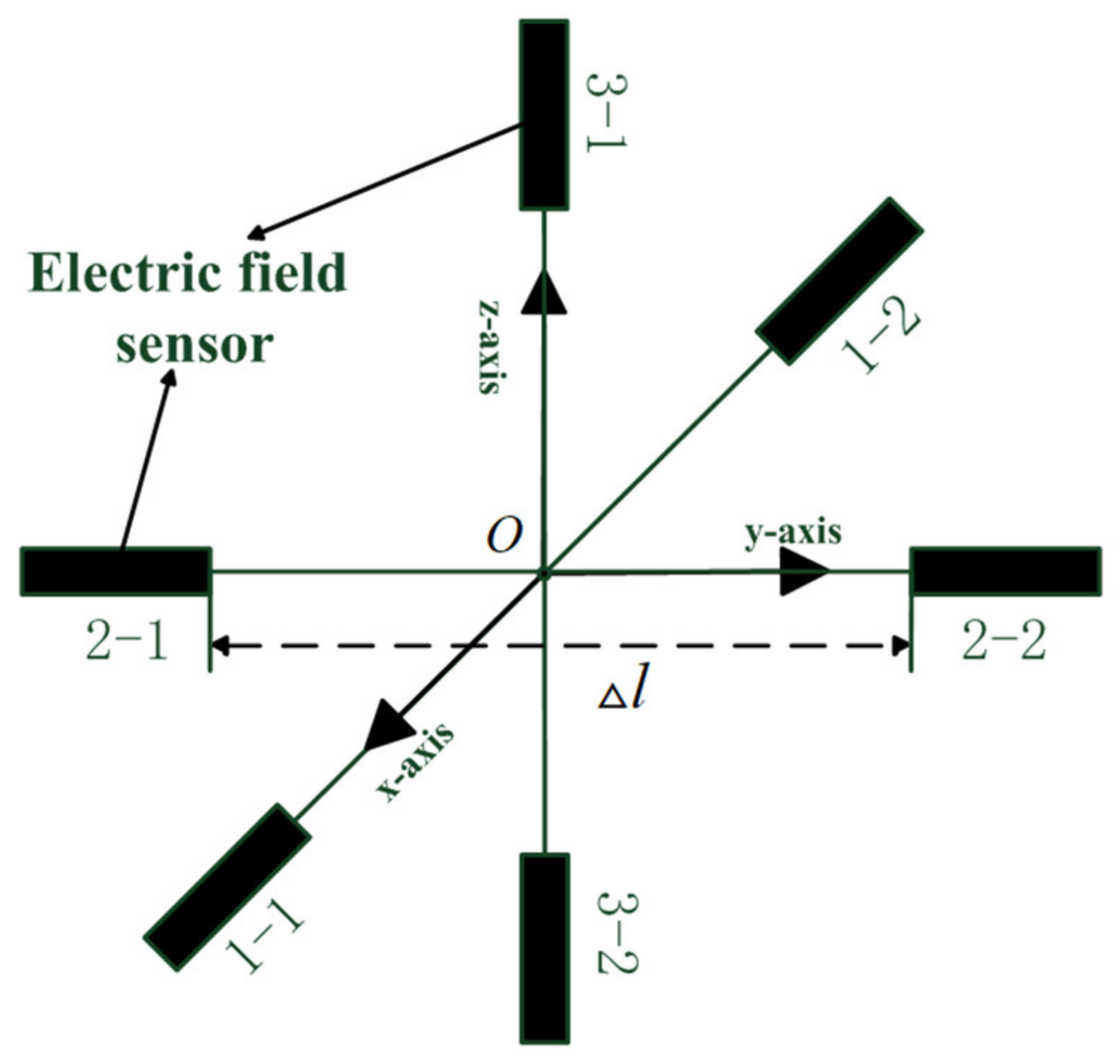
For moving electric field detection platforms such as metal navigation bodies, electric field sensors are fixed on the detection platform. According to the principle of electric field measurement, electric field sensors are arranged in pairs as shown in Figure 1, and orthogonal pairs are used to measure the potential difference between two points. The expression is as follows:

$$E_l=\underset{\Delta l\to 0}{\lim }\frac{U_1-U_2}{\Delta l}$$

(1)

In Equation (1), $\Delta l$ is the distance between electrode pairs, also known as electrode distance; $U_1$ represents the potential measured by sensor 1 in each pair of electric field sensors, and similarly, $U_2$ represents the potential measured by sensor 2 in each pair of electric field sensors; $E_l$ is the electric field between electrode pairs.

According to Equation (1), for electric field measurement, the smaller the electrode distance, the more accurate it is. However, for target detection, the larger the electrode distance, the higher the system sensitivity, and the farther the detection distancecan be achieved. When the motion platform moves, the measurement system electric field sensor and its wire will cut the geomagnetic field and produce induced electromotive force; if the movement speed is constant, the induced electromotive force is a stable static potential difference, which will only affect the measurement of the static electric field or potential and will not have a significant impact on the detection of low-frequency electric fields. The interference electromotive force generated by unstable motion speed or periodic shaking is an alternating signal, which will have an impact on the detection of low-frequency electric fields. The following will be derived separately.

Assume that the measurement systems 1-1 and 1-2 as shown in Figure 1 are oriented along the x-axis, 2-1 and 2-2 along the y-axis, and 3-1 and 3-2 along the z-axis. $\mathit{E}=\mathit{E}(E_x,E_y,E_z)$ is the induced electric field, where $E_x,E_y,E_z$ represents the components along the three directions; the velocity of the probe platform is $\mathit{v}=(v_x,v_y,v_z)$, where $v_x$, $v_y$, and $v_z$ are the velocity components along the three directions, respectively, which are obtained by Faraday’s law of electromagnetic induction:

$$\mathit{E}=\mathit{E}(E_x,E_y,E_z)=\mathit{v}\times {\mathit{B}}_E$$

(2)

In the formula, ${\mathit{B}}_E=(B_x,B_y,B_z)$ is the geomagnetic field, which is substituted into the solution to obtain

$$E_x=v_y{B}_z-v_z{B}_y=-F\left[v_y\sin (I)+v_z\cos (I)\sin (\gamma )\right]$$

(3)

$$E_y=v_z{B}_x-v_x{B}_z=F\left[v_z\cos (I)\cos (\gamma )+v_x\sin (I)\right]$$

(4)

$$E_z=v_x{B}_y-v_y{B}_x=F\left[v_x\cos (I)\sin (\gamma )-v_y\cos (I)\cos (\gamma )\right]$$

(5)

In the above equation, $F$ is the modulus of the geomagnetic field, I is the magnetic inclination angle, and $\gamma$ is the magnetic declination angle (the dip angle I denotes the angle between ${\mathit{B}}_E$ and a plane tangent to Earth; the angle $\gamma$ is the deviation between the magnetic north and the x-axis). Equations (3)–(5) are the electric field obtained from the potential difference of the output of the three-axis measuring system, and it can be seen from the expressions that the electric field is only related to the platform speed and the three components of the geomagnetic field, and it is a static signal that does not change with changes in time.

When the motion detection platform shakes at a certain angle, the measurement system will also shake accordingly. Assume that the angular velocity of the x-y plane shaking, i.e., the rate of change in direction angle, is ${\omega }_d$, the angular velocity of the x-z plane shaking, i.e., the rate of change in pitch angle, is ${\omega }_p$, and the angular velocity of the y-z plane shaking, i.e., the rate of change in roll angle, is ${\omega }_r$.

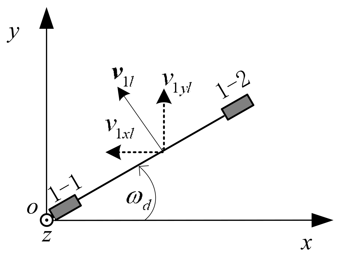
2.1. The Measurement System Shakes in the x-y Plane

The measurement system shakes in the x-y plane, assuming that at time $t=0$, as shown in Figure 1, the three pairs of electric field sensors in the electric field measurement system are aligned with the coordinate axis direction, and 1-1 and 1-2 are on the x-axis; the state over time $t$ is shown in Figure 2. The distance between electrodes 1-1 is located at the coordinate origin, and the linear velocity at the distance from the coordinate origin is ${\mathit{v}}_{1l}={\omega }_{d}l$.

At time $t$, the three components of velocity at $l$ when shaking in the x-y plane can be obtained as follows:

$$v_{1xl}=-{\omega }_{d}l\sin ({\omega }_{d}t)$$

(6)

$$v_{1yl}={\omega }_{d}l\cos ({\omega }_{d}t)$$

(7)

$$v_{1zl}=0$$

(8)

Substituting Equations (6)–(8) into (2), the three components of the electric field at the 1-1 and 1-2 electrode pairs can be obtained as follows:

$$E_{1xl}=v_{1yl}{B}_z-v_{1zl}{B}_y=B_z{\omega }_{d}l\cos ({\omega }_{d}t)$$

(9)

$$E_{1yl}=v_{1zl}{B}_x-v_{1xl}{B}_z=B_z{\omega }_{d}l\sin ({\omega }_{d}t)$$

(10)

$$E_{1zl}=v_{1xl}{B}_y-v_{1yl}{B}_x=-{\omega }_{d}l[B_y\sin ({\omega }_{d}t)+B_x\cos ({\omega }_{d}t)]$$

(11)

Combining Equation (1) shows that the electric field is approximated by the potential difference, which in turn is equal to the integral of the electric field $U={\displaystyle \int E}dl$, so that the induced electric field on the 1-1 and 1-2 electrode pairs when the measurement system is shaking in the x-y plane is

$$\begin{array}{l}{E}_{1d}={\displaystyle {\int }_0^{\Delta l}[E_{1xl}\cos ({\omega }_{d}t)+E_{1yl}\sin ({\omega }_{d}t)}]dl/\Delta l\\ \begin{array}{cc}& =\end{array}{\displaystyle {\int }_0^{\Delta l}{B}_z{\omega }_{d}l}dl/\Delta l=\frac{1}{2}{B}_z{\omega }_d\Delta l\end{array}$$

(12)

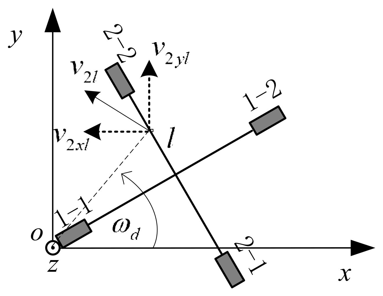
Similarly, 2-1 and 2-2 on the y-axis and thestate at moment $t$ are shown in Figure 3. Therefore, it can be inferred that the linear velocity near the junction point $l$ between the 1-2 end and the 1-1 and 1-2 electrodes is ${\mathit{v}}_{2l}={\omega }_d\sqrt{l^2+0.25\Delta l^2}$.

$$v_{2xl}=-{\omega }_d\sqrt{l^2+0.25\Delta l^2}\sin ({\omega }_{d}t)$$

(13)

$$v_{2yl}={\omega }_d\sqrt{l^2+0.25\Delta l^2}\cos ({\omega }_{d}t)$$

(14)

$$v_{2zl}=0$$

(15)

The three components of the electric field at $l$ for electrodes 2-1 and 2-2 can be obtained as follows:

$$E_{2xl}=v_{2yl}{B}_z-v_{2zl}{B}_y=B_z{\omega }_d\sqrt{l^2+0.25\Delta l^2}\cos ({\omega }_{d}t)$$

(16)

$$E_{2yl}=v_{2zl}{B}_x-v_{2xl}{B}_z=B_z{\omega }_d\sqrt{l^2+0.25\Delta l^2}\sin ({\omega }_{d}t)$$

(17)

$$E_{2zl}=v_{2xl}{B}_y-v_{2yl}{B}_x=-{\omega }_d\sqrt{l^2+0.25\Delta l^2}[B_y\sin ({\omega }_{d}t)+B_x\cos ({\omega }_{d}t)]$$

(18)

The measurement system shakes in the x-y plane, and the induced electric field on the 2-1 and 2-2 electrode pairs is

$$\begin{array}{l}{E}_{2d}={\displaystyle {\int }_{-\Delta l/2}^{\Delta l/2}[-E_{2xl}\sin ({\omega }_{d}t)+E_{2yl}\cos ({\omega }_{d}t)}]dl/\Delta l\\ \begin{array}{cc}& =\end{array}{\displaystyle {\int }_0^{\Delta l}0}dl/\Delta l=0\end{array}$$

(19)

Similarly, 3-1 and 3-2 are on the z-axis, and since the electrode pairs of 3-1 and 3-2 are perpendicular to the x-y plane, the linear velocity at any point between 3-1 and 3-2 is ${\mathit{v}}_{3l}=\frac{1}{2}{\omega }_d\Delta l$.

$$v_{3xl}=-\frac{1}{2}{\omega }_d\Delta l\sin ({\omega }_{d}t)$$

(20)

$$v_{3yl}=\frac{1}{2}{\omega }_d\Delta l\cos ({\omega }_{d}t)$$

(21)

$$v_{3zl}=0$$

(22)

Thus, the induced electric field on the 3-1 and 3-2 electrode pairs when the measurement system is swaying in the x-y plane is

$$E_{3xl}=v_{3yl}{B}_z-v_{3zl}{B}_y=\frac{1}{2}{B}_z{\omega }_d\Delta l\cos ({\omega }_{d}t)$$

(23)

$$E_{3yl}=v_{3zl}{B}_x-v_{3xl}{B}_z=\frac{1}{2}{B}_z{\omega }_d\Delta l\sin ({\omega }_{d}t)$$

(24)

$$E_{3zl}=v_{3xl}{B}_y-v_{3yl}{B}_x=-\frac{1}{2}{\omega }_d\Delta l[B_y\sin ({\omega }_{d}t)+B_x\cos ({\omega }_{d}t)]$$

(25)

Therefore, the induced electric field on the 3-1 and 3-2 electrode pairs when the measurement system is shaking in the x-y plane is

$$\begin{array}{l}{E}_{3d}={\displaystyle {\int }_0^{\Delta l}{E}_{3zl}}dl/\Delta l\\ \begin{array}{cc}& =\end{array}{\displaystyle {\int }_0^{\Delta l}-\frac{1}{2}{\omega }_d\Delta l[B_y\sin ({\omega }_{d}t)+B_x\cos ({\omega }_{d}t)]}dl/\Delta l\\ \begin{array}{cc}& =\end{array}-\frac{1}{2}{\omega }_d\Delta l[B_y\sin ({\omega }_{d}t)+B_x\cos ({\omega }_{d}t)]\end{array}$$

(26)

2.2. The Measurement System Shakes in the x-z Plane

Similarly, the measurement system wobbles in the x-z plane, again with the 1-1 sensor at the origin of the coordinates, at time $t$, the velocity at point $l$ between electrodes 1-1 and 1-2 is ${\mathit{v}}_{1l}={\omega }_{p}l$, and its three components are represented as:

$$v_{1xl}=-{\omega }_{p}l\sin ({\omega }_{p}t)$$

(27)

$$v_{1yl}=0$$

(28)

$$v_{1zl}={\omega }_{p}l\cos ({\omega }_{p}t)$$

(29)

The three components of the electric field at $l$ for electrodes 1-1 and 1-2 can be obtained as

$$E_{1xl}=v_{1yl}{B}_z-v_{1zl}{B}_y=-B_y{\omega }_{p}l\cos ({\omega }_{p}t)$$

(30)

$$E_{1yl}=v_{1zl}{B}_x-v_{1xl}{B}_z={\omega }_{p}l[B_x\cos ({\omega }_{p}t)+B_z\sin ({\omega }_{p}t)]$$

(31)

$$E_{1zl}=v_{1xl}{B}_y-v_{1yl}{B}_x=-B_y{\omega }_{p}l\sin ({\omega }_{p}t)]$$

(32)

Thus, the induced electric field on the electrode pair 1-1 and 1-2 is

$$\begin{array}{l}{E}_{1p}={\displaystyle {\int }_0^{\Delta l}[E_{1xl}\cos ({\omega }_{p}t)+E_{1zl}\sin ({\omega }_{p}t)}]dl/\Delta l\\ \begin{array}{cc}& =\end{array}{\displaystyle {\int }_0^{\Delta l}-B_y{\omega }_{p}l}dl/\Delta l=-\frac{1}{2}{B}_y{\omega }_p\Delta l\end{array}$$

(33)

Similarly, the linear velocity used at any point $l$ between 2-1 and 2-2 in the y-axis direction is ${\mathit{v}}_{2l}=\frac{1}{2}{\omega }_p\Delta l$. The three components of the electric field at $l$ on electrodes 2-1 and 2-2 can be obtained as follows:

$$E_{2xl}=v_{2yl}{B}_z-v_{2zl}{B}_y=-\frac{1}{2}{B}_y{\omega }_p\Delta l\cos ({\omega }_{p}t)$$

(34)

$$E_{2yl}=v_{2zl}{B}_x-v_{2xl}{B}_z=\frac{1}{2}{\omega }_p\Delta l[B_x\cos ({\omega }_{p}t)+B_z\sin ({\omega }_{p}t)]$$

(35)

$$E_{2zl}=v_{2xl}{B}_y-v_{2yl}{B}_x=-\frac{1}{2}{B}_y{\omega }_p\Delta l\sin ({\omega }_{p}t)]$$

(36)

Therefore, when the measurement system shakes in the x-z plane, the induced electric field on the 2-1 and 2-2 electrode pairs is as follows:

$$\begin{array}{l}{E}_{2p}={\displaystyle {\int }_0^{\Delta l}{E}_{2yl}}dl/\Delta l\\ \begin{array}{cc}& =\end{array}{\displaystyle {\int }_0^{\Delta l}\frac{1}{2}{\omega }_p\Delta l[B_x\cos ({\omega }_{p}t)+B_z\sin ({\omega }_{p}t)]}dl/\Delta l\\ \begin{array}{cc}& =\end{array}\frac{1}{2}{\omega }_p\Delta l[B_x\cos ({\omega }_{p}t)+B_z\sin ({\omega }_{p}t)]\end{array}$$

(37)

The electrode pairs 3-1 and 3-2 are on the z-axis, and the linear velocity near the connection point between the 3-2 end and the 1-1 and 1-2 electrodes is ${\mathit{v}}_{3l}={\omega }_p\sqrt{l^2+0.25\Delta l^2}$.

The three components of the electric field at l for electrodes 3-1 and 3-2 can be obtained as follows:

$$E_{3xl}=v_{3yl}{B}_z-v_{3zl}{B}_y=-B_y{\omega }_p\sqrt{l^2+0.25\Delta l^2}\cos ({\omega }_{p}t)$$

(38)

$$E_{3yl}=v_{3zl}{B}_x-v_{3xl}{B}_z={\omega }_p\sqrt{l^2+0.25\Delta l^2}[B_x\cos ({\omega }_{p}t)+B_z\sin ({\omega }_{p}t)]$$

(39)

$$E_{3zl}=v_{3xl}{B}_y-v_{3yl}{B}_x=-B_y{\omega }_p\sqrt{l^2+0.25\Delta l^2}\sin ({\omega }_{p}t)]$$

(40)

Therefore, the induced electric field on the 3-1 and 3-2 electrode pairs when the measurement system is shaking in the x-z plane is as follows:

$$\begin{array}{l}{E}_{3p}={\displaystyle {\int }_{-\Delta l/2}^{\Delta l/2}[-E_{3xl}\sin ({\omega }_{d}t)+E_{3\mathrm{z}l}\cos ({\omega }_{d}t)}]dl/\Delta l\\ \begin{array}{cc}& =\end{array}{\displaystyle {\int }_0^{\Delta l}0}dl/\Delta l=0\end{array}$$

(41)

2.3. The Measurement System Shakes in the y-z Plane

The metal navigation body measurement system shakes in the y-z plane, with the 1-1 sensor located at the coordinate origin, which is equivalent to the measurement system rotating around the 1-1 and 1-2 electrode pairs. The linear velocity of the 1-1 and 1-2 electrode pairs is zero, so the generated t interference-induced electric field is also zero, that is,

$$E_{1r}=0$$

(42)

The 2-1 and 2-2 electrode pairs and the 3-1 and 3-2 electrode pairs are shaking around their midpoints in the y-z plane, respectively. Taking 2-1 and 2-2 electrode pairs as research objects, the distance from the center point of the system is $l$, and it is close to electrodes 2-2, where the speed is ${\mathit{v}}_{2l}={\omega }_{r}l$.

The three components of the velocity can be found to be the following:

$$v_{2xl}=0$$

(43)

$$v_{2yl}=-{\omega }_{r}l\sin ({\omega }_{r}t)$$

(44)

$$v_{2zl}={\omega }_{r}l\cos ({\omega }_{r}t)$$

(45)

The three components of the electric field at $l$ for electrodes 2-1 and 2-2 can be obtained as follows:

$$E_{2xl}=v_{2yl}{B}_z-v_{2zl}{B}_y=-{\omega }_{r}l[B_z\sin ({\omega }_{r}t)+B_y\cos ({\omega }_{r}t)]$$

(46)

$$E_{2yl}=v_{2zl}{B}_x-v_{2xl}{B}_z=B_x{\omega }_{r}l\cos ({\omega }_{r}t)$$

(47)

$$E_{2zl}=v_{2xl}{B}_y-v_{2yl}{B}_x=B_x{\omega }_{r}l\sin ({\omega }_{r}t)$$

(48)

Thus, the induced electric field on the 2-1 and 2-2 electrode pairs when the measurement system is swaying in the y-z plane is as follows:

$$\begin{array}{l}{E}_{2r}={\displaystyle {\int }_{-\Delta l/2}^{\Delta l/2}[E_{2yl}\cos ({\omega }_{d}t)+E_{2zl}\sin ({\omega }_{d}t)}]dl/\Delta l\\ \begin{array}{cc}& =\end{array}{\displaystyle {\int }_{-\Delta l/2}^{\Delta l/2}{B}_x{\omega }_{r}l}dl/\Delta l=0\end{array}$$

(49)

Similarly, the induced electric field on the 3-1 and 3-2 electrode pairs when the measurement system is shaking in the y-z plane is as follows:

$$E_{3r}=0$$

(50)

It can be obtained that the three components of the induced electric field output from the three-axis sensor when the measurement system is swaying at all three angles are as follows:

$$E_1=E_{1d}+E_{1p}+E_{1r}$$

(51)

$$E_2=E_{2d}+E_{2p}+E_{2r}$$

(52)

$$E_3=E_{3d}+E_{3p}+E_{3r}$$

(53)

Based on the above theoretical analysis, it can be concluded that the induced electric field output during the shaking of the three-axis measurement system is related to the center point of the shaking. The expression for the interference-induced electric field is obtained by shaking one sensor as the center point (always with the 1-1 electrode as the shaking center in Figure 1). By changing the shaking center, assuming that the shaking center is the center point of the measurement system (i.e., the intersection point of the three axes), the interference electric field output during the three-axis shaking is zero.

3. Analysis of the Characteristics of the Induce Electric Field in Metal Vehicle Motion

Based on the theoretical model in Section 2, it can be obtained that the interference electric field output in the case of uniform motion or shaking of the measurement system has the following characteristics:

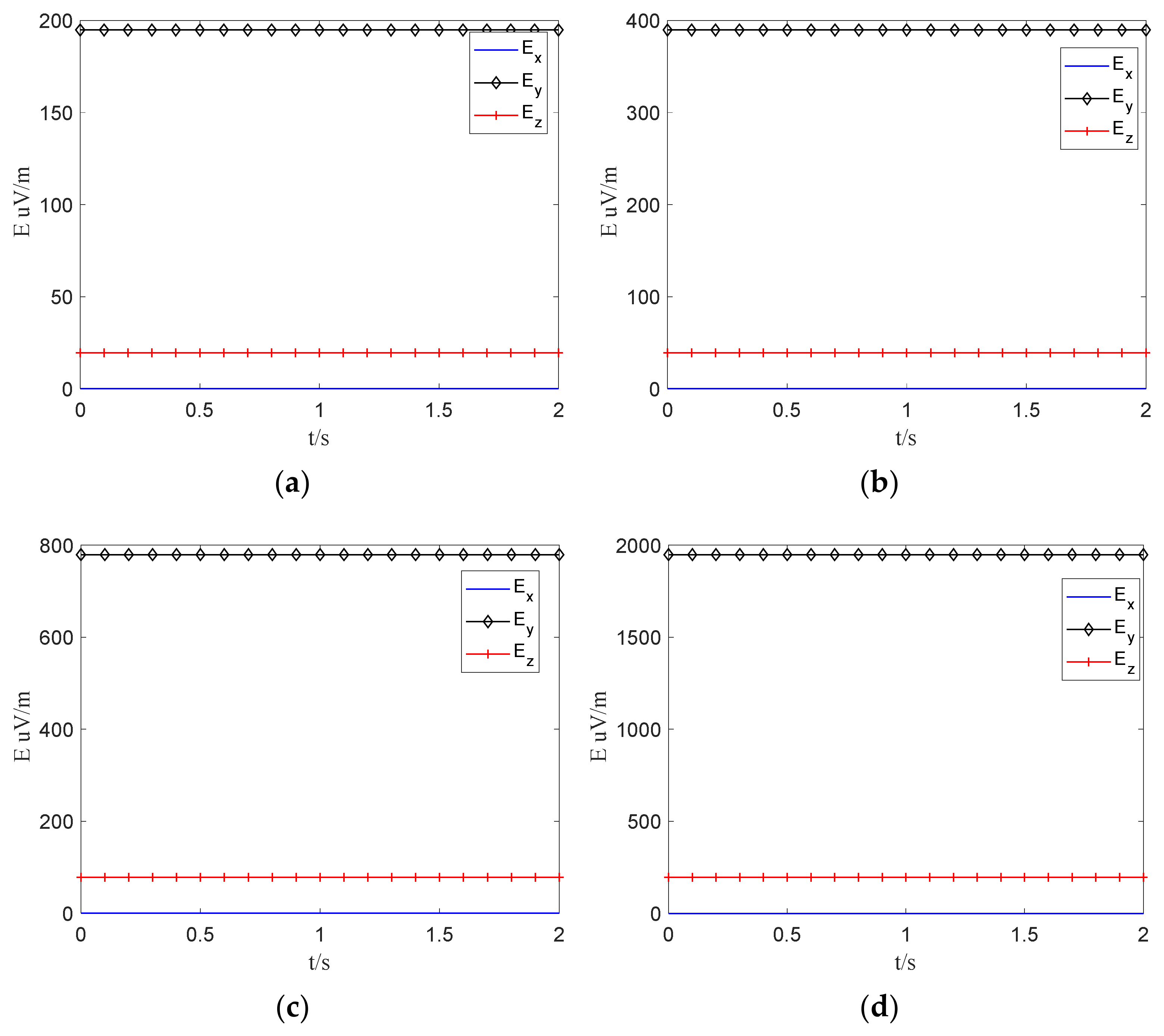
When moving at a constant speed, it can be seen from Equations (3)–(5) that the induced electric field interference output by the measurement system is a static signal. The magnitude of the static electric field is directly proportional to the speed of movement and the size of the geomagnetic field, and the magnitude of each component is related to the direction of movement and the size of the geomagnetic field component.

The three components of the induced electric field simulated by taking the geomagnetic field intensity $F=\mathrm{45,000}$ nT, magnetic inclination angle $I=\pi /3$, magnetic declination $\gamma =\pi /18$, and motion speed $\mathit{v}=(5,0,0)$, $\mathit{v}=(10,0,0)$, $\mathit{v}=(20,0,0)$ and $\mathit{v}=(50,0,0)$, respectively, are shown in the figure below. According to Figure 4, the induced electric field at this speed is a static electric field, and its magnitude will change with the change in speed and geomagnetic field in the navigation area. When the speed reaches 50 m/s, the magnitude can reach 2 mV/m.

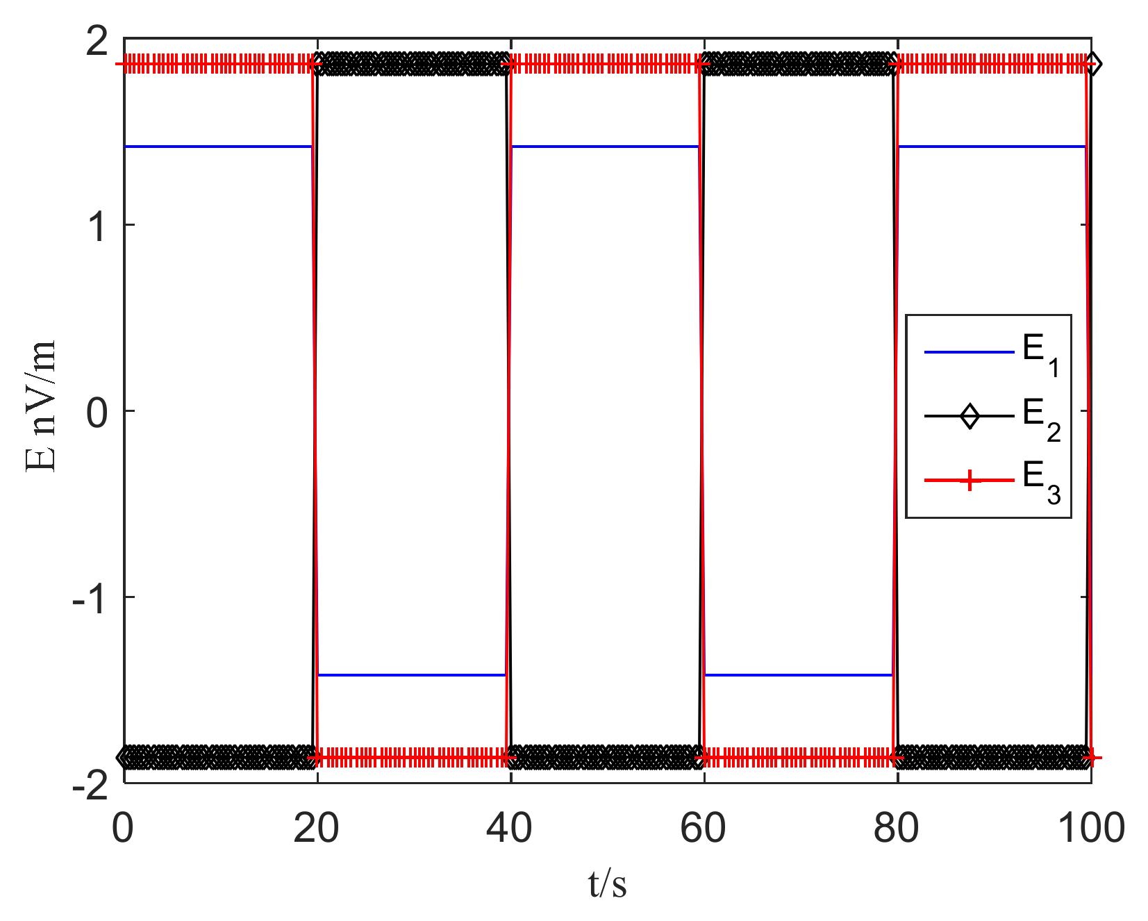
Taking the geomagnetic field intensity $F=\mathrm{45,000}$ nT, the magnetic inclination angle $I=\pi /3$, and the magnetic declination angle $\gamma =\pi /18$ and considering the actual situation, the maximum angle of shaking of the high-speed projectile after stability is about 0.1°, and the shaking speed is 0.005°/s [18]. The shaking speed and angle of pitch, roll, and heading are consistent. When the shaking angle of the navigation body is 0.1°, the simulation results of the induced electric field are shown in Figure 5, itcan be seen from Figure 5 that the interference caused by the high-speed projectile shaking is in the nV/m range and the frequency is extremely low. At this shaking intensity, it will not affect the detection of motion targets.

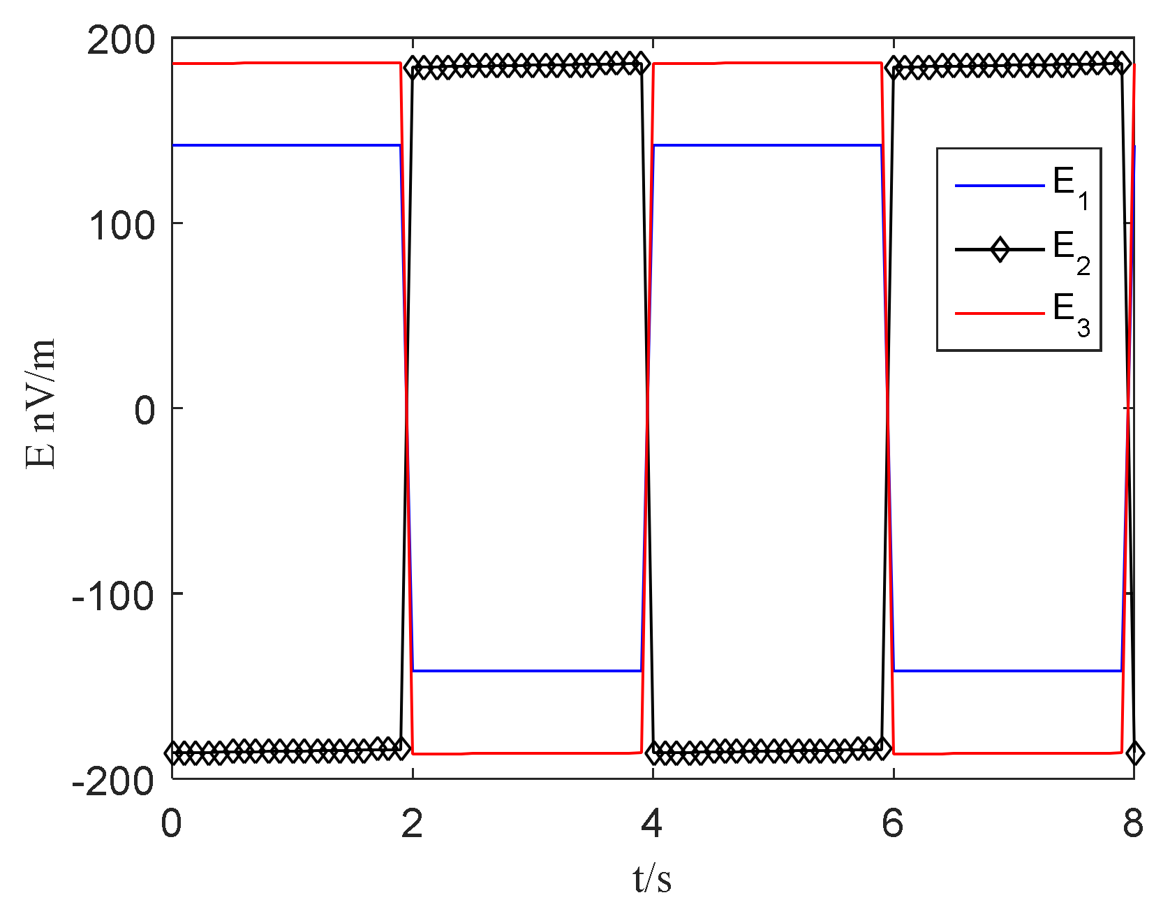
Assuming in the ultimate shaking state [20], where the shaking speed is 0.5°/s and the maximum angle is still 1°, and the simulation results are shown in Figure 6. From the figure, it can be seen that the maximum peak-to-peak noise caused by the shaking of the high-speed aircraft is about 180 nV/m, and the frequency is related to the shaking angular velocity and amplitude. At this shaking intensity, it still does not affect the detection of the vehicle target.

4. Maritime Verification Experiment

An at-sea measurement study was carried out to verify the electric field interference characteristics of platforms shaken by metallic vehicles and to provide a basis for the study of electric field detection methods on moving platforms.

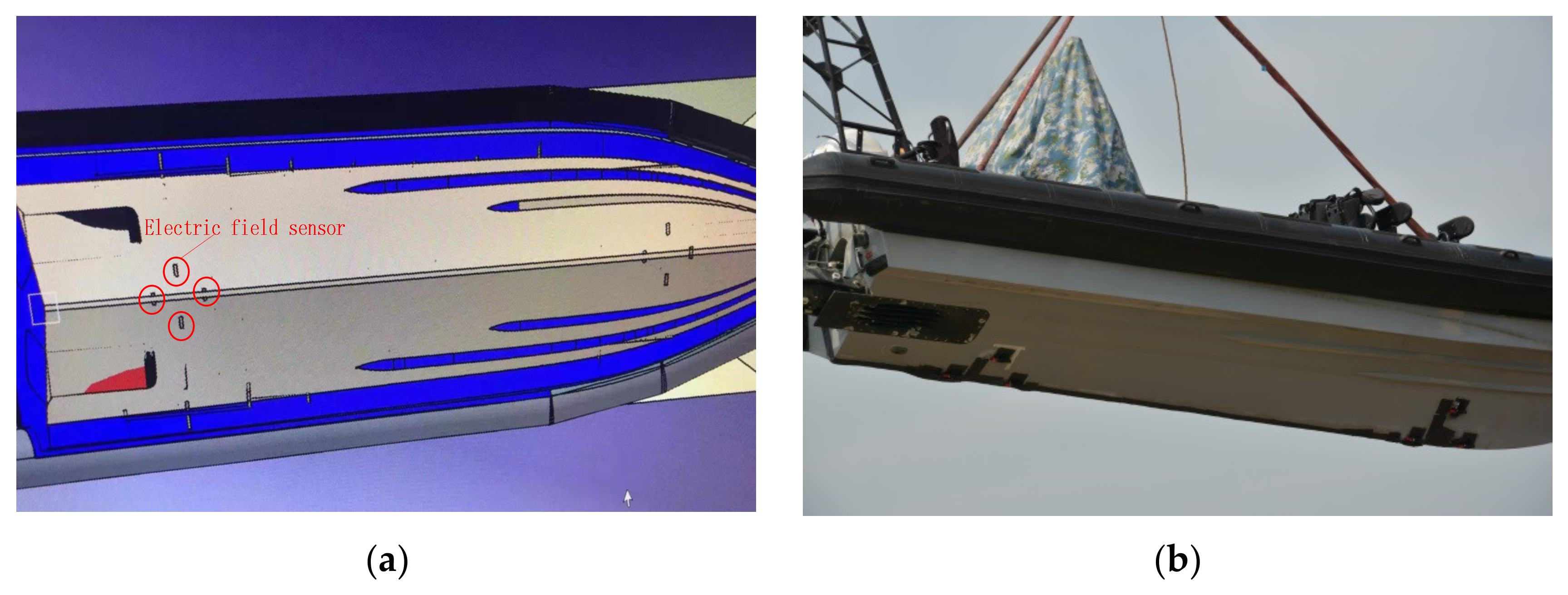
The experiment uses a high-speed speedboat as a metal navigation body platform; its propulsion system adopts pump-jet propulsion, and the highest speed can reach more than 50 knots; the electric field sensor consists of four Ag/AgCl electrodes, used to measure along the direction of the speedboat and the speedboat transverse direction of the two horizontal components of the electric field; the installation schematic diagram, as shown in Figure 7a, shows two measurements in each direction of the electric field. The electrode distance of the sensor is 0.5 m, and at the same time, in order to reduce the impact of the sensor’s connecting wire shaking, the sensor and the wire are fixed on the surface of the hull using a strong adhesive and clamps, and the wire is outside the parcel layer, which not only ensures that the sensor and wire in the movement process itself do not produce shaking (only with the hull of the ship shaking) but also ensures that the sensor and the wire do not fall off during the high-speed movement of the speedboat. The installation on the real boat is shown in Figure 7b.

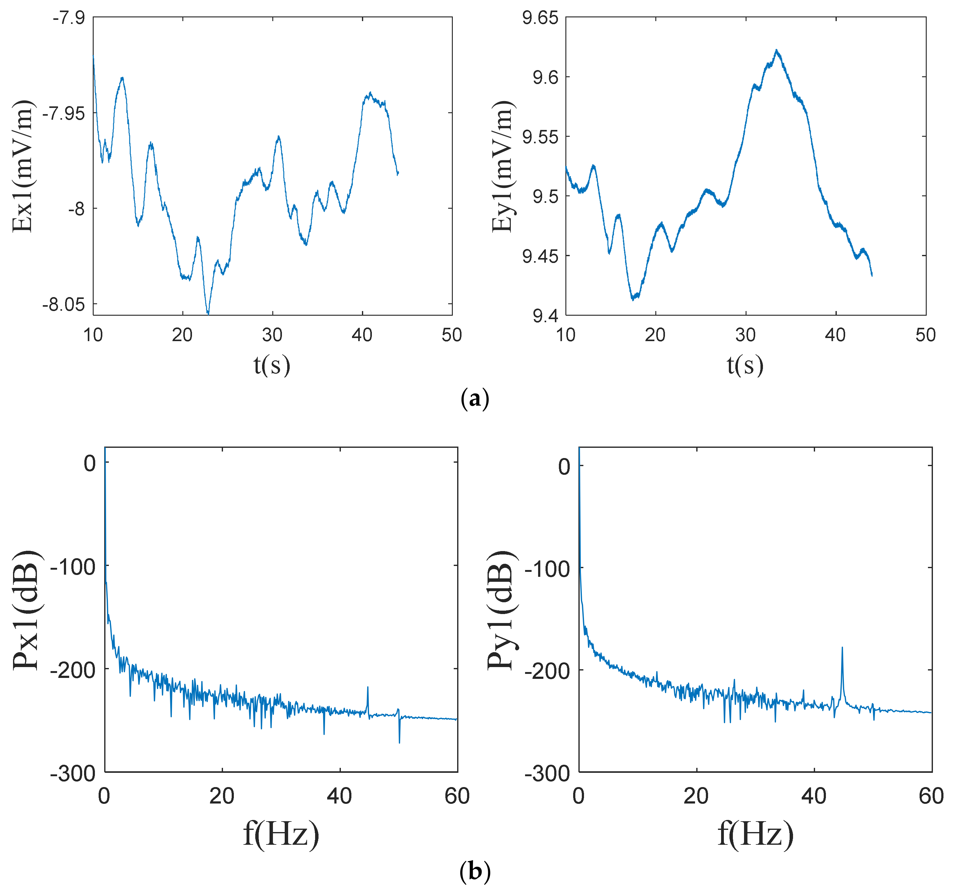
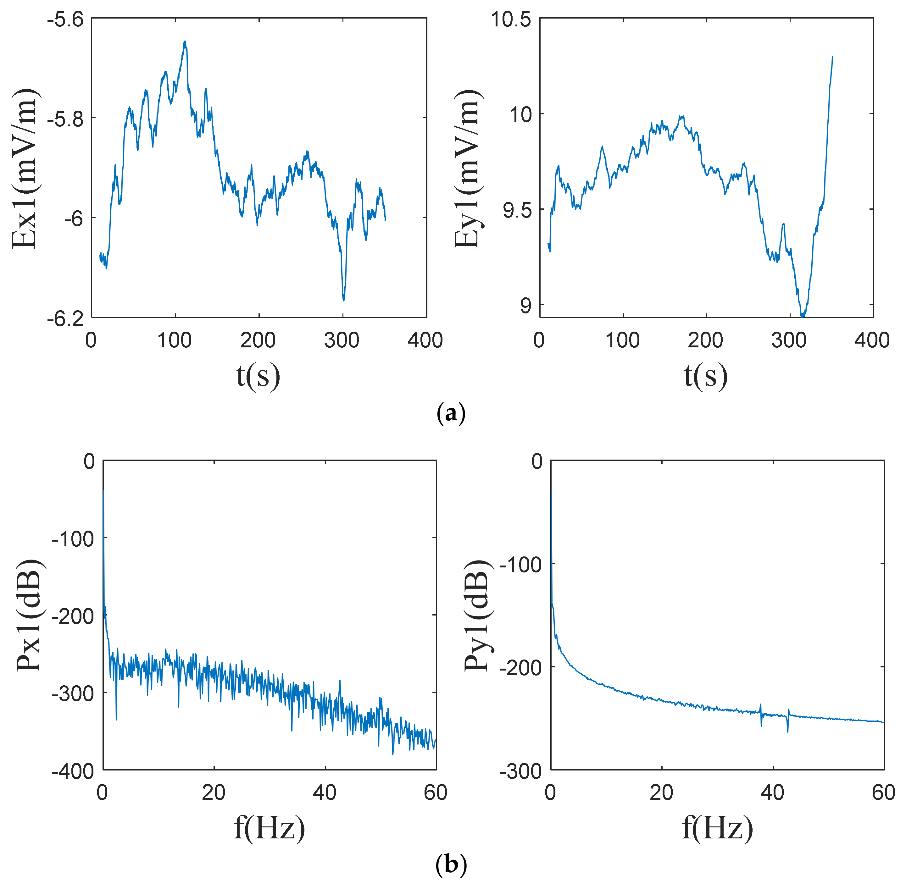
The water depth of the experimental sea area is about 5 m, and the conductivity of seawater is measured to be 2.8 S/m. The forward direction of the speedboat is defined to be in the x-axis direction, and the sampling rate of the system is 250 Hz. Figure 8 shows the background electric field of the platform of the speedboat with the engine turned off, and the surface of the sea is in a state of free swaying.

As can be seen from Figure 8 and Figure 9, when the speedboat platform floats on the sea surface, the total electric field signal can reach the order of mV/m, and most of its energy is concentrated in the low-frequency band, especially in the part of the frequency band below 1 Hz, which is close to the ship’s electrostatic field, so there is a larger probability of false alarms when using the ship’s electrostatic field to detect it; there is a stronger industrial frequency interference near 50 Hz, which belongs to high frequency in comparison with the ship’s low-frequency electric field. There is a strong industrial frequency interference near 50 Hz, which is a high frequency compared to the ship’s low-frequency electric field, and the ship’s axial frequency electric field signal can be detected in this background.

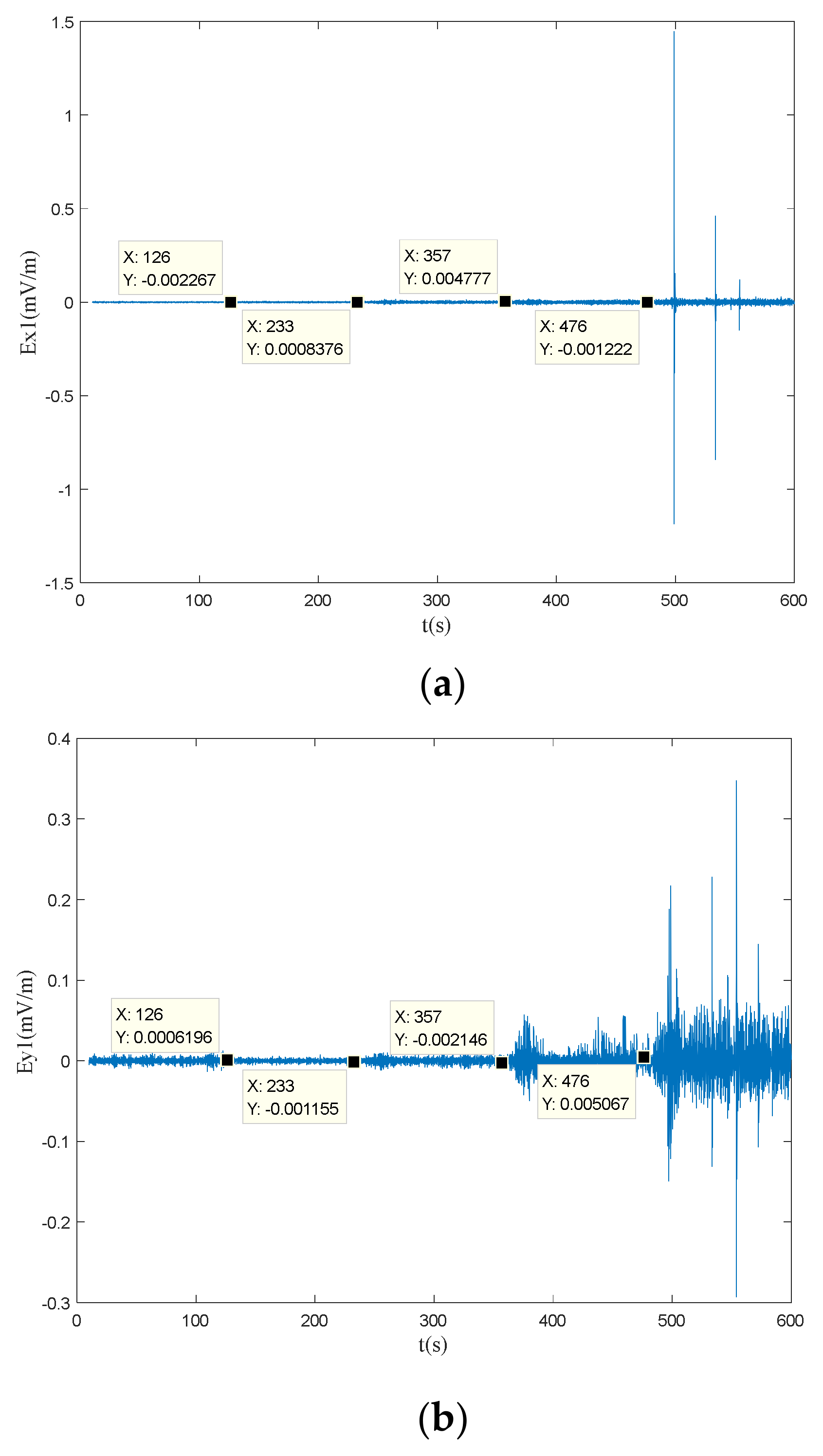
To verify the electric field interference characteristics of the measurement system under uniform motion state. Due to the fact that the propeller rotation frequency of ships at economic speeds is always higher than 1 Hz, which is 60 revolutions per minute, the interference analysis frequency band focuses on the 1–30 Hz; focus on the analysis of the background interference within the frequency band of the axial frequency electric field, the use of the speedboat platform to measure the background electric field interference under the motion speeds of 5, 10, and 20 knots, respectively, and the time domain signals are shown in Figure 10.

As shown in Figure 10, at 0–116 s, the speed is 5 knots; at 126–233 s, the speed is 10 knots; and at 357–476 s, the speed is 20 knots. As can be seen from the figure, along the speedboat sailing direction, the 1~30 Hz frequency band electric field component peak value in the boat speed is lower than 20 knots, relatively small; the electric field amplitude is less than 20 $\mathsf{\mu }\mathrm{V}/\mathrm{m}$ at speeds of 5 knots and 10 knots, andapproximately 30 $\mathsf{\mu }\mathrm{V}/\mathrm{m}$ at a speed of 20 knots; the amplitude of the interference electric field spectrum perpendicular to the navigation direction (y-direction) increases significantly with the increase in navigation speed, which is caused by the cutting of the geomagnetic field by the wire. The equivalent length of the geomagnetic field wire cut perpendicular to the navigation direction is longer, and it will increase significantly with the increase in navigation speed.

Calculated at 20 knots, the spectral density of the background interference electric field of the speedboat in the frequency band of 1~30 Hz is about 0.4 $\mathsf{\mu }\mathrm{V}/\sqrt{\mathrm{H}\mathrm{z}}$, which is still lower than most of the target electric fields of the ship, so it is possible to detect the electric field signals of the ship by using this speedboat with the electric field detection system on board.

5. Conclusions

In this paper, based on Faraday’s law of electromagnetic induction, combined with the electric field detection system, the induced electric field model of the motion of a metallic vehicle is deduced. The induced electric field generated by the underwater metallic vehicle shaking in different planes of x-y, x-z, and y-z is derived, and the three-component output model of the induced electric field output from the three-axis sensor is further derived by solving the induced electric field of the electrode pairs in the different planes when the measurement system is shaking at all three angles. Based on the above theoretical model, it can be seen that when moving at a uniform speed, the induced electric field interference output from the measurement system is a static signal, the size of the static electric field is proportional to the motion speed and the magnitude of the geomagnetic field, and the magnitude of each component is related to the direction of the motion and the magnitude of the component of the geomagnetic field, whereas the noise of the induced electric field generated by the pitching, rolling, and swaying changes in the direction of the vehicle under the stable state is of the order of nV/m, which will not have a great influence on the detection. The noise generated by the induced electric field in the case of pitching, rolling, and swaying is of the order of nV/m, which does not affect the detection. The correctness of the theoretical model is verified by using the speedboat platform in conjunction with the sea experiments. The spectral density of the background interference electric field of the speedboat in the frequency band of 1~30 Hz is about 0.4 $\mathsf{\mu }\mathrm{V}/\sqrt{\mathrm{H}\mathrm{z}}$ at 20 knots, which makes it feasible to detect the electric field of the ship by using the speedboat platform.

The models and conclusions obtained in this paper are of guiding significance for analyzing the induced electric field generated by the motion of underwater vehicles, especially high-speed navigational vehicles, and they also verify that it is feasible for underwater vehicles to be equipped with an electric field detection system. The next step will be to consider the use of underwater motion platforms to carry out real ship target detection experiments, and, at the same time, carry out research on platform signal processing methods.