MMDL-Net: Multi-Band Multi-Label Remote Sensing Image Classification Model

Abstract

High-resolution remote sensing imagery comprises spatial structure features of multispectral bands varying in scale, color, and shape. These heterogeneous geographical features introduce grave challenges to the fine segmentation required for classification applications in remote sensing imagery, where direct application of traditional image classification models fails to deliver optimal results. To overcome these challenges, a multispectral, multi-label model, MMDL-Net, has been developed. This model is integrated with the multi-label BigEarthNet dataset, primarily employed for land cover classification research in remote sensing imagery, with each image composed of 13 spectral bands and spatial resolutions of 10 m, 20 m, and 60 m. To effectively utilize the information across these bands, a multispectral stacking module has been introduced to concatenate this spectral information. To proficiently process three distinct large-scale remote sensing image datasets, a multi-label classification module has been incorporated for training and inference. To better learn and represent the intricate features within the images, a twin-number residual structure has been proposed. The results demonstrate that the MMDL-Net model achieves a top accuracy of 83.52% and an F1 score of 77.97%, surpassing other deep learning models and conventional methods, thereby exhibiting exceptional performance in the task of multispectral multi-label classification of remote sensing imagery.

1. Introduction

A prominent application of remote sensing (RS) imagery is land use and land cover (LULC) classification. Traditional classification methods often fail to fully exploit the geometric information in remote sensing images, although texture features are sometimes utilized to supplement the spectral characteristics of such images [1]. There are a plethora of approaches to analyzing remote sensing images, including machine learning-based methods [2,3], such as Support Vector Machines (SVMs) [4] and Random Forests (RFs) [5], as well as deep learning methods like Convolutional Neural Networks (CNNs) and Deep Neural Networks (DNNs).

Remote sensing images are rich in information, necessitating classification methods that are both efficient and yield precise results. The advent of deep learning has effectively addressed this issue. The use of deep learning for the analysis of remote sensing images is becoming increasingly widespread across various research fields, such as perimeter mapping, ecosystem services [6,7], delineation of agricultural fields [8], large-scale mapping of tree crops [9], extensive road extraction [10], and detection of burned areas [11] Deep learning has also demonstrated high performance in classifying and extracting the necessary information from remote sensing images, as evidenced by achievements with network models like U-Net [12], Residual Networks (ResNet) [13], Deep Residual U-Net (ResU-Net) [14], convolutional network-based semantic segmentation [15], and Pyramid Scene Parsing Network (MP-Net) [16].

Existing image datasets are predominantly composed of three-channel RGB images formulated for computer vision tasks with single-label categorization. Standard CNN architectures are primarily tailored for processing these RGB images and lack the capability to effectively exploit the complex interrelationships among multispectral channels. When applied to remote sensing imagery, these models exhibit deficiencies, including but not limited to inadequate handling of the inherent high-dimensional characteristics of hyperspectral images and challenges in addressing the spectral and spatial correlations within these images. Consequently, conventional CNNs are insufficient for remote sensing tasks. Sumbul provided a multi-label, multi-resolution dataset named BigEarthNet, comprising 590,326 images, each annotated with multiple labels from the CORINE Land Cover database [17]. In the context of LULC scene classification tasks, Mañas et al. demonstrated that models pre-trained with contrastive learning on BigEarthNet outperformed those pre-trained on ImageNet [18]. Sumbul et al. proposed a triplet sampling strategy utilizing BigEarthNet data for learning high-quality feature representations for content retrieval [19]. Stojnic and Risojevic employed contrastive multiview coding for self-supervised pre-training [20]. Vincenzi et al. introduced a self-supervised learning method for satellite imagery, utilizing BigEarthNet labels for LULC scene classification, achieving significant results with their initialization approach [21].

In the application of remote sensing classification, Convolutional Neural Networks (CNNs) possess powerful feature extraction and model generalization capabilities, rapidly advancing in the field of computer vision, with a plethora of CNN-based models being employed for remote sensing image classification. Diakogiannis et al. presented a novel framework composed of a deep learning architecture, ResUNet-a, coupled with a new loss function based on the Dice coefficient, which achieved remarkable convergence characteristics [22]. However, the model may encounter blurring or incorrect segmentation in complex scenes. Kim et al. explored methods for quantifying the bias in DNNs for land usage, implementing DNN-based models through fine-tuning existing pre-trained models for school building recognition [23], but the accuracy and bias analysis results might not generalize to other regions or countries. Sumbul and Demir utilized a multi-attention strategy employing bidirectional long short-term memory networks to capture and leverage the spectral and spatial information content of RS images [24], employing complex multi-branch CNNs and multi-attention mechanisms, which resulted in high computational complexity. Koßmann et al. proposed an oversampling approach to address the issue of class imbalance in BigEarthNet’s land use/cover categories [25], but an excessive focus on minority classes could lead the model to perform well on these while underperforming in other classes. Dixit et al. used the Dilated-ResUnet deep learning architecture for extracting buildings and small objects [26], with the proposed model performing well on the FCC (NIR, Red, Green) dataset, but its performance may decrease on other spectral band combinations.

Among a plethora of models, we have discerned that the residual learning framework introduced by ResNet facilitates the simplification of training processes for otherwise challenging deep networks. Furthermore, the deep structure of ResNet is capable of learning a broad spectrum of features ranging from generic to specific, which proves to be extremely beneficial for classifying the diverse categories present within remote sensing data. The block structure of ResNet also permits easy modifications and expansions of the network to meet the specific requirements of the task at hand. Mobeen ur Rehman et al. have proposed a deep architecture endowed with a Region Proposal Network (RPN) that exploits the texture and edges of images to extract pertinent regions by sliding a network over feature maps extracted from deep architectures, namely VGGNet and ResNet, where the deep capabilities of ResNet have exhibited commendable performance [27]. Long Wen et al. have introduced a novel 51-layer TCNN (ResNet-50) for fault diagnosis, which utilizes the ResNet-50, trained on ImageNet, as a feature extractor for fault diagnosis, outperforming other deep learning models and traditional methods, thus reaffirming the transfer learning capabilities of ResNet [28]. Devvi Sarwinda et al. have put forth an image classification methodology based on the ResNet architecture for the detection of colorectal cancer, demonstrating favorable classification performance. ResNet has also produced highly reliable and reproducible results in biomedical image analysis [29]. Tao Zhou et al. have proposed a COVID-ResNet auxiliary diagnostic model based on CT images, where the squeeze-and-excitation mechanism of ResNet’s residual connections, coupled with the easily modifiable and expandable block structure of ResNet, has resulted in enhanced performance [30]. Swalpa Kumar Roy et al. have introduced an attention-based adaptive spectral-spatial kernel improved residual network (A2S2K-ResNet), incorporating an attention mechanism and refining the residual modules of ResNet with three-dimensional ResBlocks to jointly extract spectral-spatial features, yielding impressive classification outcomes [31]. The feature fusion capability of the ResNet model, which integrates layers or modules that combine spatial and spectral features, along with its customized classification head, exhibits clear advantages in the design of multi-label classification.

To address the complex task of classifying remote sensing imagery applications, this paper introduces MMDL-Net, a multispectral, multi-label classification model designed for high-resolution remote sensing imagery. It incorporates a multispectral stacking module, a multi-label classification module, and a feature extraction module that combines Residual Networks (ResNets) with TensorFlow. This module captures global information as base-level features from feature maps, and by increasing the number of channels, it ensures the transfer of more detailed information, providing an expanded feature representation space. The network’s input layer and fully connected layer are further designed to enhance the network’s robustness to changes and noise in the input images, thereby improving classification accuracy. A multi-label classification sigmoid function is designed to independently output a probability for each category, with each category’s output being independent, making it highly suitable for multi-label classification tasks.

The paper makes significant contributions in the following areas:

• Through meticulous analysis and comparison of existing remote sensing image classification methods, it adopts a multispectral multi-label classification strategy to efficiently extract features from high-resolution remote sensing images;
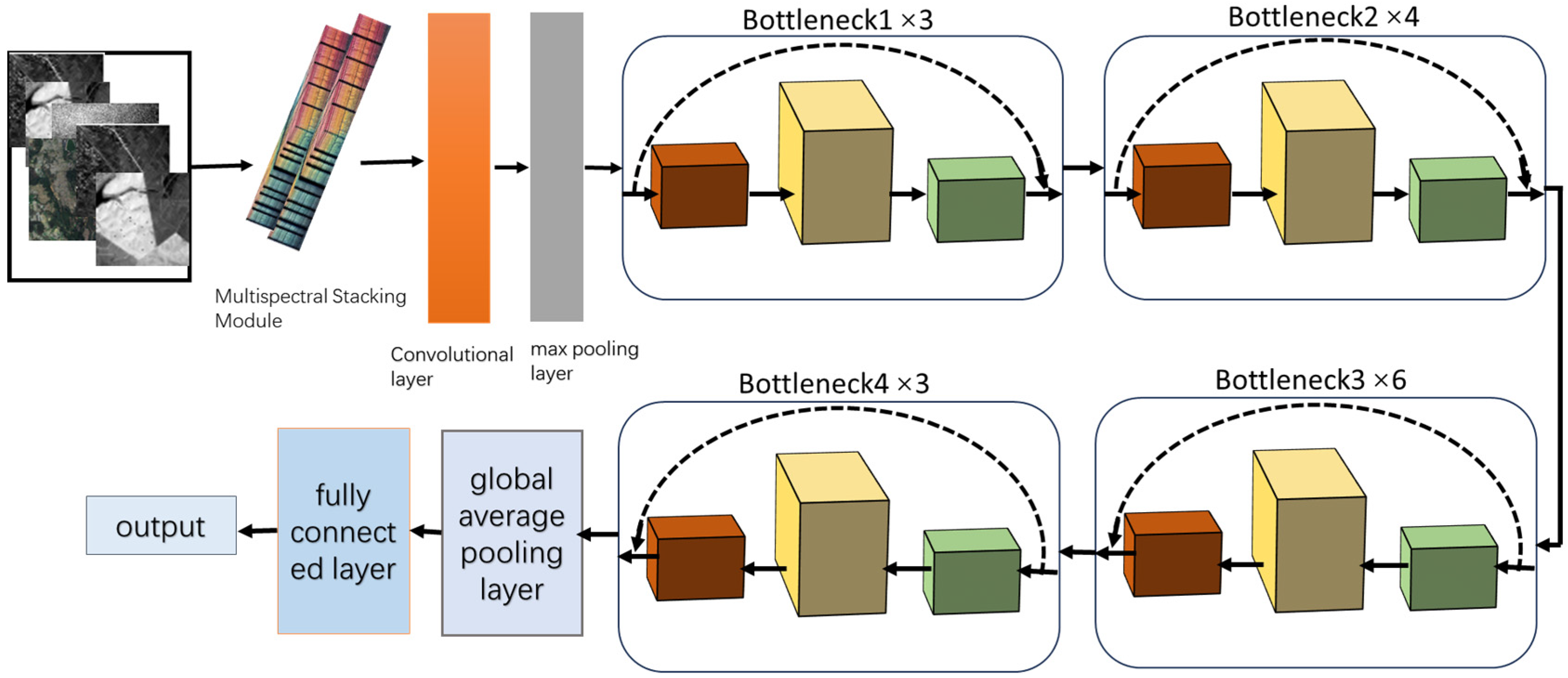
• It proposes a novel dual-number residual structure and multi-label classification module that can better learn and capture the details and semantic information of the input images, enabling the network to better adapt to the complex task of classifying remote sensing imagery applications;
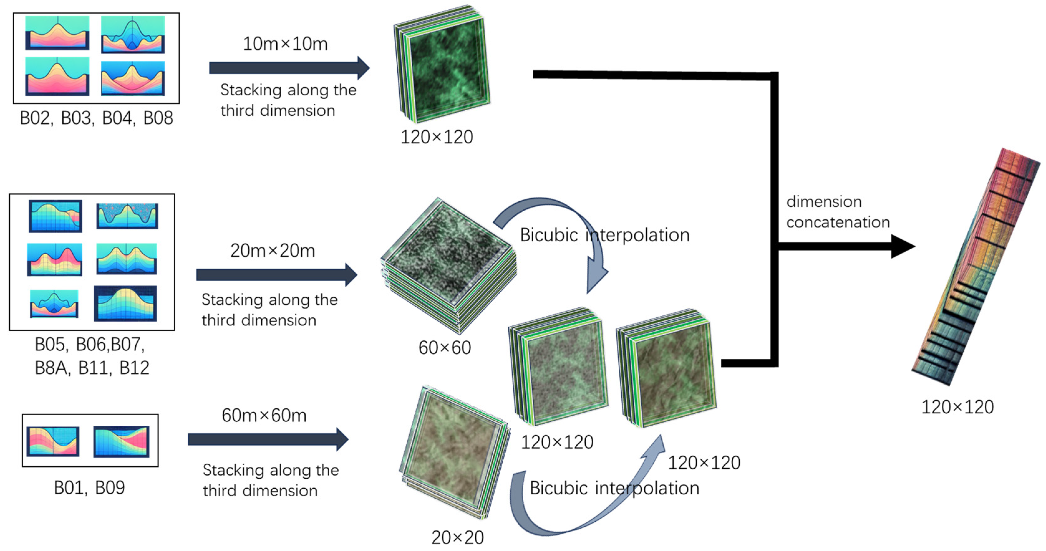
• It introduces a multispectral stacking module that effectively integrates information from bands of varying resolutions, thereby enriching the surface information available.

Based on these contributions, the paper presents MMDL-Net, a powerful model aimed at effectively solving the task of application classification for high-resolution remote sensing imagery.

The organization of the work is as follows: Section 2 provides an overview of the structure of the MMDL-Net model and introduces the MMDL-Net model along with all its internal components. Section 3 describes the experimental setup and the analysis of results. Discussions are presented in Section 4. Conclusions are drawn in Section 5.

2. Materials and Methods

In recent years, the continuous enhancement in the spatial resolution of remote sensing images has encapsulated more complex features, significantly raising the bar for image feature extraction. Considering the prowess of the ResNet architecture in deep feature extraction, multiscale processing, and overcoming spectral limitations, this work adopts it as the foundational framework. It integrates a multispectral stacking module and a multi-label classification module, with optimizations conducted from four perspectives: the residual blocks, input and output layers, fully connected layers, and loss functions. During the feature extraction phase, to better learn and represent the intricate features in remote sensing imagery, this paper doubles the number of channels within each residual block and adjusts the threshold to prevent overfitting. To achieve enhanced classification performance, the pixel size of the input layer is modified to 120 × 120 to align with the dataset, while the output layer is linked with the fully connected layer, utilizing 19 classes. For an appropriate loss function within multi-label multi-classification tasks, the binary cross-entropy loss function is employed in the TensorFlow design. This choice facilitates easier gradient computation without the need for any encoding transformations of the labels.

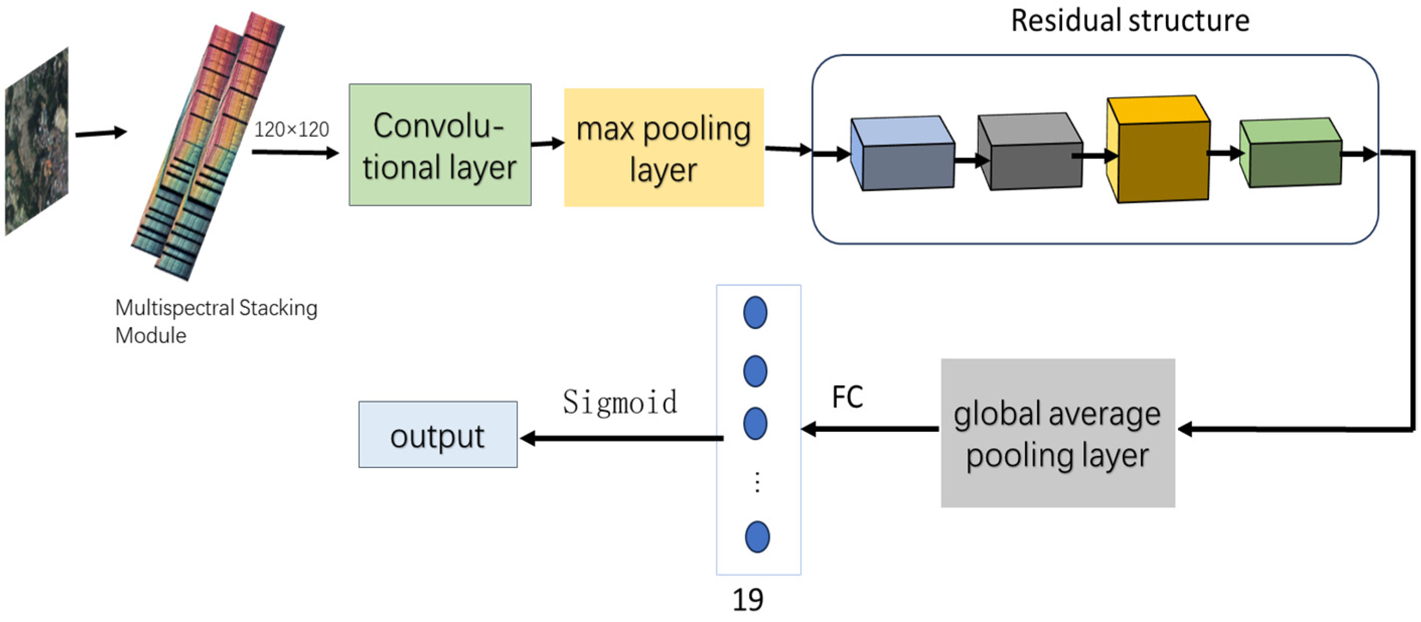
2.1. Multispectral Stacking Module

The BigEarthNet remote sensing image repository is sourced from the Sentinel-2 satellite, which is equipped with 13 multispectral bands and is a product of the European Space Agency (ESA), headquartered in Paris, France. It provides diverse typologies of Earth’s surface information. These bands span the spectral regions of visible light, near-infrared, and shortwave infrared, a design that confers an advantage in applications such as monitoring vegetation health, agricultural management, forest surveillance, and land cover change detection. In contrast, other common satellites like Landsat or MODIS may be more suitable for long-term time series analysis, atmospheric and oceanic studies, as well as broad-scale global dynamic monitoring. The primary uses of each band and the types of information they typically represent are shown in

Table 1. Information represented by the 13 bands and their primary uses.

Band Number	Central Wavelength (nm)	Primary Use
B01	443	Coastal aerosol detection and atmospheric conditions
B02	490	Blue band–Vegetation, soil, and water bodies
B03	560	Green band–Vegetation health and vitality
B04	665	Red band–Chlorophyll content for plant health
B05	705	Red edge–Vegetation characteristics and biomass
B06	740	Red edge–Vegetation characteristics and biomass
B07	783	Red edge–Vegetation characteristics and biomass
B08	842	NIR–Plant health and biomass estimation
B8A	865	Narrow NIR–Improved vegetation health assessment
B09	940	Water vapor estimation
B10	1375	Cirrus cloud detection
B11	1610	SWIR–Moisture content, vegetation stress
B12	2190	SWIR–Mineral content, soil properties, heat detection

.

The multispectral stacking module is positioned before the input module of the model, leveraging information from 12 distinct spectral bands while excluding the 10th band, which does not reflect surface information. In contrast to conventional RGB images, which comprise only three bands—where the R (red) channel corresponds to the B04 band, the G (green) channel corresponds to the B03 band, and the B (blue) channel corresponds to the B02 band—this module aims to effectively integrate information from a larger number of bands. To accommodate the varying resolutions of satellite image data, the 12 bands are divided into three groups.

The four bands with a resolution of 10 m (B02, B03, B04, B08), each with dimensions of 120 × 120, are stacked along the third dimension to create a new tensor, thereby generating an image with four channels. Similarly, the six bands with a resolution of 20 m (B05, B06, B07, B8A, B11, B12), each sized at 60 × 60, are stacked along the third dimension to form a new tensor, resulting in an image with six channels. The remaining two bands with a resolution of 60 m (B01, B09), each sized at 20 × 20, are also stacked along the third dimension to produce an image with two channels. Subsequently, images of bands with 20 m and 60 m resolutions are resized to match the 120 × 120 dimensions of the 10-m bands using bicubic interpolation. Finally, the module concatenates these three tensors along the third dimension, generating a new tensor that yields a multi-channel image of size 120 × 120. The structure of the multispectral stacking module is illustrated in Figure 1.

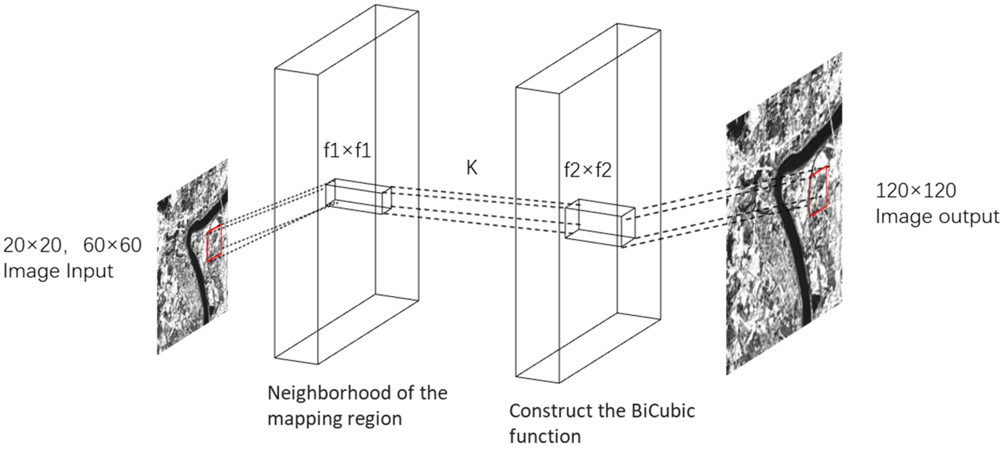
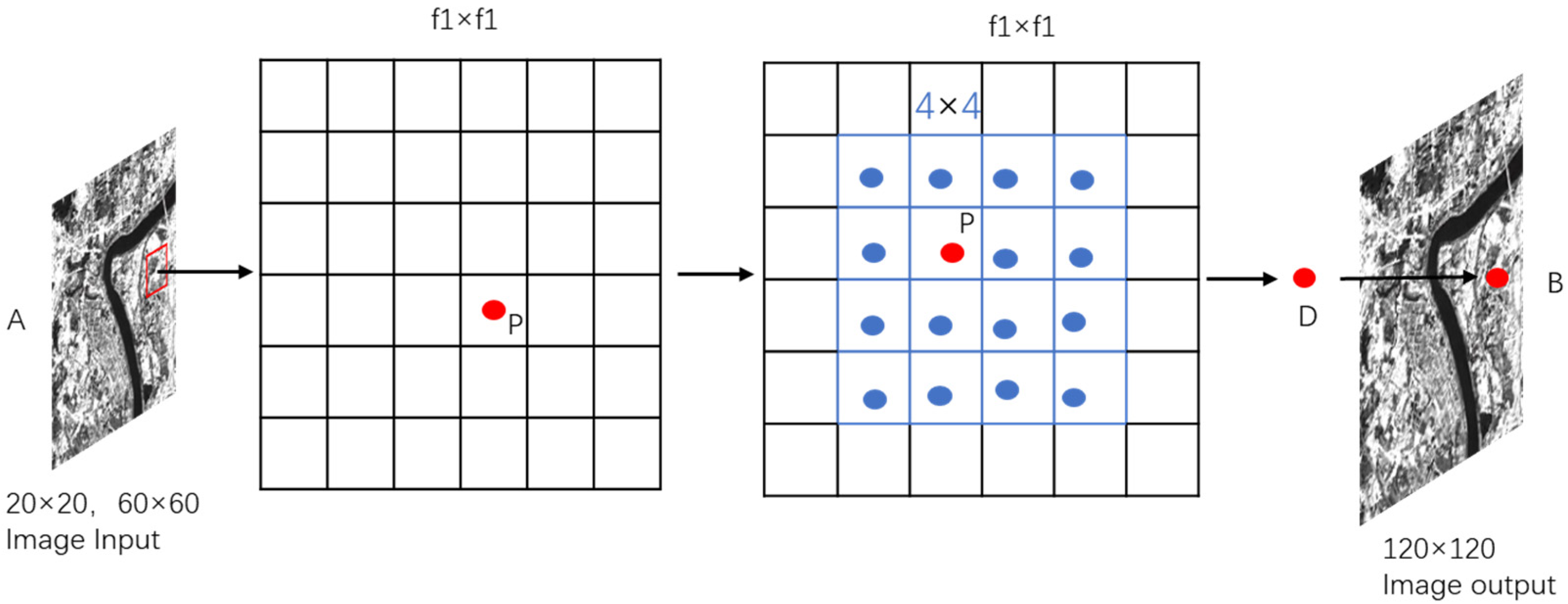
2.2. Model Input Adaptation and Interpolation in MMDL-Net

In order to accommodate the varying pixel sizes of remote sensing images in the BigEarthNet dataset, ranging from 20 × 20, 60 × 60, to 120 × 120, we enhanced the input layer of the ResNet network by adjusting the commonly used standard 224 × 224 size of RGB images to the maximum size within the dataset, which is 120 × 120. This modification aims to reduce computational demands, enhance efficiency, and better capture the details and features present in the images.

For images with dimensions smaller than 120 × 120 pixels, specifically those measuring 20 × 20 and 60 × 60 pixels, bicubic interpolation is implemented. In the context of multispectral remote sensing imagery, bicubic interpolation provides smoother transitions at edges compared to nearest-neighbor and bilinear interpolation techniques, thereby maintaining greater detail and image sharpness upon enlargement. This is particularly critical for the analysis of remote sensing images as it aids in preserving the delineation and intricate features of land objects, contributing to enhanced classification and recognition of these features. Accurate color interpolation is essential when processing multispectral remote sensing images due to its relation to the identification of spectral characteristics of land objects. Bicubic interpolation facilitates a more precise estimation of intermediate color values, thereby better preserving the spectral attributes of the original image, which is crucial for subsequent spectral analysis and classification tasks. Additionally, bicubic interpolation more effectively maintains spatial consistency across multiple bands. In multispectral images, each band represents different spectral information, and it is imperative to maintain correct alignment among these bands during enlargement to prevent distortion of spectral information.

Bicubic interpolation generates new pixel values by interpolating among known pixels. By taking into account the grayscale values and the distances of surrounding pixels, it yields a more accurate estimation of new pixel intensities, thereby preserving image details. This method also reduces the occurrence of aliasing, resulting in smoother edges in the enlarged images and consequently minimizing information loss as much as possible. The fundamental structure of the interpolation method is depicted in Figure 2.

By mapping, the pixel values in the enlarged image are obtained through weighting in the neighborhood of the mapped points. Bicubic interpolation uses 16 neighboring points to calculate the weights, so a BiCubic function needs to be constructed. This function calculates the weights for the points based on the relative position between the neighboring points and the P point as follows:

$$\mathrm{W}(x)=\left\{\begin{array}{c}\begin{array}{cc}\begin{array}{cc}x=& (\mathrm{a}+2){\left|x\right|}^3-(\mathrm{a}+3){\left|x\right|}^2+1\end{array}& \mathrm{for} \left|x\right|\le 1\end{array}\\ \begin{array}{ccc}y=& \mathrm{a}{\left|x\right|}^3-5\mathrm{a}{\left|x\right|}^2+8\mathrm{a}\left|x\right|-4\mathrm{a}& \mathrm{for}1<\left|x\right|<2\end{array}\\ \begin{array}{cc}\begin{array}{cc}z=& 0\end{array}& \mathrm{otherwise}\end{array}\end{array}\right.$$

(1)

Here, a is set to −0.5.

To find the parameter x in the BiCubic function, we obtain the weights W(x) corresponding to the 16 pixels. Then, the pixel values of these 16 points are weighted and calculated using the interpolation formula as follows:

$$f(x,y)={\displaystyle {\sum }_{i=0}^3{\displaystyle {\sum }_{j=0}^{3}f(x_i,y_j)}}\mathrm{W}(x-x_i)\mathrm{W}(y-y_j)$$

(2)

Assuming the size of image A is m × m, and after scaling it K times, the size of image B becomes M × M. The pixel values of image A are known, while those of image B are unknown. The objective now is to find the value of each pixel D(X,Y) in image B. To achieve this, we need to find the corresponding pixel point P(x,y) in image A. Then, we consider the 16 nearest neighboring pixels to P(x,y) in image A as the parameters for calculating the pixel value at D(X,Y). We use the BiCubic basis function to calculate the weights of these 16 pixels. The value of pixel D(X,Y) is obtained by summing up the weighted contributions of these 16 pixels. The structure of the interpolation pixel weighting system in MMDL-Net is shown in Figure 3.

By altering the input image size, the data introduce remote-sensing image information at various scales, thereby enhancing the model’s adaptability to remote-sensing images of different scales. This is critical for tasks such as classification applications in remote sensing imagery, as the objects and land features within these images often exist at varying scales. Such a network design is more rational and can better adapt to the characteristics of remote sensing images in the BigEarthNet dataset. The MMDL-Net model still retains its depth, residual connections, and the structural attributes of its convolutional layers, as well as possessing robust feature extraction capabilities and exceptional performance.

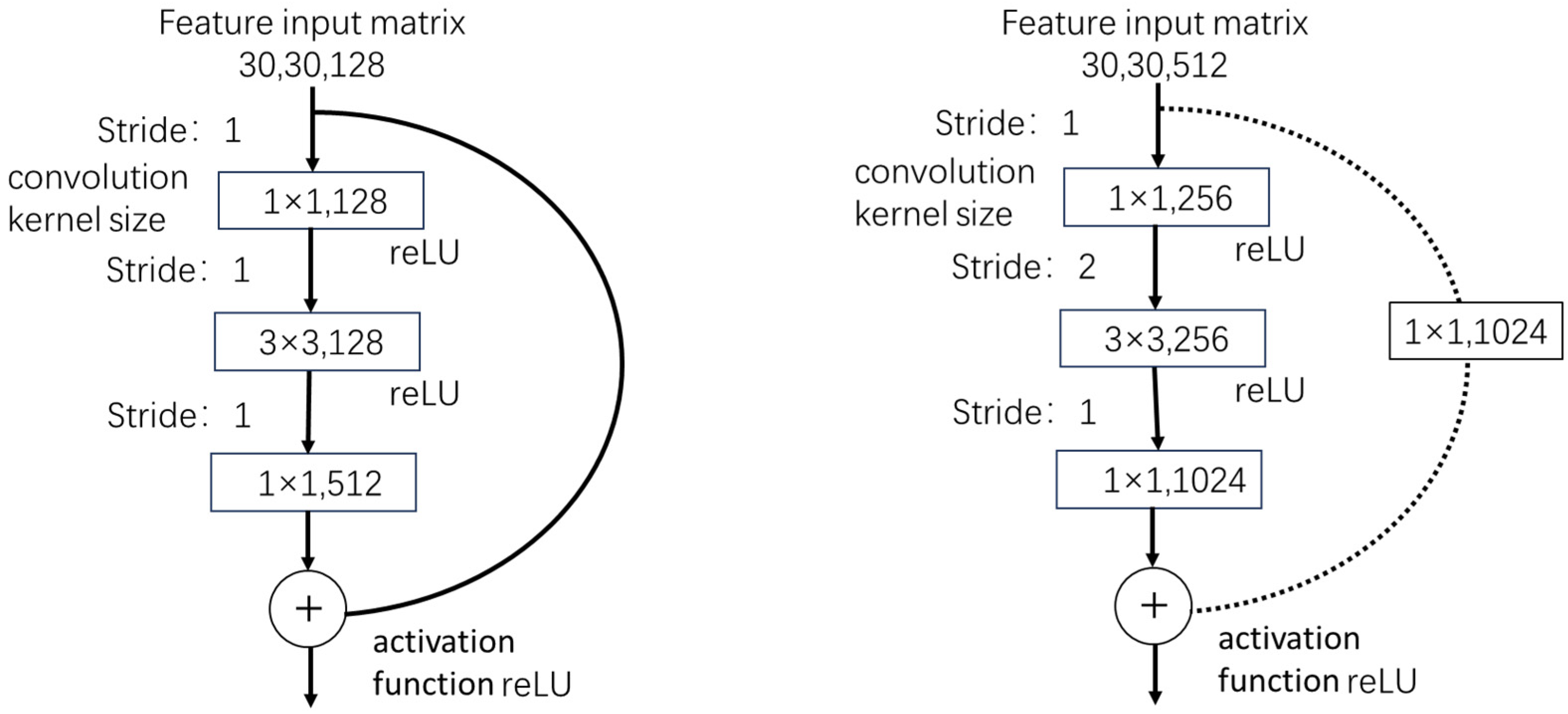
2.3. Dual-Number Residual Structure

The MMDL-Net model is implemented using TensorFlow and comprises four stages, each with a different scale. After comparing ResNet50, ResNet101, and ResNet152, the foundational stage from ResNet50 is retained, which consists of stages with ratios of 3:4:6:3. Unlike traditional computer vision that utilizes RGB images with only three spectral bands, Sentinel-2 images possess 13 spectral bands, and there is also a distinction in the way class labels are defined semantically between computer vision and remote sensing (RS) imagery. Therefore, the channel numbers of these stages are not universally applicable for bridging this semantic gap, which could lead to weaker recognition capabilities for land cover categories. To address this, the channel counts of the stages are doubled, adhering to multiples of two to fully leverage hardware architecture characteristics for enhanced data processing efficiency and performance. This adjustment allows the MMDL-Net model to provide a greater feature representation space to better learn and capture the details and semantic information of the input images, thereby better adapting to complex land use classification tasks. This enhancement ensures improved robustness of the model to variations and noise in the input images, and it increases the accuracy of classification. The channel numbers for each stage are doubled to (128, 256, 512, 1024). Although increasing the number of channels adds to the model’s parameter count and computational complexity, the optimization of modern hardware devices and the TensorFlow framework still allow for the network’s efficient training and inference. The overall structure of the MMDL-Net model is illustrated in Figure 4.

Specifically, channel doubling can be achieved by increasing the number of filters in the 1 × 1 convolutional layers. Within each residual block, a 1 × 1 convolutional layer is used to reduce the number of channels, followed by a 3 × 3 convolutional layer for feature extraction, and finally, another 1 × 1 convolutional layer to increase the number of channels. In the traditional ResNet, the number of filters in these three convolutional layers is c1, c2, and c3, respectively. However, in the MMDL-Net model, we can set the number of filters in these three layers to 2c1, 2c2, and 2c3, respectively, thus doubling the number of channels. In TensorFlow, this increase in the number of channels for each residual block can be achieved by modifying the filter parameters of conv1 and conv2 in the ResBlock class. When using the ResNet model, the number of channels for each residual block can be modified as needed. For example, to increase the number of channels in the first residual block from 64 to 128, one could set filters1 and filters2 to 128, respectively, when defining the MMDL-Net model. In TensorFlow, this will double the number of channels for each residual block, thereby improving the performance of ResNet for remote sensing image classification tasks.

The MMDL-Net model contains multiple residual blocks, with the first residual block having 64 channels. In the channel-doubling enhancement, this block’s channel count is increased from 64 to 128. Similarly, for the other residual blocks, their channel numbers are also doubled. For instance, the channel number of the second residual block is increased from 128 to 256, and the third residual block from 256 to 512, and so on. The two types of residual structures in the MMDL-Net model are shown in Figure 5.

2.4. Multi-Label Classification Module

The BigEarthNet dataset is processed and trained within TensorFlow, being transformed into tensor-type image data. During the classification of remote sensing imagery using the MMDL-Net model, fully connected layers are primarily employed to transform the output feature maps from the convolutional layers into the final classification outputs. These fully connected layers are typically situated at the terminus of the MMDL-Net architecture, accepting a flattened feature vector as input. The initial stages of the MMDL-Net model are dedicated to feature extraction, followed typically by a global average pooling operation. After this operation, the feature maps assume a shape of 1 × 1 × N, where N represents the number of channels. Flattening these feature maps results in a feature vector of length N. This flattened feature vector is then multiplied by a weight matrix, yielding a vector that represents the scores for the various classes. Subsequently, the sigmoid function is adopted as the activation function for the fully connected layer in lieu of the softmax function. This is due to the fact that, in multilabel classification problems, each sample may simultaneously belong to multiple categories rather than a single category. This diverges from the premise of the softmax function, which assumes that each sample can be allocated to only one category, making it suitable for multiclass single-label classification tasks. The softmax function is designed to model a categorical probability distribution over class labels, ensuring that the sum of probabilities of all possible labels for a given sample equals one. This is achieved through the exponentiation and normalization of the output scores from the last layer of the network. However, in the context of remote sensing imagery, where an image may concurrently contain multiple types of land cover, such as water bodies, vegetation, and wetlands, the model should be capable of reflecting the presence of multiple categories. The sigmoid function enables this capacity by being applied independently to each output node, treating the presence of each label as a separate binary classification problem. The fundamental rationale for employing the sigmoid activation function in a multilabel context is that it treats the output for each label independently, which allows the model to represent the probability of the existence of each class label independently. Additionally, as a nonlinear function, it is particularly useful for handling data that possess a high degree of complexity and variability, such as remote sensing imagery. The multiclass infrastructure of the MMDL-Net model is illustrated in Figure 6.

2.5. Construction of the MMDL-Net Loss Function

In TensorFlow, we use the binary cross-entropy loss function, which is easy to compute gradients for and is suitable for multi-label, multi-class tasks without the need for any encoding conversion of labels. In the MMDL-Net model, the output of the fully connected layer is activated through the sigmoid function to obtain the predicted probabilities for each category. Afterward, the binary cross-entropy loss function is used to calculate the discrepancy between the predicted probabilities and the true labels. In multi-label, multi-class tasks, the cross-entropy loss function can effectively be used to compute the loss value of the network and update the network parameters through backpropagation. The formula for the cross-entropy loss function in multi-label, multi-class tasks is as follows:

$$L=-{\displaystyle \sum \left[y\log x+(1-y)\log (1-x)\right]}$$

(3)

Here, $y$ represents the true labels and $x$ represents the predicted values by the network. Both $y$ and $x$ are processed through appropriate encoding to fit the requirements of multi-label multi-class tasks. The formula calculates the prediction $x$ based on the network’s output and the true labels. The predicted results $x$ and the true labels $y$ are input into the cross-entropy loss function formula to calculate the loss value L. Based on the loss value L, the gradient is computed using the backpropagation algorithm, and the network parameters are updated.

During the calculation process, the predicted values need to be processed by an activation function, typically in combination with the sigmoid function, to ensure that their values are between 0 and 1 and that the sum of the predicted probabilities for each class is 1. The Adam algorithm is used for optimization, which updates the network parameters based on the first-order moment estimate and the second-order moment estimate of the parameter gradients. It combines the properties of momentum and adaptive learning rate, enabling efficient optimization of network parameters and improving network performance.

3. Results

3.1. Dataset Introduction and Experimental Configuration

BigEarthNet is a substantial dataset comprised of Earth Observation images, collaboratively developed by the Technical University of Berlin and the German Aerospace Center (DLR). The dataset is designed to advance research in machine learning and deep learning within the remote sensing domain. BigEarthNet encompasses over 590,000 multispectral images captured by the multispectral instrument aboard the Sentinel-2 satellite between the years 2017 and 2018. The dataset’s coverage includes land areas from 10 European countries spanning Western and Northern Europe. Each image in the dataset consists of 13 spectral bands ranging from the visible to the near-infrared spectrum. BigEarthNet is publicly accessible, allowing researchers to download the dataset from its official website (http://bigearth.net/, accessed on 10 August 2023). Detailed information regarding the experimental setup is presented in

Table 2. Detailed information on experimental configurations.

Configuration Item	Details
Deep Learning Library	TensorFlow
software	PyCharm PROFESSIONAL 2019.3
Server	AMAX, Fremont, CA, USA
Graphics Card	NVIDIA GeForce 2080 Ti, Santa Clara, CA, USA
Optimizer	0.001
Training Cycles	500 epochs

.

3.2. Evaluation Metrics

The model is evaluated and monitored using accuracy, precision, recall, and F1 score metrics. By observing changes in accuracy through these metrics, we can discern whether the model is overfitting. Precision allows us to determine how many of the samples predicted as positive by the model are actually positive. Recall shows us how many of the actual positive samples are correctly predicted by the model. The F1 score provides a comprehensive evaluation of the balance between the model’s precision and recall. These metrics help us identify the strengths and shortcomings of the MMDL-Net model and guide us to make necessary adjustments and improvements, thereby enhancing the effectiveness and accuracy of the multi-label classification tasks.

According to the concept of the confusion matrix, a “matching matrix” is often used. Each column in the matrix represents the predicted values, while each row represents the actual categories. It indicates whether there is confusion among multiple categories, that is, whether one class is predicted as another class. By understanding the parameters in

Table 3. Values of different dimensions for calculating evaluation metrics.

	Positive	Negative
True	True Positive (TP)	True Negative (TN)
False	False Positive (FP)	False Negative (FN)

, we can comprehend and calculate the evaluation metrics such as accuracy, precision, recall, and the F1 score.

$$\mathrm{Accuracy}=\frac{\mathrm{T}\mathrm{P}+\mathrm{T}\mathrm{N}}{\mathrm{T}\mathrm{P}+\mathrm{T}\mathrm{N}+\mathrm{F}\mathrm{P}+\mathrm{F}\mathrm{N}}$$

(4)

$$\mathrm{Precision}=\frac{\mathrm{T}\mathrm{P}}{\mathrm{T}\mathrm{P}+\mathrm{F}\mathrm{P}}$$

(5)

$$\mathrm{Recall}=\frac{\mathrm{T}\mathrm{P}}{\mathrm{T}\mathrm{P}+\mathrm{F}\mathrm{N}}$$

(6)

$$\mathrm{F}1=\frac{2\times \mathrm{Precision}\times \mathrm{Recall}}{\mathrm{Precision}+\mathrm{Recall}}$$

(7)

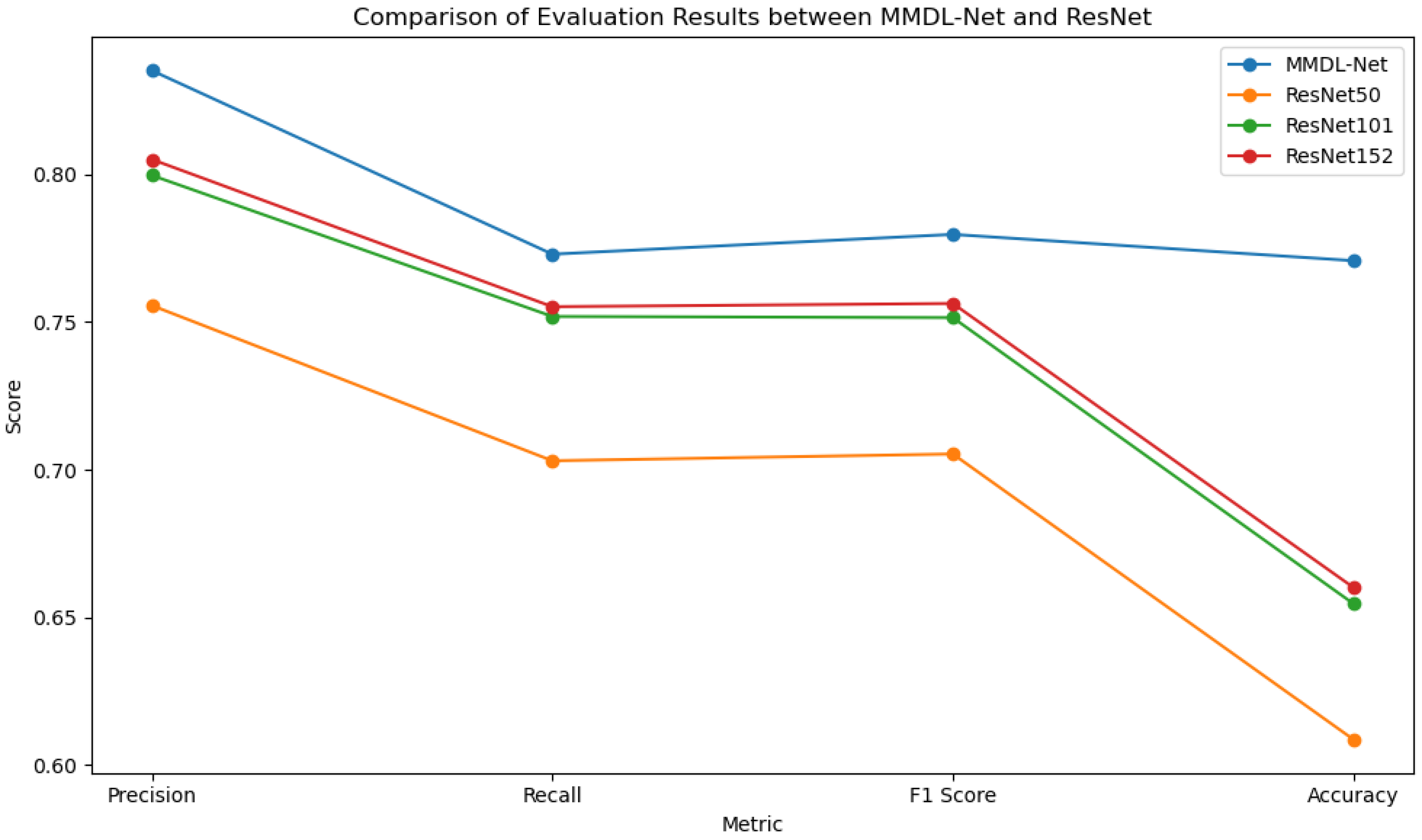
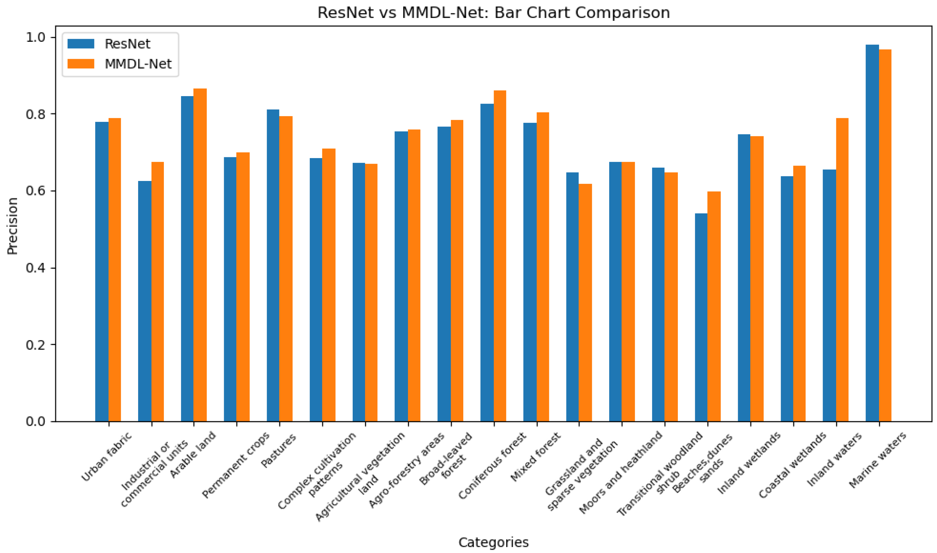
3.3. Result Analysis

In the original BigEarthNet paper [32], the highest precision score achieved by the authors in training was 80.05% for the ResNet50 model. However, with the MMDL-Net model, we achieved a precision score of 83.52%. In a recent study by Papoutsis Ioannis et al. [33], benchmark testing was conducted on the BigEarthNet dataset using 62 DL models for multi-label, multi-class LULC single-image classification tasks. These models included ResNet50, ResNet101, ResNet152, WRN-B4-ECA, among others. The WRN-B4-ECA network achieved the best overall accuracy score of 82.4% for them.

To better evaluate the performance of the models and the improvement achieved, comparative experiments were conducted on ResNet50, ResNet101, ResNet152, and MMDL-Net. The performance metrics of MMDL-Net and ResNet are shown in

Table 4. Performance metrics of MMDL-Net and ResNet.

Model	Precision (%)	Accuracy (%)	Recall (%)	F1 (%)
MMDL-Net	83.52	77.08	77.30	77.97
ResNet50	75.56	60.86	70.30	70.53
ResNet101	79.97	65.46	75.19	75.15
ResNet152	80.51	66.01	75.52	75.63

.

It can be observed that as the network depth increases, the performance gradually improves with ResNet models. However, there is still a significant gap compared to MMDL-Net. This indicates that although deeper network structures can generally capture more complex features and potentially provide better performance to some extent, the performance gain of ResNet tends to plateau as the network depth continues to increase. This suggests that simply increasing the depth of the network is insufficient to adapt to the classification of multi-band, multi-label remote sensing images. This phenomenon may be caused by various factors such as overfitting, vanishing gradients, or saturation of learnable features in the given dataset. However, our MMDL-Net model has been improved in various aspects to better adapt to the classification task of remote sensing images, resulting in better performance than the ResNet model. MMDL-Net and ResNet evaluation results are compared in Figure 7.

Continue to observe the precision of the 19 categories in the application classification of remote sensing images, and it is found that the performance of the MMDL-Net model has improved significantly in most categories. This indicates that our MMDL-Net model has achieved commendable results in these 19 classifications. The precision metrics of the MMDL-Net and three types of ResNet for the 19 categories are shown in

Table 5. Precision metrics for 19 categories of MMDL-Net and three variants of ResNet.

Category	MMDL-Net	ResNet50	ResNet101	ResNet152
Urban buildings	78.43	79.31	76.12	78.21
Commercial and industrial units	65.89	63.36	60.51	63.17
Arable land	85.65	80.81	87.80	85.07
Permanent crops	72.61	68.53	69.62	68.13
Pastures	78.56	83.67	79.56	80.29
Complex farming systems	73.71	68.96	66.58	69.60
Agricultural and vegetation land	71.13	66.20	67.30	67.99
Agroforestry areas	76.82	79.27	71.12	75.95
Broadleaf forests	78.51	74.51	78.25	76.85
Coniferous forests	86.42	76.21	84.72	86.54
Mixed forests	81.38	71.44	81.76	79.56
Grasslands and sparse vegetation	63.54	65.47	66.87	61.98
Swamps and wastelands	65.92	71.35	65.66	64.92
Transitional woodland and shrub	65.03	68.33	64.59	64.98
Beaches, dunes, sandy areas	57.20	57.07	55.28	49.96
Inland wetlands	73.00	71.16	74.94	77.54
Coastal wetlands	67.48	55.75	72.48	62.56
Inland water bodies	87.85	60.32	73.14	72.84
Marine water bodies	96.41	96.98	98.32	98.39

.

Overall, it is evident that the MMDL-Net model outperforms the standard ResNet in most categories. The highest recognition precision occurs in the “Marine water bodies” category, which may be due to their relatively homogenous features that are easier to identify. The lowest recognition precision is observed in the “Beaches, dunes, sand areas” category, possibly because the features of these landforms are more complex and difficult to discern. For landforms such as “Pastures” and “Agroforestry areas”, the performance of the MMDL-Net model is significantly better than that of the standard ResNet, likely due to the superiority of the MMDL-Net model in handling such complex features. The MMDL-Net model performs better when dealing with complex landform features. The average Precision scores for the classification results of MMDL-Net and ResNet are illustrated in Figure 8.

The results above confirm the effectiveness of the MMDL-Net model in the task of remote sensing image classification. Whether compared with the experiments conducted by Sumbul et al. [32], who proposed the BigEarthNet dataset, or the recent benchmark tests conducted by Papoutsis Ioannis et al. [33] on 62 DL models, the MMDL-Net model has demonstrated good performance. However, we also note that the recognition performance of the MMDL-Net model is not very good for certain categories. This may be due to the model’s inability to adapt to individual classifications, resulting in the loss or inadequate extraction of features for such categories. Nevertheless, the introduction of the MMDL-Net model still provides an effective approach for handling remote sensing image data and offers valuable insights for the optimization and improvement of deep learning models for remote sensing images.

4. Discussion

The aim of this study is to fully leverage the information from high-resolution remote sensing images. By processing and analyzing the multi-spectral and multi-band multi-label remote sensing image data, a wealth of geographic information can be obtained, which has extensive applications in various fields. For example, Chen et al. [34] extracted information from mountainous road networks, which is of great significance for road planning, traffic management, and environmental protection in mountainous areas. W. Liu et al. [35] conducted research on identifying agricultural land parcels, providing accurate land use information for agricultural management and decision-making. Wang et al. [36] developed a method for water extraction, which is crucial for water resource management, environmental monitoring, and disaster response. Faisal et al. [37] investigated land cover change, providing important references for urban planning and land management. Shimabukuro et al. [38] studied land use classification, contributing to land management and environmental monitoring in the region. These studies demonstrate the potential of our research in obtaining surface information and assisting scientific research and decision-making processes.

The research findings demonstrate that the MMDL-Net model outperforms the ResNet model in handling categories with complex landform features, such as pastures and agroforestry mixed areas. The MMDL-Net model performs exceptionally well in classifying marine waters, achieving an accuracy of over 95%. Although the accuracy of the MMDL-Net model is slightly lower in categories like beaches, sand dunes, and sandy land, it still shows improvement compared to the ResNet model.

This study involves the identification and classification of various land features, such as forests, farmland, urban areas, water bodies, and natural vegetation. It provides valuable information for decision-making processes related to sustainable development, land management, and conservation efforts. It plays a crucial role in managing land resources, urban planning, environmental monitoring, and natural resource management.

5. Conclusions

To address the issue of accurate classification of multi-band, multi-label, high-resolution remote sensing images, this paper proposes a novel MMDL-Net model. The model introduces a multi-band stacking module and a multi-label classification module and combines a residual network with TensorFlow for feature extraction. It effectively concatenates the information from multiple bands and adjusts the input and output, integrating a multi-label classification strategy to generate more accurate classification outputs. Experimental results demonstrate that the proposed MMDL-Net model exhibits superior classification capability in handling multi-band, multi-label remote sensing image classification. It also performs well in complex remote sensing spatial geographic information. Additionally, the paper explores the impact of changes in network depth and channel numbers on the model.

References

1. Li, Y.; Xu, W.; Chen, H.; Jiang, J.; Li, X. A Novel Framework Based on Mask R-CNN and Histogram Thresholding for Scalable Segmentation of New and Old Rural Buildings. Remote Sens. 2021, 13, 1070. [Google Scholar] [CrossRef]
2. Zerrouki, N.; Harrou, F.; Sun, Y.; Hocini, L. A Machine Learning-Based Approach for Land Cover Change Detection Using Remote Sensing and Radiometric Measurements. IEEE Sens. J. 2019, 19, 5843–5850. [Google Scholar] [CrossRef]
3. Talukdar, S.; Singha, P.; Mahato, S.; Shahfahad; Pal, S.; Liou, Y.-A.; Rahman, A. Land-Use Land-Cover Classification by Machine Learning Classifiers for Satellite Observations—A Review. Remote Sens. 2020, 12, 1135. [Google Scholar] [CrossRef]
4. Dietler, D.; Farnham, A.; de Hoogh, K.; Winkler, M.S. Quantification of Annual Settlement Growth in Rural Mining Areas Using Machine Learning. Remote Sens. 2020, 12, 235. [Google Scholar] [CrossRef]
5. Huang, C.; Zhang, C.; He, Y.; Liu, Q.; Li, H.; Su, F.; Liu, G.; Bridhikitti, A. Land Cover Mapping in Cloud-Prone Tropical Areas Using Sentinel-2 Data: Integrating Spectral Features with Ndvi Temporal Dynamics. Remote Sens. 2020, 12, 1163. [Google Scholar] [CrossRef]
6. Wen, D.; Ma, S.; Zhang, A.; Ke, X. Spatial Pattern Analysis of the Ecosystem Services in the Guangdong-Hong Kong-Macao Greater Bay Area Using Sentinel-1 and Sentinel-2 Imagery Based on Deep Learning Method. Sustainability 2021, 13, 7044. [Google Scholar] [CrossRef]
7. Pan, M.; Hu, T.; Zhan, J.; Hao, Y.; Li, X.; Zhang, L. Unveiling spatiotemporal dynamics and factors influencing the provision of urban wetland ecosystem services using high-resolution images. Ecol. Indic. 2023, 151, 110305. [Google Scholar] [CrossRef]
8. Yang, R.; Ahmed, Z.U.; Schulthess, U.C.; Kamal, M.; Rai, R. Detecting functional field units from satellite images in smallholder farming systems using a deep learning based computer vision approach: A case study from Bangladesh. Remote Sens. Appl. Soc. Environ. 2020, 20, 100413. [Google Scholar] [CrossRef]
9. Lin, C.; Jin, Z.; Mulla, D.; Ghosh, R.; Guan, K.; Kumar, V.; Cai, Y. Toward Large-Scale Mapping of Tree Crops with High-Resolution Satellite Imagery and Deep Learning Algorithms: A Case Study of Olive Orchards in Morocco. Remote Sens. 2021, 13, 1740. [Google Scholar] [CrossRef]
10. Lin, Y.; Wan, L.; Zhang, H.; Wei, S.; Ma, P.; Li, Y.; Zhao, Z. Leveraging optical and SAR data with a UU-Net for large-scale road extraction. Int. J. Appl. Earth Obs. Geoinf. 2021, 103, 102498. [Google Scholar] [CrossRef]
11. Knopp, L.; Wieland, M.; Rättich, M.; Martinis, S. A Deep Learning Approach for Burned Area Segmentation with Sentinel-2 Data. Remote Sens. 2020, 12, 2422. [Google Scholar] [CrossRef]
12. Zheng, X.; Chen, T. Segmentation of High Spatial Resolution Remote Sensing Image based On U-Net Convolutional Networks. In Proceedings of the IGARSS 2020—2020 IEEE International Geoscience and Remote Sensing Symposium, Waikoloa, HI, USA, 26 September–2 October 2020; pp. 2571–2574. [Google Scholar]
13. Yang, J.; Xu, J.; Lv, Y.; Zhou, C.; Zhu, Y.; Cheng, W. Deep learning-based automated terrain classification using high-resolution DEM data. Int. J. Appl. Earth Obs. Geoinf. 2023, 118, 103249. [Google Scholar] [CrossRef]
14. Onojeghuo, A.O.; Miao, Y.; Blackburn, G.A. Deep ResU-Net Convolutional Neural Networks Segmentation for Smallholder Paddy Rice Mapping Using Sentinel 1 SAR and Sentinel 2 Optical Imagery. Remote Sens. 2023, 15, 1517. [Google Scholar] [CrossRef]
15. Ribeiro, T.F.R.; Silva, F.; Moreira, J.; Costa, R.L.d.C. Burned area semantic segmentation: A novel dataset and evaluation using convolutional networks. ISPRS J. Photogramm. Remote Sens. 2023, 202, 565–580. [Google Scholar] [CrossRef]
16. Xu, C.; Gao, M.; Yan, J.; Jin, Y.; Yang, G.; Wu, W. MP-Net: An efficient and precise multi-layer pyramid crop classification network for remote sensing images. Comput. Electron. Agric. 2023, 212, 108065. [Google Scholar] [CrossRef]
17. Sumbul, G.; Charfuelan, M.; Demir, B.; Markl, V. Bigearthnet: A Large-Scale Benchmark Archive for Remote Sensing Image Understanding. In Proceedings of the IGARSS 2019—2019 IEEE International Geoscience and Remote Sensing Symposium, Yokohama, Japan, 28 July–2 August 2019; pp. 5901–5904. [Google Scholar]
18. Manas, O.; Lacoste, A.; Giro-i-Nieto, X.; Vazquez, D.; Rodriguez, P. Seasonal Contrast: Unsupervised Pre-Training from Uncurated Remote Sensing Data. In Proceedings of the 2021 IEEE/CVF International Conference on Computer Vision (ICCV), Montreal, BC, Canada, 11–17 October 2021; pp. 9394–9403. [Google Scholar]
19. Sumbul, G.; Ravanbakhsh, M.; Demir, B. Informative and Representative Triplet Selection for Multilabel Remote Sensing Image Retrieval. IEEE Trans. Geosci. Remote Sens. 2022, 60, 5405811. [Google Scholar] [CrossRef]
20. Stojnic, V.; Risojevic, V. Self-Supervised Learning of Remote Sensing Scene Representations Using Contrastive Multiview Coding. In Proceedings of the 2021 IEEE/CVF Conference on Computer Vision and Pattern Recognition Workshops (CVPRW), Nashville, TN, USA, 19–25 June 2021; pp. 1182–1191. [Google Scholar]
21. Vincenzi, S.; Porrello, A.; Buzzega, P.; Cipriano, M.; Fronte, P.; Cuccu, R.; Ippoliti, C.; Conte, A.; Calderara, S. The color out of space: Learning self-supervised representations for Earth Observation imagery. In Proceedings of the 2020 25th International Conference on Pattern Recognition (ICPR), Milan, Italy, 10–15 January 2021; pp. 3034–3041. [Google Scholar]
22. Diakogiannis, F.I.; Waldner, F.; Caccetta, P.; Wu, C. ResUNet-a: A deep learning framework for semantic segmentation of remotely sensed data. ISPRS J. Photogramm. Remote Sens. 2020, 162, 94–114. [Google Scholar] [CrossRef]
23. Kim, D.-H.; López, G.; Kiedanski, D.; Maduako, I.; Ríos, B.; Descoins, A.; Zurutuza, N.; Arora, S.; Fabian, C. Bias in Deep Neural Networks in Land Use Characterization for International Development. Remote Sens. 2021, 13, 2908. [Google Scholar] [CrossRef]
24. Sumbul, G.; Demir, B. A Deep Multi-Attention Driven Approach for Multi-Label Remote Sensing Image Classification. IEEE Access 2020, 8, 95934–95946. [Google Scholar] [CrossRef]
25. Koßmann, D.; Wilhelm, T.; Fink, G.A. Towards Tackling Multi-Label Imbalances in Remote Sensing Imagery. In Proceedings of the 2020 25th International Conference on Pattern Recognition (ICPR), Milan, Italy, 10–15 January 2021; pp. 5782–5789. [Google Scholar]
26. Dixit, M.; Chaurasia, K.; Kumar Mishra, V. Dilated-ResUnet: A novel deep learning architecture for building extraction from medium resolution multi-spectral satellite imagery. Expert Syst. Appl. 2021, 184, 115530. [Google Scholar] [CrossRef]
27. Rehman, M.u.; Nizami, I.F.; Majid, M. DeepRPN-BIQA: Deep architectures with region proposal network for natural-scene and screen-content blind image quality assessment. Displays 2022, 71, 102101. [Google Scholar] [CrossRef]
28. Wen, L.; Li, X.; Gao, L. A transfer convolutional neural network for fault diagnosis based on ResNet-50. Neural Comput. Appl. 2019, 32, 6111–6124. [Google Scholar] [CrossRef]
29. Sarwinda, D.; Paradisa, R.H.; Bustamam, A.; Anggia, P. Deep Learning in Image Classification using Residual Network (ResNet) Variants for Detection of Colorectal Cancer. Procedia Comput. Sci. 2021, 179, 423–431. [Google Scholar] [CrossRef]
30. Zhou, T.; Chang, X.; Liu, Y.; Ye, X.; Lu, H.; Hu, F. COVID-ResNet: COVID-19 Recognition Based on Improved Attention ResNet. Electronics 2023, 12, 1413. [Google Scholar] [CrossRef]
31. Roy, S.K.; Manna, S.; Song, T.; Bruzzone, L. Attention-Based Adaptive Spectral–Spatial Kernel ResNet for Hyperspectral Image Classification. IEEE Trans. Geosci. Remote Sens. 2021, 59, 7831–7843. [Google Scholar] [CrossRef]
32. Sumbul, G.; Wall, A.d.; Kreuziger, T.; Marcelino, F.; Costa, H.; Benevides, P.; Caetano, M.; Demir, B.; Markl, V. BigEarthNet-MM: A Large-Scale, Multimodal, Multilabel Benchmark Archive for Remote Sensing Image Classification and Retrieval [Software and Data Sets]. IEEE Geosci. Remote Sens. Mag. 2021, 9, 174–180. [Google Scholar] [CrossRef]
33. Papoutsis, I.; Bountos, N.I.; Zavras, A.; Michail, D.; Tryfonopoulos, C. Benchmarking and scaling of deep learning models for land cover image classification. ISPRS J. Photogramm. Remote Sens. 2023, 195, 250–268. [Google Scholar] [CrossRef]
34. Chen, H.; Peng, S.; Du, C.; Li, J.; Wu, S. SW-GAN: Road Extraction from Remote Sensing Imagery Using Semi-Weakly Supervised Adversarial Learning. Remote Sens. 2022, 14, 4145. [Google Scholar] [CrossRef]
35. Liu, W.; Wang, J.; Luo, J.; Wu, Z.; Chen, J.; Zhou, Y.; Sun, Y.; Shen, Z.; Xu, N.; Yang, Y. Farmland Parcel Mapping in Mountain Areas Using Time-Series SAR Data and VHR Optical Images. Remote Sens. 2020, 12, 3733. [Google Scholar] [CrossRef]
36. Wang, B.; Chen, Z.; Wu, L.; Yang, X.; Zhou, Y. SADA-Net: A Shape Feature Optimization and Multiscale Context Information-Based Water Body Extraction Method for High-Resolution Remote Sensing Images. IEEE J. Sel. Top. Appl. Earth Obs. Remote Sens. 2022, 15, 1744–1759. [Google Scholar] [CrossRef]
37. Faisal Koko, A.; Yue, W.; Abdullahi Abubakar, G.; Hamed, R.; Noman Alabsi, A.A. Analyzing urban growth and land cover change scenario in Lagos, Nigeria using multi-temporal remote sensing data and GIS to mitigate flooding. Geomat. Nat. Hazards Risk 2021, 12, 631–652. [Google Scholar] [CrossRef]
38. Shimabukuro, Y.E.; Arai, E.; da Silva, G.M.; Hoffmann, T.B.; Duarte, V.; Martini, P.R.; Dutra, A.C.; Mataveli, G.; Cassol, H.L.G.; Adami, M. Mapping Land Use and Land Cover Classes in São Paulo State, Southeast of Brazil, Using Landsat-8 OLI Multispectral Data and the Derived Spectral Indices and Fraction Images. Forests 2023, 14, 1669. [Google Scholar] [CrossRef]
Figure 1. Structure of the multispectral stacking module.
Applsci 14 02226 g001
Figure 2. Basic structure of the MMDL-Net interpolation method.
Applsci 14 02226 g002
Figure 3. Structure of the MMDL-Net weighted interpolation pixel system.
Applsci 14 02226 g003
Figure 4. Overall structure of the MMDL-Net model.
Applsci 14 02226 g004
Figure 5. The two types of residual structures in the MMDL-Net model.
Applsci 14 02226 g005
Figure 6. The multi-classification basic structure of the MMDL-Net mod.
Applsci 14 02226 g006
Figure 7. Comparison of evaluation results between MMDL-Net and ResNet with three different depths.
Applsci 14 02226 g007
Figure 8. Classification results of the average precision scores for MMDL-Net and ResNet.
Applsci 14 02226 g008