The Genetic Architecture of the Root System during Seedling Emergence in Populus euphratica under Salt Stress and Control Environments

Abstract

The growth of the Populus euphratica root system is of great significance for its survival under adverse environmental stress. In harsh saline-stress environments, the proportion, morphology, and functionality of the taproots and lateral roots and how they manifest specific adaptive structures, growth strategies, and potential genetic controls are still subjects for further exploration. In this study, we delve into the fundamental patterns and trade-offs of root morphology and functionality by constructing an environment-induced differential interaction equation (EDIE) to model the independent and interactive growth of the root system while considering the influence of environmental conditions. We identify 93 key QTLs in the control group and 44 key QTLs in the salt-stress group, of which 2 QTLs are significant in both environments. By constructing ODE-based QTL networks, we explore in depth how these loci regulate the growth of the root system under different environmental conditions while considering their independent direct effects and epistatic effects among loci. This study elucidates the intrinsic factors that influence the variations in taproots and lateral roots, providing crucial insights into the relationship between root morphology and functionality.

1. Introduction

The environment strongly impacts the formation of complex traits and the shaping of plant morphology, i.e., physical appearance [1]. According to the optimal partitioning theory [2], a plant adjusts its biomass allocation strategy to adapt to environmental changes or withstand severe living conditions to capture limited survival resources [3,4,5,6], and its internal mechanisms tend toward homeostasis to maintain regular operation [7].

Soil salinity is one of the most important abiotic stresses threatening plant survival and limiting crop production [8]. Halophytes with strong salt tolerance comprise a small portion of plant species worldwide. Most plant species exhibit reduced growth and productivity under high-salinity conditions [9,10]. Thus, it is necessary to study genetic factors behind salt-resistance mechanisms and genetic solutions to minimize the negative impact of saline environments [11,12]. As an organ in direct contact with soil, the root first perceives the salt environment. It adjusts its biomass allocation in response to salinity stress [13,14,15], resulting in changes in root morphological structure, such as a reduction in taproot elongation and the redistribution of the root mass between the taproot and lateral roots [16]. The adjustment of root morphology further affects the growth and development of plants, as well as the acquisition and utilization of resources [17].

Many studies have focused on the impact of environmental change on the growth of plant biomass allocation [18,19,20] and have linked it with gene regulation, such as determining that different genotypes of specific genes affect biomass allocation [21], cultivating crop varieties with excellent resistance, and using biomass-allocation patterns with technical means to induce genetic variation [22,23]. Several research studies have shown that specific environments can profoundly affect gene networks and circuits [24]. However, few research studies have focused on the genetic-regulation mechanism behind the covariation of phenotypic traits responding to different environmental conditions. Systems mapping is an effective genetic-mapping technique that combines the allometry game theory and association paradigm to identify genetic loci mediating the carbon allocation of two traits and map them throughout the genome [25,26,27]. Using the systems-mapping model, we can clarify how the tree-configuration strategy adjusts in response to environmental changes.

In this paper, we consider cooperation and competition among traits of woody plants to analyze the allocation strategy for photosynthetic products with the changes in the external environment (abiotic stress) (Figure 1). Kolmogorov’s predator–prey model was initially proposed to describe the competition, evolution, and dispersion among species for survival resources [28,29,30]. Combining the characteristics of woody growth from the biophysics perspective with Kolmogorov’s model, we construct EDIE while considering both endogenous and exogenous factors. QTLs are crucial in regulating the development of woody plants. By embedding the EDIE into the systems mapping, some significant Single-Nucleotide Polymorphisms (SNPs) can be identified. Based on genetic effects, regulatory networks are constructed to characterize and visualize these loci’s direct and indirect roadmaps. Our new analytical framework links genotypes to phenotypes to dissect the ecological interplay between traits, incorporating environmental factors into consideration and further capturing how SNPs mediate the dynamic growth pattern. Figure 1 displays the model framework’s schematic diagram implemented in this paper.

Taking seedlings of the hero tree Populus euphratica as an example, it exhibits good salt and drought tolerance [31,32]. Previous research has indicated that under drought conditions, Populus euphratica seedlings undergo significant root phenotypic changes to promote deep rooting, a crucial adaptation strategy for survival [33]. We apply the model to phenotypic and genotypic data from the control and saline-stress groups, aiming to investigate genetic influences behind the growth dynamics between taproot and lateral roots, as well as comprehend how environmental variations impact root-development strategies. Such an analysis clarifies plants’ strategic adjustments when facing environmental change (saline stress) and the genetic mechanisms underlying them. Our framework also provides a reference for cultivating superior varieties with resistance to abiotic stress.

2. Materials and Methods

2.1. Plant Materials

Our study utilized the mapping population data from Populus euphratica that have been previously published [34]. The population is a full-sib F1 family, resulting from the artificial crossbreeding of two dioecious tree specimens. The maternal parent Populus euphratica, Pe-1, and the paternal parent, 0046, originated from the banks of the Tarim River in Korla, Xinjiang, 31 km from each other. In 2014, the male flower branches of paternal parent 0046 were hydroponically cultivated in an artificial climate chamber at Beijing Forestry University (BFU). When the pollen matured, it was collected in EP tubes and refrigerated at −20 °C. The maternal parent Pe-1, Populus euphratica, was transplanted to the greenhouse of BFU. The pollen of paternal parent 0046 was hand-pollinated with the pollen of female flowers at the time of maturity, and mature seeds were successfully harvested in mid-June. Collected seeds were cultured under aseptic conditions in glass tubes, which measured 40 mm in diameter and 400 mm in height. The tubes were filled with a 1/2 Murashige and Skoog medium supplemented with 0.4 mg/L of IBA, 25 g/L of sucrose, and 8 g/L of agar, adjusted to pH 6.0. After being cultivated in tubes for 4 months, 408 seedlings were successfully obtained and transferred to a greenhouse seedbed at BFU for further growth. Following a series of experiments involving histoculture asexualization, expansion, and preservation, a final count of 156 clonal lines demonstrated the plants’ ability to effectively root in the growth medium and mature into fully developed specimens.

To identify the optimal concentration of salt stress, a preliminary experiment was conducted by randomly selecting 20 clonal lines from a pool of 156 Populus euphratica clones. The experiment established four gradients of NaCl concentrations: 0.1%, 0.3%, 0.5%, and 0.7%, corresponding to 17.1116 mM, 51.3347 mM, 85.5578 mM, and 119.781 mM, respectively. These concentrations were tested on the 20 randomly selected clonal lines (with 5 replicates each) through a tube germination culture, aiming to determine the suitable concentration for the trials by observing the growth and development phenotypes of both the aerial parts and the root system. Apical buds, approximately 10 mm in length and containing 4–6 leaves, were inoculated into tubes for cultivation. After 45 days of culture, root formation and survival rates were assessed. The root formation rates under the four NaCl concentration gradients—0.1%, 0.3%, 0.5%, and 0.7%—were found to be 100%, 72%, 5%, and 2%, respectively. Comparing these rates with those of 20 clones under control conditions revealed that a 0.1% NaCl concentration exerted stress on the root growth of Populus euphratica, shortening the taproot length significantly. Consequently, 0.1% NaCl (17.1116 mM) was determined as the necessary concentration for inducing salt stress, ensuring that Populus euphratica saplings could root and grow under such conditions. Moreover, it was observed that most of the tissue-cultured apical buds began to root by the 13th day post-inoculation, which also established the starting point for collecting root trait data.

In vitro inoculation experiments were conducted on 156 clonal lines. Uniformly grown single plants from each clonal line were selected, and apical buds showing consistent growth (approximately 10 mm in length, four to six leaflets) were inoculated into cylindrical flat-bottomed glass tubes measuring 300 mm in length and 45 mm in diameter. Each tube was loaded with 260 milliliters of a growth substrate, and salt-treated tubes contained an additional 0.1% NaCl. Tubes were grouped in sets of 24, and the racks were designed in a 3 by 8 grid pattern. All tube-grown saplings were cultivated in the tissue culture room under uniform conditions with a temperature of 26 °C, light intensity of 1500 lx, and a photoperiod of 16 h of light followed by 8 h of darkness. Data collection commenced on the 13th day post-inoculation. It continued until the 78th day, with measurements of taproot length (TRL, in cm) and lateral root length (LRL, in cm) taken every 5 days for each progeny. All 156 clonal lines demonstrated normal root development and data collection under control conditions, while under salt stress, 117 clonal lines managed to root successfully and yield root growth data.

Leaf samples from the F1 generation were rapidly frozen in liquid nitrogen before being preserved at −80 °C in an ultra-low temperature freezer for further examination. Ge-nomic DNA was extracted using a kit provided by Beijing Tiangen Biotechnology Co., Ltd., Beijing, China, and its purity and concentration were evaluated through agarose gel electrophoresis and quantified with a Nanodrop 2000 spectrophotometer from Thermo Fisher Scientific, Wilmington, DE, USA. Only DNA samples that met the required standards for quality and concentration were forwarded to Megio Biotechnology Co., Ltd., located in Shanghai, for high-throughput sequencing, which was performed on the Illumina HiSeq2500 platform utilizing the restriction enzyme cleavage site-associated DNA (RAD) sequencing approach. Sequencing data were compared with the reference genome [35] using Burrows–Wheeler Aligner (BWA) software v0.7.8. The alignment results were sorted using SAMtools v0.1.18, and of the results produced, 8305 SNPs passed the quality control for association mapping. These SNPs were used to construct a full-sibling population-based genetic linkage map for Populus euphratica, which included 19 linkage groups with a total length of 4574.89 cM and an average distance between markers of 0.55 cM. Based on the principles of Mendelian segregation, the markers were divided into two groups: testcross markers, comprising the types lm × ll and nn × np, and intercross hybrid markers, denoted by hk × hk, with 6886 for the former and 1419 for the latter.

We performed functional annotation and prediction for all significant QTLs using the BLAST tool on the “nucleotide collection (nr/nt)” database at the National Center for Bio-technology Information (NCBI) website (http://blast.ncbi.nlm.nih.gov/) (accessed on 5 January 2024). The comparisons were conducted under the default settings to balance efficiency and accuracy. To ensure the statistical significance of the alignment results, we only retained matches with an E-value less than 0.001.

2.2. Environment-Induced Differential Interaction Equation (EDIE)

The biomass-allocation patterns result in diverse allometric growth relationships, which reflect trees’ trade-offs depending on endogenous biological mechanisms and exogenous factors. The researchers extended the application scenarios of Kolmogorov’s predator–prey model to multiple fields, which can present the relationships between the resource and consumer, vegetation and grazers, and pathogens and hosts, as well as cancerous cells (viruses) and the immune system, among others [28]. EDIE combines Kolmogorov’s model with the characteristics of woody plant growth to quantify the allometry, and it is formulated through two differential equations with a total of 10 parameters to be estimated. The model is expressed as

$$\left\{\begin{array}{c}\frac{d{N}_1}{dt}={\mathsf{\Psi }}_1\left(N_1\right)+{\mathsf{{\rm I}}}_1\left(N_1,N_2\right)+{\epsilon }_1\\ \frac{d{N}_2}{dt}={\mathsf{\Psi }}_2\left(N_2\right)+{\mathsf{{\rm I}}}_2\left(N_1,N_2\right)+{\epsilon }_2\end{array}\right.$$

(1)

where $N_1$ and $N_2$ represent phenotypic values of two characters; ${\mathsf{\Psi }}_1\left(N_1\right)$ and ${\mathsf{\Psi }}_2\left(N_2\right)$ represent the independent growth; ${\mathsf{{\rm I}}}_1\left(N_1,N_2\right)$ and ${\mathsf{{\rm I}}}_2\left(N_1,N_2\right)$ represent the interactive growth; and ${\epsilon }_1$ and ${\epsilon }_2$ represent the environment impact. ${\mathsf{\Psi }}_1\left(N_1\right)$ and ${\mathsf{\Psi }}_2\left(N_2\right)$ are related to the growth characteristics of target traits:

$$\left\{\begin{array}{c}{\mathsf{\Psi }}_1\left(N_1\right)=r_1\cdot N_1\cdot (1-\frac{N_1}{K_1})\\ {\mathsf{\Psi }}_2\left(N_2\right)=r_2\cdot N_2\cdot (1-\frac{N_2}{K_2})\end{array}\right.$$

(2)

where $K_1$ and $K_2$ denote the growth limits for independent growth, and $r_1$ and $r_2$ denote the growth rates for independent growth.

$$\left\{\begin{array}{c}{\mathsf{{\rm I}}}_1\left(N_1,N_2\right)=\alpha \cdot (N_1\cdot N_2)\\ {\mathsf{{\rm I}}}_2\left(N_1,N_2\right)=\beta \cdot (N_1\cdot N_2)\end{array}\right.$$

(3)

symbolizes the interactive growth of lateral root length and taproot length, where $\alpha$ and $\beta$ are the interaction coefficients. These coefficients are designed to quantify how one feature affects the growth rate of the other, reflecting the mutual promotion or inhibition relationship between the features. The values of $\alpha$ and $\beta$ not only indicate the direction of the interaction (positive values indicate a promotion effect, while negative values indicate an inhibition effect), but the magnitude of their absolute values also reflects the strength of the interaction.

$$\left\{\begin{array}{c}{\epsilon }_1={\epsilon }_1\left(t\right)=c_1{e}^{d_{1}t}\\ {{\epsilon }_2=\epsilon }_2\left(t\right)=c_2{e}^{d_{2}t}\end{array}\right.$$

(4)

represents the influence of the environment on plant growth, quantifying how external conditions impact the growth rates of two phenotypic traits, $N_1$ and $N_2$. $c_1$ and $c_2$ denote the magnitude of environmental impact, while $d_1$ and $d_2$ determine the rate at which this impact changes over time. Plants can sense stressful conditions in ecosystems through multiple systems. In our model, ${\epsilon }_1$ and ${\epsilon }_2$ are utilized as composite indices to quantitatively measure the environment’s direct impact on the plant growth rate. These parameters not only illustrate how variations in environmental conditions influence the long-term accumulation of plant biomass but also enable us to model the dynamic effects of environmental factors on plant growth within our mathematical framework.

2.3. Modeling Framework of Systems Mapping

In this study, we incorporate EDIE within systems mapping to identify QTLs influencing the relationship among traits in light of environmental factors [26,36]. The model’s framework relies on a sequence of hypothesis tests across the entire genome. Specifically, in the hypothesis test to determine whether an SNP regulates the interaction growth, the null hypothesis means that the phenotypes of all genotypes are statistically consistent, and the alternative hypothesis indicates that phenotypes of mapping populations with different genotypes are statistically significant.

Let us consider a mapping population of full siblings consisting of n individuals, each genotyped across p SNP markers. We assume that an SNP has $J$ genotypes. ${\overrightarrow{y}}_i=\left({\overrightarrow{y}}_{1i};{\overrightarrow{y}}_{2i}\right)=\left(y_{1i}\left(1\right),y_{1i}\left(2\right),\dots ,y_{1i}\left(T\right);y_{2i}\left(1\right),y_{2i}\left(2\right),\dots ,y_{2i}\left(T\right)\right)$ represents phenotypic values for 2 traits of sample $i$ over a period of time $(t=1,\dots ,\mathrm{T})$. ${\overrightarrow{y}}_i$ follows a bivariate normal distribution characterized by the mean vector $\overrightarrow{\mu }$ and the covariance matrix $\mathsf{\Sigma }$. $\overrightarrow{\mu }$ is fitted by EDIE, corresponding to parameter set ${\mathsf{\Omega }}_{\mu }=\left(K_1,r_1,\alpha ,c_1,d_1,K_2,r_2,\beta ,c_2,d_2\right)$. The matrix Σ is determinable from a parameter set ${\mathsf{\Omega }}_{\mathsf{\Sigma }}$, employing the first-order structured antedependence (SAD(1)) approach [37,38]. $\mathsf{\Omega }=\left({\mathsf{\Omega }}_{\mu };{\mathsf{\Omega }}_{\mathsf{\Sigma }}\right)$ is used to represent the phenotypic value of the target mapping population. A hypothesis test on the parameter set $\mathsf{\Omega }$ is implemented using maximum-likelihood estimation (MLE). The calculation of the test statistic, the log-likelihood ratio (LR), is denoted as

$$LR=-2\left(\mathit{log}\frac{L_0}{L_1}\right)=-2\left(\mathit{log}\frac{{\prod }_{i=1}^{n}f\left({\overrightarrow{y}}_i;\mathsf{\Omega }\right)}{{\prod }_{j=1}^J{\prod }_{i=1}^{n_j}{f}_j({\overrightarrow{y}}_i;{\mathsf{\Omega }}_j)}\right)$$

(5)

where $f\left({\overrightarrow{y}}_i\right)$ is a bivariate probability density function, and where $L_0$ and $L_1$ symbolize the likelihood functions corresponding to the null hypothesis and the alternative hypothesis, respectively. $n_j$ represents the count of samples possessing the genotype $j$ $(j=1,\dots ,J)$, and it satisfies ${\sum }_{j=1}^J{n}_j=n$. During the resolution phase, the fourth-order Runge–Kutta method [39] is employed for solving EDIE, while the Expectation Maximization (EM) algorithm [40,41] is utilized for parameter estimation. Finally, to reduce false positives, the p-value is compared with the critical threshold after applying FDR correction using the Benjamini–Hochberg (BH) method.

2.4. Inferring QTL Networks

The identified significant loci act together as a unified entity influencing root system development. Within this context, each locus exerts its individual role as a direct effect and is influenced by other loci controlling the involved traits, known as epistatic effects. According to the information-based network construction tool proposed by Wu [42], assuming $K$ identified QTLs regulate root system development, we can formulate a set of ordinary differential equations (ODEs), represented as

$$\frac{d{g}_k}{dt}=F_k\left(g_k\left(t\right);{\Theta }_k\right)+\sum _{k^{\prime }=1,k^{\prime }\ne k}^K{F}_{k|k^{\prime }}\left(g_{k^{\prime }}(t);{\Theta }_{k|k^{\prime }}\right),k=1,\cdots K$$

(6)

where the rate of change in genetic effects $g_k\left(t\right)$ of QTL $k$ is divided into the autonomous direct effect, $F_k$(·), alongside the epistatic-dependent effect, $F_{k|k^{\prime }}$(·). The autonomous component of QTL $k$ manifests if the QTL is presumed to be expressed within an isolated environment, driven by its inherent characteristics. The dependent component of QTL $k$ represents the cumulative effect of all other possible QTL $k^{\prime }$ $(k^{\prime }=1,\dots ,K;k^{\prime }\ne k)$ on it. In this study, we employ non-parametric equations, specifically Legendre orthogonal polynomials (LOPs), to model the independent direct effect, $F_k$(·), and the dependent epistatic effect, $F_{k|k^{\prime }}$(·).

For each response QTL $k$, $(K-1)$ predictive elements exist, all influencing the QTL’s epistatic-dependent impact via yet-to-be-determined nonparametric parameters $\left({\Theta }_{k|1},\cdots ,{\Theta }_{k|k-1},{\Theta }_{k|k+1},\cdots ,{\Theta }_{k|K}\right)$. However, depending on the size of the network, there is a limited count of elements in the network that are linked to a specific element [43]. We implement group LASSO [44] to detect the most significant links of $S_k$ $(S_k\ll K)$ that can be used to construct a sparse ODE:

$$\frac{d{g}_k}{dt}=F_k\left(g_k\left(t\right);{\Theta }_k\right)+\sum _{k^{\prime }=1,k^{\prime }\ne k}^{S_k}{F}_{k|k^{\prime }}\left(g_{k^{\prime }}\left(t\right);{\Theta }_{k|k^{\prime }}\right)$$

(7)

We use the least square method to estimate the modified ODE, where parameter estimation is carried out using the fourth-order Runge–Kutta method. We can estimate the dependency effect between a pair of QTLs. These estimated values may be positive, negative, or zero, thereby establishing the causal relationship between the QTLs in the regulation of root growth.

3. Results

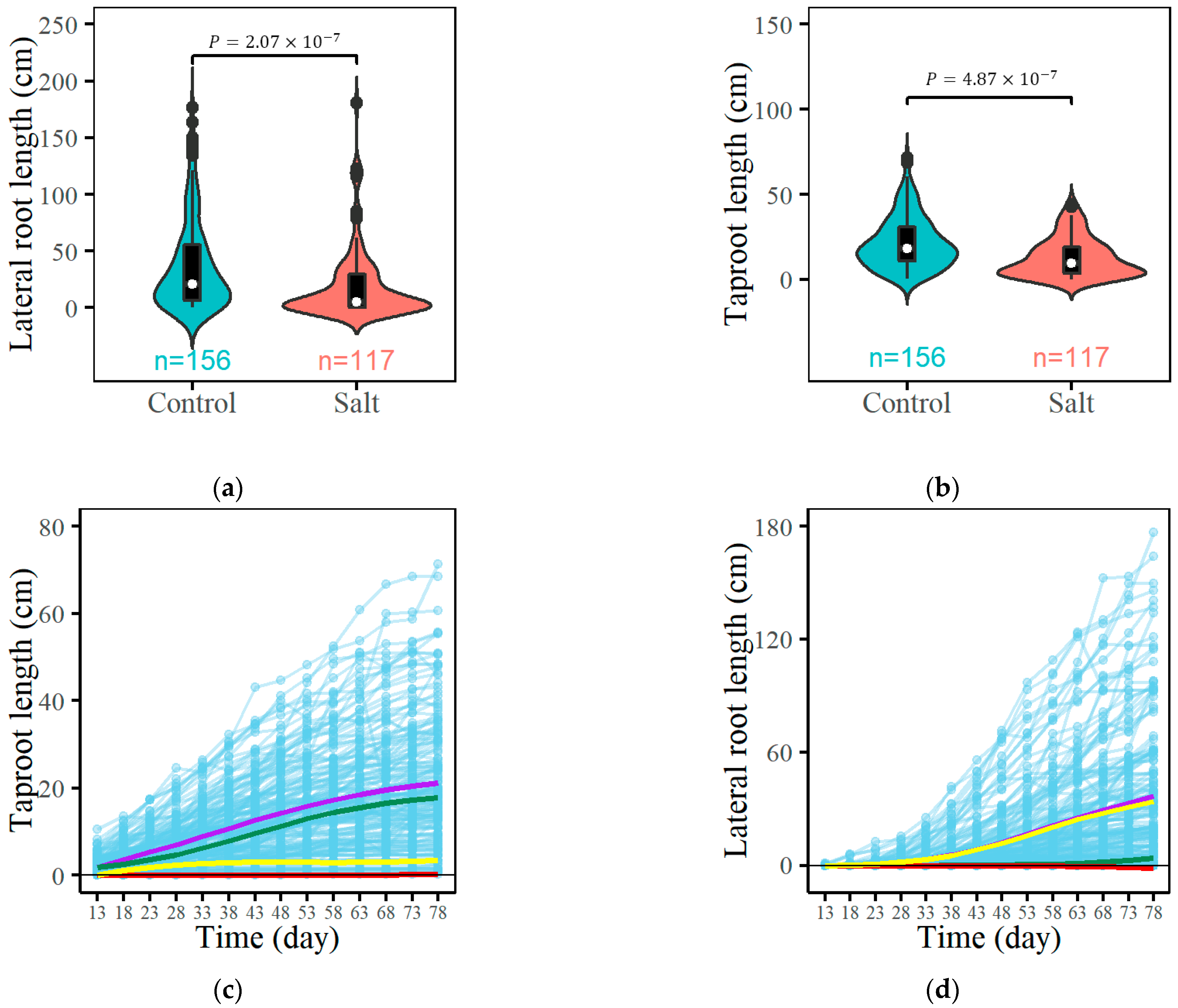
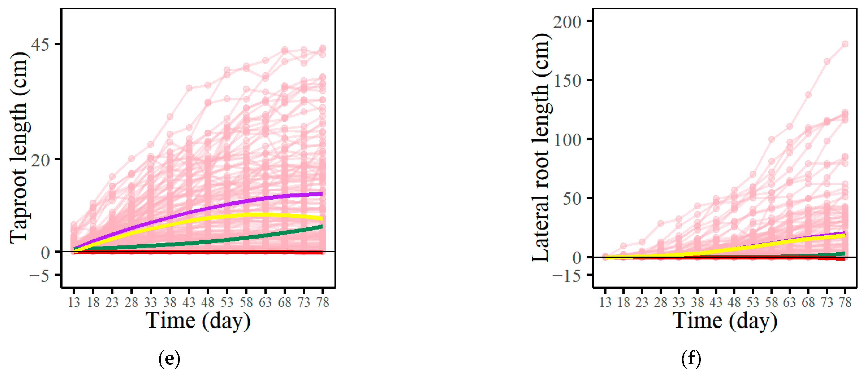
3.1. Growth Trajectory Fitting Based on EDIE

The ecological mapping population includes 156 full-sib individuals of Populus euphratica cultured under salt-free (control) conditions and 117 full-sib individuals cultured under salinity stress (salt). Plants exhibit flexible root phenotypic plasticity by adjusting the biomass allocation of the root system in response to salinity stress, which further affects root system architecture and the underground spatial configuration [45,46]. Here, we choose two representative traits, namely, taproot length and lateral root length, to illustrate the plasticity of root system structure and reveal its genetic potential. As shown in Figure 2a,b, notable differences are visualized between the shape of violins under two cultivation conditions (salt and control). Specifically, the phenotype values of quantitative traits under salt stress are generally lower than those of the control group. The Wilcoxon rank-sum tests confirm these observations, establishing that salt stress significantly impacts root growth (p-value < 0.05).

A two-way ANOVA is used to delve into how the experimental treatments—control and salt-stress conditions—affect root length, alongside the potential interaction between these treatments and root types (taproot vs. lateral roots). The analysis (see Supplementary Table S1) highlights significant main effects for both the treatment condition (F-value = 28.223, p-value < 0.0001) and root type (F-value = 25.156, p-value < 0.0001), underscoring the adverse effects of salinity stress on root lengths and the inherent growth differences between taproots and lateral roots. However, the interaction between treatment and root type is not statistically significant (F-value = 2.734, p-value = 0.0988), indicating a consistent impact of salt stress across both types of roots.

It is noteworthy that there are no 0 values for taproot length observations in the control and salt-stressed groups, whereas 10 out of 156 lateral root length observations are 0 in the control group and 31 out of 117 lateral root length observations are 0 in the salt-stressed group (Supplementary Figure S1). To further understand the incidence of zero values, a Fisher’s exact test was performed (Supplementary Table S1), which showed a significant difference (Odds Ratio = 5.26, p-value = 5.24 $\times$ 10⁻⁶), highlighting the greater likelihood that lateral roots are not malformed under salt stress.

Subsequent Tukey HSD post hoc analyses clarify specific differences between treatments and root types (Supplementary Table S1). The lateral root length is significantly reduced under salt stress compared to the control, with a mean difference of −12.669 cm (<0.0001 ***), highlighting the inhibitory effect of salt on lateral root development. In addition, the intrinsic growth differences between control taproots and lateral roots are also significant, with the most pronounced difference between salt-stressed taproots and control lateral roots, with a mean difference of −23.944 cm (<0.0001 ****).

Figure S2a depicts the allometric growth relationship between the two traits, which helps to understand the relationship between the taproot length and lateral root length and how those relationships change under two cultivation conditions. The purpose of line-fitting indicates that the relationship between two variables has undergone corresponding changes under different processing conditions [47] different from predictions. The fitting results under the two cultivation conditions both indicate a positive correlation between the growth of taproot length and lateral root length. Still, there is a difference in the slope of the two fitted lines, which is due to the saline stress. The distribution of residual values in Figure S2b,c is basically consistent with the normal distribution, meaning that the fitting result is reliable.

Based on the developmental differences in root systems, we use EDIE to fit the growth and game relationships of the taproot-length–lateral-root-length in the control group (Figure 2c,d) and saline-stress group (Figure 2e,f), respectively. The evaluation information presented in

Table 1. The estimated parameters of the taproot and lateral roots fitted based on EDIE and goodness of fit (R²) and residual sum of squares (RSS).

Taproot–Lateral-Root
Control		Saline Stress
Lateral Root	Taproot	Lateral Root	Taproot
31.3696	19.0193	33.4926	22.4966
($K_1$)	($K_2$)	($K_1$)	($K_2$)
0.0815	0.0743	0.0923	0.0368
($r_1$)	($r_2$)	($r_1$)	($r_2$)
−0.0007	0.0004	−0.0028	−0.0007
($\alpha$)	($\beta$)	($\alpha$)	($\beta$)
0.0215	2.3801	0.0221	0.8944
($c_1$)	($c_2$)	($c_1$)	($c_2$)
0.0569	−0.1686	0.0333	−0.0742
($d_1$)	($d_2$)	($d_1$)	($d_2$)
$\mathrm{R}\mathrm{S}\mathrm{S}=$0.8597		$\mathrm{R}\mathrm{S}\mathrm{S}=$0.5530
${\mathrm{R}}^2=$0.9997		${\mathrm{R}}^2=$0.9994

indicates that the fitting based on EDIE exhibits high accuracy. The equation segregates total root growth into independent growth, environmental influences, and interactive growth influenced by another trait. In both environments, the independent growth values for both taproot and lateral root length are smaller than total growth, indicating that root growth benefits from the environment or the coexistence of other traits. It can also be observed that the growth of both the taproot length and lateral length decreases when Populus euphratica is subjected to salt stress. The interaction between the lateral root length and taproot length represents the strategic interplay in root system growth. The figures illustrate that the growth of the taproot inhibits the lateral roots’ growth. In the control group, taproot growth benefits from lateral root growth, whereas under salt stress, lateral root growth inhibits taproot growth, indicating that changes in environmental conditions lead to an adjustment in the strategic interplay of the Populus euphratica root system growth.

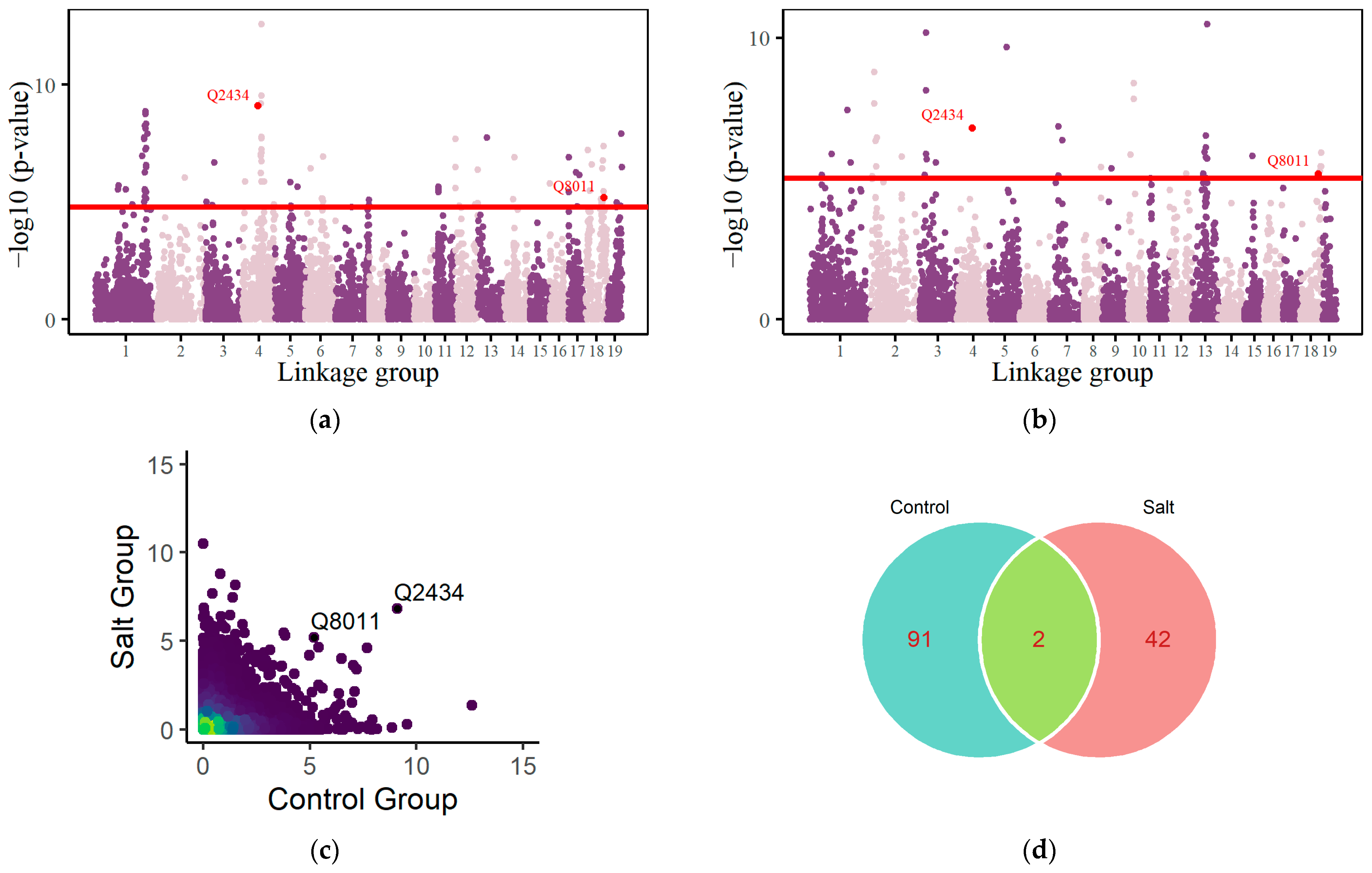
3.2. QTL Mapping of the Root System

According to EDIE, the root system’s growth can be considered a collectively controlled system using parameters $\left(K_1,r_1,\alpha ,c_1,d_1,K_2,r_2,\beta ,c_2,d_2\right)$. Based on Equation (5), we identified 93 significant loci under control group conditions (Figure 3a) and 44 significant loci under salt-stress conditions (Figure 3b) using a threshold of 0.5 $\times$ 10⁻³ after applying the BH method for FDR correction. These loci regulate the growth of both the taproot and lateral roots, as well as the influences of the environment and their interactive relationships. Tables S2 and S3 present the fundamental details of these QTLs, along with annotations on gene functions pertinent to Populus euphratica’s development or homologous genes critical to the development of other tree species. Taking Q2762 (nn_np_3833, Linkage Group 4) as an example, it is linked to a gene encoding a putative F-box/kelch repeat protein. The F-box proteins, constituting a diverse family, are linked to various biological functions in plants [48]. Within this diverse family of proteins, the kelch repeat F-box (KFB) protein subpopulation is an important class. KFB proteins in plants play a role in regulating circadian rhythms, promoting plant development, and regulating secondary metabolic processes [49]. Q1765 (hk_hk_2098, Linkage Group 3) is associated with a gene responsible for encoding E3 ubiquitin-protein ligase HERC2, a key regulator in the cellular DNA-damage-repair process [50].

In the comparison across different environments, the differences in significant loci are evident in their positions within the linkage groups. Under control conditions, significant QTLs predominantly occur within Linkage Groups 1 (28%), 10 (13%), and 14 (17%). In saline-stress conditions, significant QTLs predominantly occur in Linkage Groups 4 (23%), 10 (11%), 12 (16%), and 13 (14%). The differences in significant loci indicate that under different environmental conditions, genes regulating the development strategies of the taproot and lateral roots vary, which also highlights the adaptive strategies of root system growth and development in response to environmental stress. Additionally, two QTLs, Q2434 and Q8011, are found to significantly influence root development across both control scenarios and saline environments (Figure 3c,d). Q2434 (hk_hk_399, Linkage Group 4) encodes uncharacterized LOC110037592. Q8011 (nn_np_6308, Linkage Group 18) encodes LOC105128035, corresponding to a pentatricopeptide repeat-containing (PPR) protein similar to At2g33760. PPR proteins serve numerous essential functions across the life cycle of a plant. They are particularly vital in the processing of RNA within the mitochondria and chloroplasts of plant cells [51].

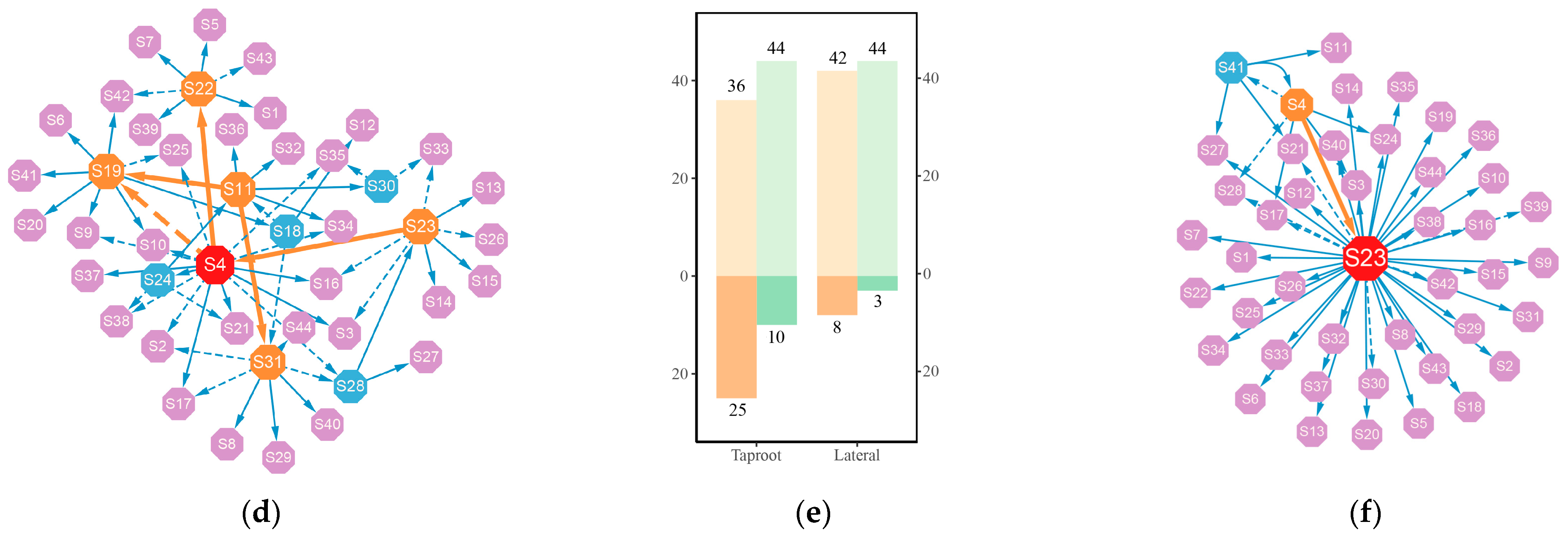
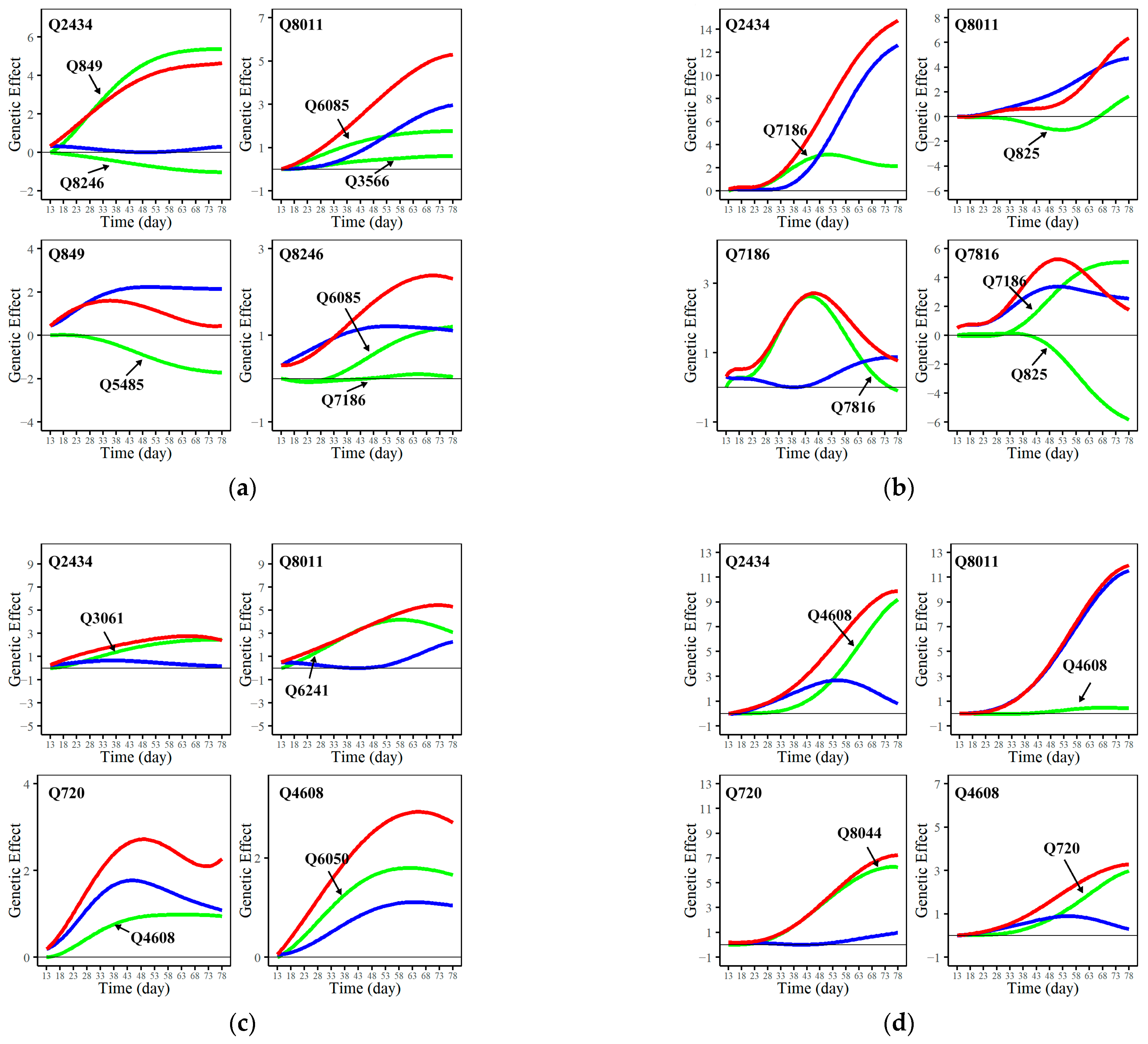
3.3. Genetic Network of Significant QTLs

The systemic growth of the taproot and lateral roots was determined by the effects of 93 QTLs under control group conditions and 44 QTLs under salt-stress conditions and epistatic effects among the QTLs. We utilized a genetic networking strategy grounded in ordinary differential equations (ODEs) to elucidate the interplay among these QTLs within the network and their impact on root development (Figure 4). In a structural analysis of the network, as illustrated in the bar charts, there are 93 and 44 nodes with incoming properties under control and salt-stress conditions, respectively, encompassing all nodes in the network. Therefore, we observe that no node in the network exists independently; each node is subject to the regulatory influence of other nodes. However, only a small subset of nodes has outgoing links, with 22 (23.66%) and 19 (20.43%) nodes in the control group taproot and lateral root networks and 10 (27.73%) and 3 (6.82%) nodes in the salt-stress group taproot and lateral root networks, respectively. These nodes hold stronger leadership positions in the network structure, regulating the expression of the effects of other QTLs. For example, representatives of Q6209, Q7186, and Q7816, namely, S68, S71, and S77, play major regulatory roles in the lateral root network under control conditions. Additionally, there are some minor regulatory nodes, including S5 (Q825), S51 (Q3562), and S87 (Q8016), which are interconnected in the network. According to the functional annotation (Supplementary Tables S2 and S3), the genes where these nodes are located may be functionally associated with plant signal transduction, nucleic acid metabolism, glucose metabolism, and DNA binding.

In our analysis of the genes’ regulatory networks, we quantify complexity based on the proportion of actual connections relative to all possible connections among the QTLs within the network. With regard to the taproot length and lateral root length networks under control conditions, the actual connections represent 1.86% and 1.76% of all potential links, respectively. However, under salt-stress conditions, these proportions increase to 3.22% and 2.64%, respectively. This rise in the percentage of realized connections, despite a significantly lower number of QTLs in the salt-stress networks compared to the control group, signifies a higher network complexity. Here, “complexity” refers to the density of interactions among the QTLs. The increased density of interactions under salt-stress conditions suggests that each QTL may interact with more partners than the control condition, indicating a more intricate web of genetic interactions. QTLs under salt stress achieve stress resistance expression through enhanced mutual regulation. The links between network nodes can be categorized into activating and inhibiting. In terms of quantity, the number of links representing activating interactions is significantly higher than the number of inhibitory links. Moreover, the number of activating interactions becomes even more pronounced under salt stress, which suggests that QTLs exhibit primarily cooperative interactions, coordinating and assisting each other to regulate root growth and confer resistance to adverse environmental influences.

Additionally, we deconstructed QTL structures in the networks, investigating their direct effects on root growth regulation and their epistatic effects influenced by other QTLs. As shown in Figure 5, although both Q2434 and Q8011 regulate root development under control and salt-stressed conditions, their modes of action differ. With regard to taproot growth, Q2434 exhibits shallow independent effects, and its regulatory impact mainly arises from the facilitating effects of other QTLs. In contrast, for lateral roots, Q2434 itself has a certain level of independent effects and is simultaneously influenced by the activating effects of other QTLs. The regulatory effect of Q8011 on the taproot is also enhanced by itself and other loci. However, regarding lateral root growth, its independent direct effects closely align with the overall effects, especially under saline stress, where the epistatic effects induced by Q4608 are close to zero. The regulatory effects of the two QTLs above on the root system are activated by the epistatic effects of other QTLs.

Moreover, within the network structure, certain QTLs, like Q849, play a significant role in the control group. Q849 exhibits a high independent effect in regulating the taproot but is suppressed by Q8246 during the root-growth process. Furthermore, it can be observed in the network structure that the overall regulatory effects on growth, induced by the activation or inhibition from other QTLs, are not consistent. For example, in regulating lateral roots under control conditions, Q7816 is facilitated by Q7186 and inhibited by Q825, resulting in a mutual counteracting effect. If the adverse inhibitory effects are effectively silenced through genetic breeding, Q7816 could enhance root growth and development in Populus euphratica, potentially improving its resilience to adverse conditions. However, it is pertinent to note that genetic improvement may introduce collateral effects on the Gene Regulatory Network (GRN), with many interactions remaining cryptic. Thus, the overall impact on plant physiology remains uncertain, necessitating a careful consideration of genetic modifications within the complex GRN framework.

4. Discussion

A tree’s taproot is typically the root system’s central axis, anchoring the plant underground, preventing lodging, and supporting the entire plant system. In contrast, lateral roots play a crucial role in absorbing water and nutrients, as well as maintaining plant stability [52,53,54]. The growth of taproots and lateral roots is vital in enabling plants to adjust to varied environmental scenarios. Plants in arid or saline–alkali environments may enhance adaptability and stress resistance by adjusting the proportion of taproots and lateral roots [55]. Numerous studies have extensively investigated the QTLs for root growth and their environmental responses [56,57]. However, traditional QTL mapping methods often focus on individual root traits or static growth development at specific time points [58]. Our emphasis lies in the holistic growth system of roots, investigating the dynamic relationships between different traits, such as the length of the taproot and lateral roots. Additionally, we aim to understand the genetic regulation of root growth under environmental stress and its systemic impact. This approach involves a systematic and structured analysis.

In this study, we construct a system of differential equations, namely, the environment-induced differential interaction equation (EDIE), to investigate the growth of the taproot and lateral roots in Populus euphratica. We divided the overall growth into three components, independent growth, interactive growth between traits, and environmental impact, providing a comprehensive analysis of the growth dynamics. The construction of EDIE provides a systematic and highly accurate method for fitting root growth, offering an interpretable tool for exploring the biological significance of growth dynamics. Regardless of salt stress, the growth of both the taproots and lateral roots benefits from environmental influences. This conclusion is reliably evident, as the growth and development of plants rely on obtaining essential growth conditions such as nutrients and water from the environment. While exploring the interactions between traits, we observed that taproot growth inhibits the development of lateral roots. Under control conditions, taproots benefit from lateral root development, an interaction that seems to mirror parasitic relationships in nature. However, under salt-stress conditions, the situation is reversed, and lateral root growth begins to inhibit taproot development, a phenomenon similar to competitive relationships between species in nature. Furthermore, the inhibition effects between the taproots and lateral roots are enhanced. The changes in growth components under environmental stress suggest potential plant growth strategy adjustments.

In QTL mapping, we embedded EDIE into the system mapping framework, successfully locating significant QTLs that regulate root system growth under both control and salt-stress conditions. These QTLs elucidate how Populus euphratica regulates root system growth when confronted with different environmental stresses, contributing to identifying key genes or genetic factors that play pivotal roles in the plant’s adaptability and stress resistance. Furthermore, these QTLs provide potential targets for molecular breeding and genetic improvement. By leveraging these QTLs, plant varieties can be selected and improved to exhibit superior performance under specific environmental conditions.

The QTL mapping results indicate that multiple genes collectively influence the growth of the root system. Constructing an interaction network among these QTLs can aid in identifying and understanding the interactions between different genetic loci, revealing the synergistic effects between them. The flow of information within the network and the identification of hub nodes in the complex network structure unveil the intricate genetic mechanisms underlying quantitative traits. For example, Q7816, which regulates lateral root growth under control conditions, is promoted by Q7186 while being inhibited by Q825.

References

1. Wyatt, J. Grain and Plant Morphology of Cereals and How Characters Can Be Used to Identify Varieties. In Encyclopedia of Food Grains; Elsevier: Amsterdam, The Netherlands, 2016. [Google Scholar] [CrossRef]
2. Bloom, A.J.; Chapin III, F.S.; Mooney, H.A. Resource Limitation in Plants—An Economic Analogy. Annu. Rev. Ecol. Syst. 1985, 16, 363–392. [Google Scholar] [CrossRef]
3. Eziz, A.; Yan, Z.; Tian, D.; Han, W.; Tang, Z.; Fang, J. Drought Effect on Plant Biomass Allocation: A Meta-analysis. Ecol. Evol. 2017, 7, 11002–11010. [Google Scholar] [CrossRef] [PubMed]
4. Gebauer, R.L.; Reynolds, J.F.; Strain, B.R. Allometric Relations and Growth in Pinus Taeda: The Effect of Elevated CO2, and Changing N Availability. New Phytol. 1996, 134, 85–93. [Google Scholar] [CrossRef]
5. Poorter, H.; Niklas, K.J.; Reich, P.B.; Oleksyn, J.; Poot, P.; Mommer, L. Biomass Allocation to Leaves, Stems and Roots: Meta-analyses of Interspecific Variation and Environmental Control. New Phytol. 2012, 193, 30–50. [Google Scholar] [CrossRef]
6. Puglielli, G.; Laanisto, L.; Poorter, H.; Niinemets, Ü. Global Patterns of Biomass Allocation in Woody Species with Different Tolerances of Shade and Drought: Evidence for Multiple Strategies. New Phytol. 2021, 229, 308–322. [Google Scholar] [CrossRef]
7. Freschet, G.T.; Violle, C.; Bourget, M.Y.; Scherer-Lorenzen, M.; Fort, F. Allocation, Morphology, Physiology, Architecture: The Multiple Facets of Plant Above- and Below-ground Responses to Resource Stress. New Phytol. 2018, 219, 1338–1352. [Google Scholar] [CrossRef]
8. Ma, T.; Zeng, W.; Li, Q.; Yang, X.; Wu, J.; Huang, J. Shoot and Root Biomass Allocation of Sunflower Varying with Soil Salinity and Nitrogen Applications. Agron. J. 2017, 109, 2545–2555. [Google Scholar] [CrossRef]
9. Munns, R.; Gilliham, M. Salinity Tolerance of Crops–What Is the Cost? New Phytol. 2015, 208, 668–673. [Google Scholar] [CrossRef]
10. Shahzad, B.; Rehman, A.; Tanveer, M.; Wang, L.; Park, S.K.; Ali, A. Salt Stress in Brassica: Effects, Tolerance Mechanisms, and Management. J. Plant Growth Regul. 2022, 41, 781–795. [Google Scholar] [CrossRef]
11. Ismail, A.M.; Horie, T. Genomics, Physiology, and Molecular Breeding Approaches for Improving Salt Tolerance. Annu. Rev. Plant Biol. 2017, 68, 405–434. [Google Scholar] [CrossRef]
12. Morton, M.J.; Awlia, M.; Al-Tamimi, N.; Saade, S.; Pailles, Y.; Negrão, S.; Tester, M. Salt Stress under the Scalpel–Dissecting the Genetics of Salt Tolerance. Plant J. 2019, 97, 148–163. [Google Scholar] [CrossRef]
13. Galvan-Ampudia, C.S.; Testerink, C. Salt Stress Signals Shape the Plant Root. Curr. Opin. Plant Biol. 2011, 14, 296–302. [Google Scholar] [CrossRef]
14. Luo, D.; Shi, Y.-J.; Song, F.-H.; Li, J.-C. Effects of Salt Stress on Growth, Photosynthetic and Fluorescence Characteristics, and Root Architecture of Corylus Heterophylla× C. avellan Seedlings. Ying Yong Sheng Tai Xue Bao J. Appl. Ecol. 2019, 30, 3376–3384. [Google Scholar] [CrossRef]
15. Lovelli, S.; Scopa, A.; Perniola, M.; Di Tommaso, T.; Sofo, A. Abscisic Acid Root and Leaf Concentration in Relation to Biomass Partitioning in Salinized Tomato Plants. J. Plant Physiol. 2012, 169, 226–233. [Google Scholar] [CrossRef] [PubMed]
16. Julkowska, M.M.; Hoefsloot, H.C.; Mol, S.; Feron, R.; de Boer, G.-J.; Haring, M.A.; Testerink, C. Capturing Arabidopsis Root Architecture Dynamics with ROOT-FIT Reveals Diversity in Responses to Salinity. Plant Physiol. 2014, 166, 1387–1402. [Google Scholar] [CrossRef] [PubMed]
17. Wang, W.; Wang, Y.; Hoch, G.; Wang, Z.; Gu, J. Linkage of Root Morphology to Anatomy with Increasing Nitrogen Availability in Six Temperate Tree Species. Plant Soil 2018, 425, 189–200. [Google Scholar] [CrossRef]
18. Avolio, M.L.; Hoffman, A.M.; Smith, M.D. Linking Gene Regulation, Physiology, and Plant Biomass Allocation in Andropogon Gerardii in Response to Drought. Plant Ecol. 2018, 219, 1–15. [Google Scholar] [CrossRef]
19. Liu, R.; Yang, X.; Gao, R.; Hou, X.; Huo, L.; Huang, Z.; Cornelissen, J.H. Allometry Rather than Abiotic Drivers Explains Biomass Allocation among Leaves, Stems and Roots of Artemisia across a Large Environmental Gradient in China. J. Ecol. 2021, 109, 1026–1040. [Google Scholar] [CrossRef]
20. Zhang, Y.; Zheng, Q.; Gao, X.; Ma, Y.; Liang, K.; Yue, H.; Huang, X.; Wu, K.; Wang, X. Land Degradation Changes the Role of Above-and Belowground Competition in Regulating Plant Biomass Allocation in an Alpine Meadow. Front. Plant Sci. 2022, 13, 822594. [Google Scholar] [CrossRef]
21. Ribeiro, P.R.; Zanotti, R.F.; Deflers, C.; Fernandez, L.G.; de Castro, R.D.; Ligterink, W.; Hilhorst, H.W. Effect of Temperature on Biomass Allocation in Seedlings of Two Contrasting Genotypes of the Oilseed Crop Ricinus Communis. J. Plant Physiol. 2015, 185, 31–39. [Google Scholar] [CrossRef] [PubMed]
22. OlaOlorun, B.M.; Shimelis, H.A.; Mathew, I. Variability and Selection among Mutant Families of Wheat for Biomass Allocation, Yield and Yield-related Traits under Drought-stressed and Non-stressed Conditions. J. Agron. Crop Sci. 2021, 207, 404–421. [Google Scholar] [CrossRef]
23. Shamuyarira, K.W.; Shimelis, H.; Mathew, I.; Zengeni, R.; Chaplot, V. A Meta-analysis of Combining Ability Effects in Wheat for Agronomic Traits and Drought Adaptation: Implications for Optimizing Biomass Allocation. Crop Sci. 2022, 62, 139–156. [Google Scholar] [CrossRef]
24. López-Pérez, M.; Aguirre-Garrido, F.; Herrera-Zúñiga, L.; Fernández, F.J. Gene as a Dynamical Notion: An Extensive and Integrative Vision. Redefining the Gene Concept, from Traditional to Genic-Interaction, as a New Dynamical Version. Biosystems 2023, 234, 105060. [Google Scholar] [CrossRef]
25. Fu, L.; Sun, L.; Hao, H.; Jiang, L.; Zhu, S.; Ye, M.; Tang, S.; Huang, M.; Wu, R. How Trees Allocate Carbon for Optimal Growth: Insight from a Game-Theoretic Model. Brief. Bioinform. 2018, 19, 593–602. [Google Scholar] [CrossRef]
26. Sun, L.; Wu, R. Mapping Complex Traits as a Dynamic System. Phys. Life Rev. 2015, 13, 155–185. [Google Scholar] [CrossRef]
27. Wu, R.; Lin, M. Functional Mapping—How to Map and Study the Genetic Architecture of Dynamic Complex Traits. Nat. Rev. Genet. 2006, 7, 229–237. [Google Scholar] [CrossRef] [PubMed]
28. Brauer, F.; Castillo-Chavez, C.; Castillo-Chavez, C. Mathematical Models in Population Biology and Epidemiology; Springer: Berlin/Heidelberg, Germany, 2012; Volume 2. [Google Scholar] [CrossRef]
29. Freedman, H.I. Deterministic Mathematical Models in Population Ecology; M. Dekker: New York, NY, USA, 1980; Volume 38, pp. 876–877. [Google Scholar] [CrossRef]
30. Hoppensteadt, F. Predator-Prey Model. Scholarpedia 2006, 1, 1563. [Google Scholar] [CrossRef]
31. Si, J.; Zhou, T.; Bo, W.; Xu, F.; Wu, R. Genome-Wide Analysis of Salt-Responsive and Novel microRNAs in Populus euphratica by Deep Sequencing. In BMC Genetics; BioMed Central: London, UK, 2014; Volume 15, pp. 1–11. [Google Scholar] [CrossRef]
32. Yao, J.; Shen, Z.; Zhang, Y.; Wu, X.; Wang, J.; Sa, G.; Zhang, Y.; Zhang, H.; Deng, C.; Liu, J. Populus euphratica WRKY1 Binds the Promoter of H+-ATPase Gene to Enhance Gene Expression and Salt Tolerance. J. Exp. Bot. 2020, 71, 1527–1539. [Google Scholar] [CrossRef]
33. Ye, Z.; Wang, J.; Wang, W.; Zhang, T.; Li, J. Effects of Root Phenotypic Changes on the Deep Rooting of Populus euphratica Seedlings under Drought Stresses. PeerJ 2019, 7, e6513. [Google Scholar] [CrossRef]
34. Zhang, M.M. QTL Mapping and Epistatic Analysis of the Response of Populus euphratica Root Growth Dynamics to Salt Stress. Ph.D. Thesis, Beijing Forestry University, Beijing, China, 2019. [Google Scholar] [CrossRef]
35. Ma, T.; Wang, J.; Zhou, G.; Yue, Z.; Hu, Q.; Chen, Y.; Liu, B.; Qiu, Q.; Wang, Z.; Zhang, J.; et al. Genomic Insights into Salt Adaptation in a Desert Poplar. Nat. Commun. 2013, 4, 2797. [Google Scholar] [CrossRef]
36. Wu, R.; Cao, J.; Huang, Z.; Wang, Z.; Gai, J.; Vallejos, E. Systems Mapping: How to Improve the Genetic Mapping of Complex Traits through Design Principles of Biological Systems. BMC Syst. Biol. 2011, 5, 84. [Google Scholar] [CrossRef]
37. Jaffrézic, F.; Thompson, R.; Hill, W.G. Structured Antedependence Models for Genetic Analysis of Repeated Measures on Multiple Quantitative Traits. Genet. Res. 2003, 82, 55–65. [Google Scholar] [CrossRef]
38. Zhao, W.; Chen, Y.Q.; Casella, G.; Cheverud, J.M.; Wu, R. A Non-Stationary Model for Functional Mapping of Complex Traits. Bioinformatics 2005, 21, 2469–2477. [Google Scholar] [CrossRef]
39. Blum, E.K. A Modification of the Runge-Kutta Fourth-Order Method. Math. Comput. 1962, 16, 176–187. [Google Scholar] [CrossRef]
40. Do, C.B.; Batzoglou, S. What Is the Expectation Maximization Algorithm? Nat. Biotechnol. 2008, 26, 897–899. [Google Scholar] [CrossRef]
41. Moon, T.K. The Expectation-Maximization Algorithm. IEEE Signal Process. Mag. 1996, 13, 47–60. [Google Scholar] [CrossRef]
42. Wu, R.; Jiang, L. Recovering Dynamic Networks in Big Static Datasets. Phys. Rep. 2021, 912, 1–57. [Google Scholar] [CrossRef]
43. Busiello, D.M.; Suweis, S.; Hidalgo, J.; Maritan, A. Explorability and the Origin of Network Sparsity in Living Systems. Sci. Rep. 2017, 7, 12323. [Google Scholar] [CrossRef] [PubMed]
44. Yuan, M.; Lin, Y. Model Selection and Estimation in Regression with Grouped Variables. J. R. Stat. Soc. Ser. B Stat. Methodol. 2006, 68, 49–67. [Google Scholar] [CrossRef]
45. Dinneny, J.R. Developmental Responses to Water and Salinity in Root Systems. Annu. Rev. Cell Dev. Biol. 2019, 35, 239–257. [Google Scholar] [CrossRef] [PubMed]
46. Korver, R.A.; van den Berg, T.; Meyer, A.J.; Galvan-Ampudia, C.S.; Ten Tusscher, K.H.; Testerink, C. Halotropism Requires Phospholipase Dζ1-mediated Modulation of Cellular Polarity of Auxin Transport Carriers. Plant Cell Environ. 2020, 43, 143–158. [Google Scholar] [CrossRef]
47. Warton, D.I.; Duursma, R.A.; Falster, D.S.; Taskinen, S. Smatr 3–an R Package for Estimation and Inference about Allometric Lines. Methods Ecol. Evol. 2012, 3, 257–259. [Google Scholar] [CrossRef]
48. Zhang, X.; Gonzalez-Carranza, Z.H.; Zhang, S.; Miao, Y.; Liu, C.-J.; Roberts, J.A. F-Box Proteins in Plants. Annu Plant Rev 2019, 2, 307–328. [Google Scholar] [CrossRef]
49. ul Hassan, M.N.; Zainal, Z.; Ismail, I. Plant Kelch Containing F-Box Proteins: Structure, Evolution and Functions. RSC Adv. 2015, 5, 42808–42814. [Google Scholar] [CrossRef]
50. Mathieu, N.A.; Levin, R.H.; Spratt, D.E. Exploring the Roles of HERC2 and the NEDD4L HECT E3 Ubiquitin Ligase Subfamily in P53 Signaling and the DNA Damage Response. Front. Oncol. 2021, 11, 659049. [Google Scholar] [CrossRef] [PubMed]
51. Li, X.; Sun, M.; Liu, S.; Teng, Q.; Li, S.; Jiang, Y. Functions of PPR Proteins in Plant Growth and Development. Int. J. Mol. Sci. 2021, 22, 11274. [Google Scholar] [CrossRef] [PubMed]
52. Comas, L.H.; Eissenstat, D.M. Patterns in Root Trait Variation among 25 Co-existing North American Forest Species. New Phytol. 2009, 182, 919–928. [Google Scholar] [CrossRef] [PubMed]
53. Hodge, A. Root Decisions. Plant Cell Environ. 2009, 32, 628–640. [Google Scholar] [CrossRef] [PubMed]
54. Lynch, J. Root Architecture and Plant Productivity. Plant Physiol. 1995, 109, 7. [Google Scholar] [CrossRef] [PubMed]
55. Bengough, A.G.; McKenzie, B.M.; Hallett, P.D.; Valentine, T.A. Root Elongation, Water Stress, and Mechanical Impedance: A Review of Limiting Stresses and Beneficial Root Tip Traits. J. Exp. Bot. 2011, 62, 59–68. [Google Scholar] [CrossRef]
56. Atkinson, J.A.; Wingen, L.U.; Griffiths, M.; Pound, M.P.; Gaju, O.; Foulkes, M.J.; Le Gouis, J.; Griffiths, S.; Bennett, M.J.; King, J. Phenotyping Pipeline Reveals Major Seedling Root Growth QTL in Hexaploid Wheat. J. Exp. Bot. 2015, 66, 2283–2292. [Google Scholar] [CrossRef] [PubMed]
57. Qu, Y.; Mu, P.; Zhang, H.; Chen, C.Y.; Gao, Y.; Tian, Y.; Wen, F.; Li, Z. Mapping QTLs of Root Morphological Traits at Different Growth Stages in Rice. Genetica 2008, 133, 187–200. [Google Scholar] [CrossRef] [PubMed]
58. Pierret, A.; Moran, C.J.; Doussan, C. Conventional Detection Methodology Is Limiting Our Ability to Understand the Roles and Functions of Fine Roots. New Phytol. 2005, 166, 967–980. [Google Scholar] [CrossRef] [PubMed]
Figure 1. Conceptual illustration of the model structure. The model is applied to phenotypic growth data of control and salt-stressed Populus euphratica seedlings to pinpoint crucial loci regulating trait growth through EDIE-based systems mapping and constructing genetic networks so as to explore the potential genetic mechanisms of taproot-length–lateral-root-length growth and understand the effects of environmental changes on root-growth strategies.
Applsci 14 02225 g001
Figure 2. Analysis of the development of seedlings within a full-sibling group of Populus euphratica. Violin plots contrasting taproot (a) and lateral root lengths (b) under control versus saline environments. Growth curves for both taproot and lateral root length depicted across control (c,d) versus saline-exposure scenarios (e,f). Each purple trajectory represents the average growth trend of the corresponding trait, which consists of independent growth (green trajectories), interactive growth with another trait (red trajectories), and environmental effects (yellow trajectories). Here, “average growth” is defined as the arithmetic mean of growth measurements across observations, providing a statistical estimate for the expected growth pattern under each condition.
Applsci 14 02225 g002aApplsci 14 02225 g002b
Figure 3. Manhattan plot of p-values across 19 linkage groups of Populus euphratica under control (a) and salt-stress conditions (b), with the significance threshold (red horizontal line) established using the Benjamini–Hochberg (BH) method for FDR correction. Red dots indicate QTLs that are significant in both control and salt-stress groups. (c) Density plot of QTLs identified in control and salt-stress groups. (d) Venn Diagram for QTLs identified within both control and salt-stress scenarios.
Applsci 14 02225 g003
Figure 4. The taproot length genetic effects network (a) versus the lateral root length genetic effects network (c) in the control group. (b) Bar charts depict activating/inhibitory links and outgoing/incoming nodes for taproot length and lateral root length networks in the control group. The taproot length genetic effects network (d) versus the lateral root length genetic effects network (f) in the salt-stress group. (e) Bar charts depict activating/inhibitory links and outgoing/incoming nodes for taproot length and lateral root length networks in the salt-stressed group. Each node symbolizes a QTL. The lines between nodes illustrate QTL interactions, with dotted lines indicating inhibition and solid lines denoting facilitation. Red, orange, and blue nodes indicate that this QTL has a stimulatory or inhibitory effect on other QTLs. The red nodes are hub QTLs, the orange nodes are secondary hub QTLs, and the blue nodes are tertiary hub QTLs.
Applsci 14 02225 g004aApplsci 14 02225 g004b
Figure 5. Genetic effect curves for specific QTLs in the genetic network for control taproot length (a), control lateral root length (b), salt-stressed taproot length (c), and salt-stressed lateral root length (d). The net genetic effect (red line) is divided into independent effects (blue line) and dependent effects (green line) due to regulation by other QTLs.
Applsci 14 02225 g005