Routing Control Optimization for Autonomous Vehicles in Mixed Traffic Flow Based on Deep Reinforcement Learning

Abstract

With recent technological advancements, the commercialization of autonomous vehicles (AVs) is expected to be realized soon. However, it is anticipated that a mixed traffic of AVs and human-driven vehicles (HVs) will persist for a considerable period until the Market Penetration Rate reaches 100%. During this phase, AVs and HVs will interact and coexist on the roads. Such an environment can cause unpredictable and dynamic traffic conditions due to HVs, which results in traffic problems including traffic congestion. Therefore, the routes of AVs must be controlled in a mixed traffic environment. This study proposes a multi-objective vehicle routing control method using a deep Q-network to control the driving direction at intersections in a mixed traffic environment. The objective is to distribute the traffic flow and control the routes safely and efficiently to their destination. Simulation results showed that the proposed method outperformed existing methods in terms of the driving distance, time, and waiting time of AVs, particularly in more dynamic traffic environments. Consequently, the traffic became smooth as it moved along optimal routes.

1. Introduction

With the rapid development of information communication and artificial intelligence (AI) technologies, autonomous driving technologies have attracted considerable attention as the core of future mobility. Autonomous vehicles (AVs) refer to cars that can drive independently without direct driver manipulation. Autonomous driving technology is classified into six levels (levels 0–5), and levels 3–5 are generally classified as AVs [1]. AVs can actively drive, and they can avoid potential risks by receiving information about the surrounding road conditions and nearby vehicles through Vehicle-to-Vehicle (V2V) and Vehicle-to-Infrastructure (V2I) communication. AVs have demonstrated positive effects in the context of various perspectives such as road safety, traffic capacity, and mobility [2]. Moreover, AVs can potentially solve traffic-related problems, such as traffic congestion.

South Korea is currently in the demonstration stage, with the goal of commercializing Level 4 autonomous driving by 2027. The annual growth rate of the AV-related industry in North America, Western Europe, and the Asia–Pacific region is anticipated to be about 85% from 2020 to 2035 [3]. In addition, the Market Penetration Rate (MPR) of AVs is expected to reach approximately 75% by the year 2035. In the autonomous driving environment, it is anticipated that mixed traffic of AVs and human-driven vehicles (HVs) will persist for a considerable period until the MPR reaches 100% [4]. During this transitional phase, AVs and HVs will interact and coexist on the roads. The coexistence of AVs and HVs in a traffic environment has the potential to induce unstable traffic flow, thus negatively impacting safety by increasing the frequency and severity of traffic accidents [5].

Therefore, to optimize traffic flow in a mixed traffic system, high-level decision making in AVs is essential as it can ensure that both AVs and HVs reach their destinations safely and efficiently. One of the major challenges in the high-level decision making of AVs is the vehicle routing problem (VRP) [6,7], which significantly influences traffic safety and efficiency. Research on VRP, which aims to find efficient routes to destinations, has been extensively conducted; however, these studies have been insufficient in considering mixed traffic systems. In a mixed traffic system, HVs are likely to cause unpredictable and dynamic traffic conditions because they are driven by humans. Consequently, as HVs bring unknown/uncertain behaviors, planning, and control in such mixed traffic systems, achieving safe and efficient maneuvers is challenging [8]. Therefore, efficient methods for controlling the routing of AVs while considering mixed traffic environments of AVs and HVs are needed.

However, there is a limit to AV routing control when using deep learning in a dynamic environment that changes in real time. In other words, a large amount of labeled data is required to achieve good results with deep learning. However, it is difficult to generate such data for the complex decision-making process of autonomous driving when using deep learning. Therefore, it is crucial to demonstrate how to process these decisions without using explicitly labeled data or predefined rules. Deep reinforcement learning (DRL) is a potential machine learning method that can address this problem.

Therefore, we propose a DRL method that utilizes a deep Q-network (DQN) [9] for AV route control. This method features a novel local reward design that incorporates safety and efficiency. Additionally, the AVs learn policies to alleviate traffic congestion by reflecting local information such as real-time traffic. The AVs aim to make necessary route control for efficiency improvement while ensuring safe traffic movement in a mixed traffic system. The contributions of this study can be summarized as follows:

• We formulate a model of vehicle routing control that reflects real-time local information in mixed traffic as a decentralized problem, where agents learn a safe and efficient driving policy to distribute traffic flow and improve efficiency.
• We proposed a novel, efficient, and scalable routing control model by introducing an effective reward function design.
• We conduct comparative experiments on various MPR values and traffic densities, as well as demonstrate the model in terms of driving safety and efficiency compared to other conventional models.

The remainder of this paper is organized as follows. Section 2 introduces the related studies. Section 3 describes the vehicle routing control method using a DQN. Section 4 discusses the experimental results. Finally, Section 5 presents the main conclusions of this study.

2. Related Works

In this section, we introduce conventional studies on vehicle routing control to solve the VRP. Many studies have been conducted to find the optimal route from the origin to the destination for the purpose of achieving a minimum distance, minimum cost, or minimum driving time [10,11,12]. These studies generally used metaheuristic algorithms, including particle swarm optimization (PSO), a genetic algorithm (GA), and ant colony optimization (ACO). In [10], the authors used the PSO algorithm to minimize carbon emissions, waiting times, and the number of vehicles. PSO is an optimization algorithm in which particles (simple entities forming a cluster) share their experiences in finding a solution to a problem. The vehicle load and driving distance were modeled to achieve these objectives. The study in [11] addressed the vehicle routing problem using a GA, which determines optimal solutions by imitating the evolution of organisms as they adapt to their environment. The objective was to minimize the total driving distance of vehicles with capacity and distance constraints. In addition, the study of [12] proposed energy-efficient vehicle-optimized routing, which utilized the ACO (expressed by the energy consumption and speed of an AV) to maximize energy efficiency. However, these vehicle routing methods, such as navigation systems that find the optimal distance from the origin to the destination, may inadvertently cause temporary traffic congestion by suggesting similar routes when neighboring vehicles have the same destination. These methods make decisions based on global information for global optimization, which may hinder their ability to quickly adapt to changes in road conditions or traffic due to insufficient real-time traffic updates.

Therefore, to alleviate traffic congestion, it requires not only global decisions, but also local decisions that enable real-time route updates based on current traffic volume. Existing studies have introduced methods for controlling vehicle routes that make local decisions based on real-time local traffic information, which can be mainly classified into two categories: lane changing and direction changing. Local traffic information reflects not only the current state, but also the localized conditions and factors related to the surroundings. By leveraging this information, agents can better understand their surrounding environment and respond appropriately to the state. This intelligent behavior combines the right choices for the current state in which the surroundings are considered, thus ultimately leading to global optimality.

First of all, a lane changing approach aims to enable vehicles to safely and quickly reach their destinations by controlling the lane changing within the same direction of driving at the edge level of roads. Many DRL-based methods have been proposed for the purpose of learn lane changing behavior based on real-time local information such as the state of nearby vehicles, [13,14,15,16]. The studies have focused on training AVs to intelligently perform lane changing. In [13,14], the authors proposed a lane changing method that determines whether to change lanes for a safe, smooth, and efficient lane changing. In [15], the authors proposed a method to determine whether to keep the current lane, change it to the right lane, or change it to the left lane for high-speed driving. In addition, a method for determining acceleration and deceleration beyond lane changing has also been proposed [16]. However, lane changing is aimed at ensuring efficient and safe driving at the edge level of roads, i.e., controlling lane changes within the same route and direction of driving. In other words, lane changing usually involves controlling lanes without altering the overall route, thus not effectively distributing the overall traffic flow and congestion.

Therefore, from a microscopic perspective, it requires direction changing to distribute the route by controlling the driving direction at the node level of the road, which is an intersection. This reduces traffic congestion and allows the vehicles to reach their destination quickly and efficiently. For instance, in the case of a four-way intersection, it is to determine the driving direction for a left turn, a right turn, or a straight one by considering the real-time local traffic situation of the intersection. In [17], the authors proposed a method using Q-learning, which is a type of RL that considers the location change information and vehicle kinematic constraints to optimize the path of a vehicle by changing the driving direction in a dynamic environment. Furthermore, the study in [18] proposed a Q-learning-based method to avoid congestion paths and to optimize the routes of vehicles. The authors modeled it as a scoring system based on the edge when controlling the driving direction after the vehicle has entered. However, Q-learning suffers from the curse of dimensionality due to storing states and actions in a table format, thus making it impractical for dealing with high-dimensional states and actions. In dynamic and complex environments like traffic scenarios, Q-learning can lead to the curse of dimensionality and reduced efficiency. Therefore, to address these issues, applying DRL techniques such as DQN is more suitable.

In [19], a DQN-based method was proposed to optimize the routes of vehicles and minimize their travel time. The reward function was modeled as the total travel time with a single objective. In [20], a DQN-based method was proposed to optimize the routes to destinations by determining the driving directions at intersections. Factors such as driving distance, driving time, and the design of reward functions with a single objective were compared and analyzed for their strengths, weaknesses, and performance. However, there is no advantage in minimizing a single objective such as driving time when using DRL. These methods may be simplistic and overly focused on a single goal, thereby making it difficult to adapt to various situations and potentially leading to performance degradation. Therefore, this study aims to introduce effective reward function designs with multiple objectives to facilitate smooth traffic flow. Considering multiple objectives allows the system to adapt flexibly to various situations and develop optimal strategies. This approach is expected to harmonize conflicting objectives and improve future predictions, thereby enhancing the exploration of the agent. Therefore, unlike existing studies, this paper proposes a vehicle routing control method with multiple goals rather than a single goal.

Overall, the studies on vehicle routing control have not considered mixed traffic environments significantly. The methods considering mixed traffic systems have been mainly implemented to ensure that AVs move safely in facing the uncertainty of HVs. The study in [21] proposed a trajectory planning and control method for AVs that allows AVs to move safely while avoiding static vehicles, whereas in [22], the authors proposed a motion planning method to plan a route that allows AVs to move safely in mixed traffic environments. In addition, in [23], the authors proposed an adaptive optimal control method that considers HV interaction and heterogeneous driver behavior for a platoon mixed with HVs and an AV. Therefore, in considering an uncertain and dynamic mixed traffic environment, we aim to reflect a more realistic scenario. Based on local information such as AVs and HVs, we propose a direction changing method to ensure the safe and efficient operation of AVs.

Therefore, in this paper, we proposed a DRL-based DQN method to distribute traffic flow by controlling the driving direction at intersections in real time, thereby reflecting local information such as traffic conditions and the state of AVs and HVs. We formulate the local decision making of AVs on direction changing in mixed traffic environments, where a multi-objective reward function is proposed to improve safety and efficiency simultaneously. The experimental results on different traffic densities and MPR values showed that the proposed method performs well in various scenarios.

3. Proposed Method

In this section, we review the preliminaries of DQN and formulate the routing control problem by controlling the driving direction at intersections as a Markov decision process (MDP). Then, we present the proposed method featuring an efficient reward function design to solve the formulated MDP.

The routing control problem can be defined as an MDP, which comprises a set of states $S$, a set of actions $A$, and an immediate reward $r$. Given the current state $s\in S$, the agent selects an action $a\in A$ to maximize the long-term cumulative reward $R$. Consequently, the agent aims to make optimal decisions in routing control. To address this problem, we utilized DQN, which is a value function-based DRL method that can effectively solve discrete action space problems. The network is trained by minimizing the loss function, which is denoted as $L\left(\theta \right),$ as follows:

$$L\left(\theta \right)=\mathbb{E}\left[{\left(y-Q\left(s,a|\theta \right)\right)}^2\right],$$

(1)

where $y=r+\gamma \underset{a^{\prime }}{\max } Q\left(s^{\prime },a^{\prime }|{\theta }^{\prime }\right)$ is the target Q-value, and $Q\left(s, a|\theta \right)$ is the predicted Q-value. The DQN network learns by minimizing the mean squared error (MSE) between the target Q-value and predicted Q-value, as well as by periodically updating ${\theta }^{\prime }$ to $\theta$. The Q-function equation for DQN is defined as $Q\left(s,a\right)=r+\gamma maxQ\left(s^{\prime },a^{\prime }\right)$, where $\gamma$ represents the discount factor when adjusting the value of future rewards. DQN has a high correlation because it collects the data sequentially over time in an environment. Therefore, to solve the problem, experience replay is applied, which is a method of storing the experience and configuring a mini batch to randomly select the experience to learn. This can reduce the high correlation between the data and increase the data reliability.

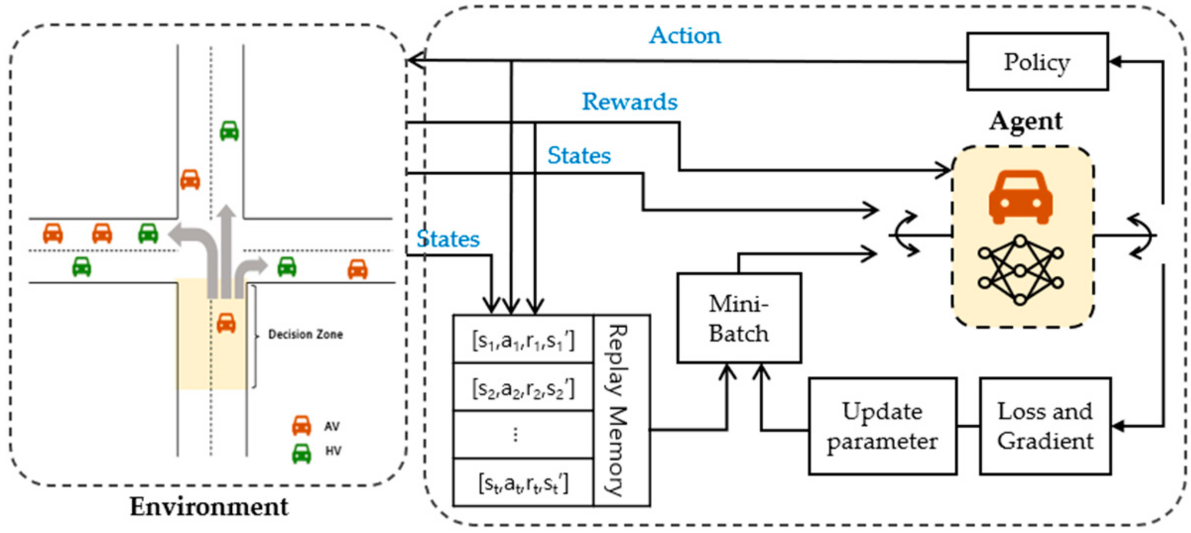
The proposed method recognizes the traffic situation and determines the direction to optimize the route based on the traffic situation. Traffic environments are dynamic and complex, with traffic volumes changing in real time. Consequently, the routes of vehicles are constantly changing and difficult to predict. This is especially the case in mixed traffic environments, the continuous variation due to various factors leads to a high likelihood of many possible states occurring. To address this, we utilized DQN, which is capable of learning complex patterns and interactions in state and action spaces by using neural networks. Additionally, DQN utilizes experience replay to efficiently utilize past experiences in training, thereby enabling the effective utilization of training data and ensuring stable learning even in high-dimensional state and action spaces. Furthermore, DQN is well suited for discrete action spaces, thus making it suitable for determining discrete actions such as driving directions.

The proposed method updates the routes to alleviate traffic congestion by distributing the driving directions based on real-time local information at each intersection. Each AV is considered a DRL agent and is defined by $v\in \left\{v_1,v_2,\dots ,v_n\right\}$, which allows the AVs to interact with the environment and learn the policies to reach their destination. The goal of each AV agent is to drive in a direction that changes toward the destination as quickly and optimally as possible to achieve higher rewards.

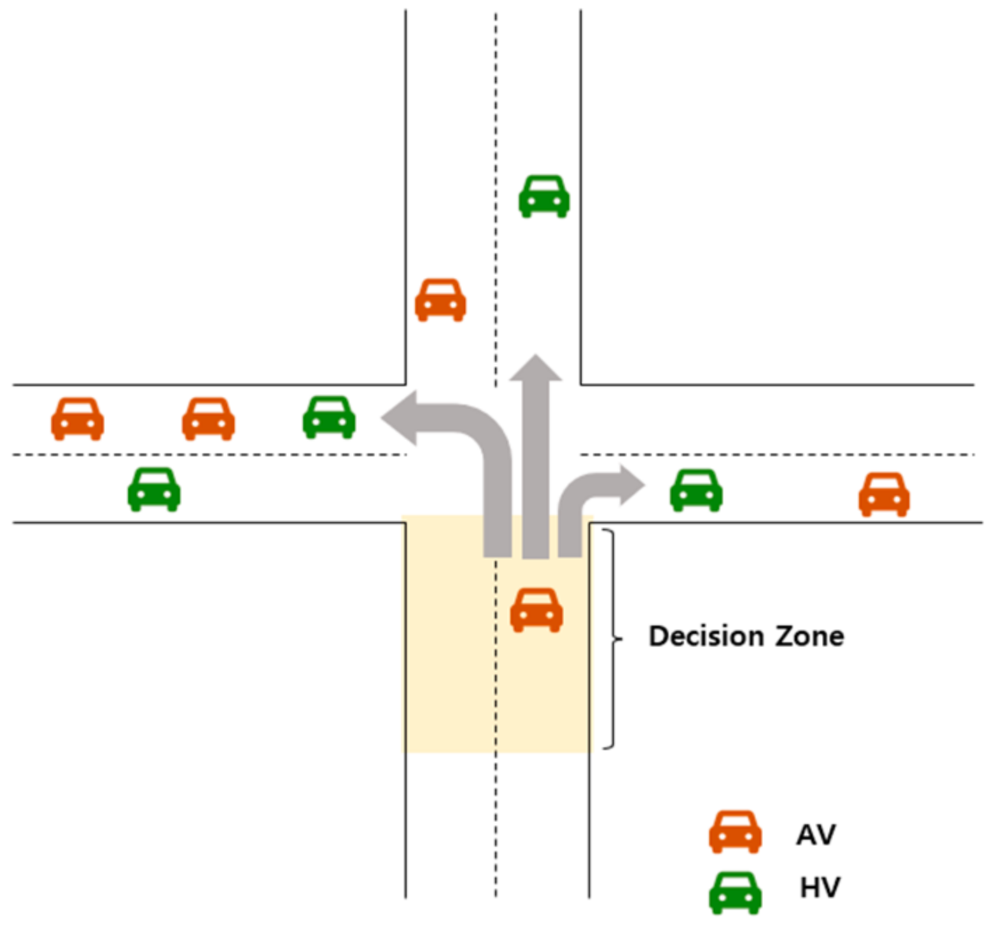
As shown in Figure 1, a decision zone with a specified distance was defined on the approach roads of each intersection. Within these zones, the driving direction of the AV at the intersection was determined. Therefore, when an AV is in the decision zone, it derives the observed state $s_n$ from the current traffic situation to form state space $S$. State $s_n$ is entered into AV agent $v_n$, which represents the current traffic observation. Subsequently, AV agent $v_n$ performs action $a_n$ based on the current state $s_n$. Thereafter, the AV agent receives the reward $r_n$ from the traffic environment. There were three components in the MDP. These comprised a set of states $S$, a set of actions $A$, and an immediate reward $r$, and they were defined as described below.

3.1. State

To control the driving direction of AVs at intersections for distributing traffic flow, state $s_n$ was defined as an efficient representation of the current traffic conditions. The expression variables describe the complexity of the dynamics and include several variables reflecting the mixed traffic environment. The state $s_n$ observed by each AV agent $v_n$ is defined as a matrix $N_r\times \mathcal{F}$, where $N_r$ is the number of nearby roads and $\mathcal{F}$ is the number of features, which is used to represent the current traffic conditions. It includes $p_{n,r}^{AV}$ and $p_{n,r}^{HV}$ (which are the average driving speeds of AVs and HVs), and $m_{n,r}^{AV}$ and $m_{n,r}^{HV}$ (which are the numbers of AVs and HVs driving on road $e$). Moreover, it includes the longitudinal position and lateral position of the current and destination for the AV agent, and these are represented as $l_n^{cur}$ and $l_n^{dest}$. The state $s_n$ is defined in Equation (2):

$$s_n=\left[p_{n,r}^{AV}, p_{n,r}^{HV}, m_{n,r}^{AV}, m_{n,r}^{HV}, l_n^{cur},l_n^{dest}\right].$$

(2)

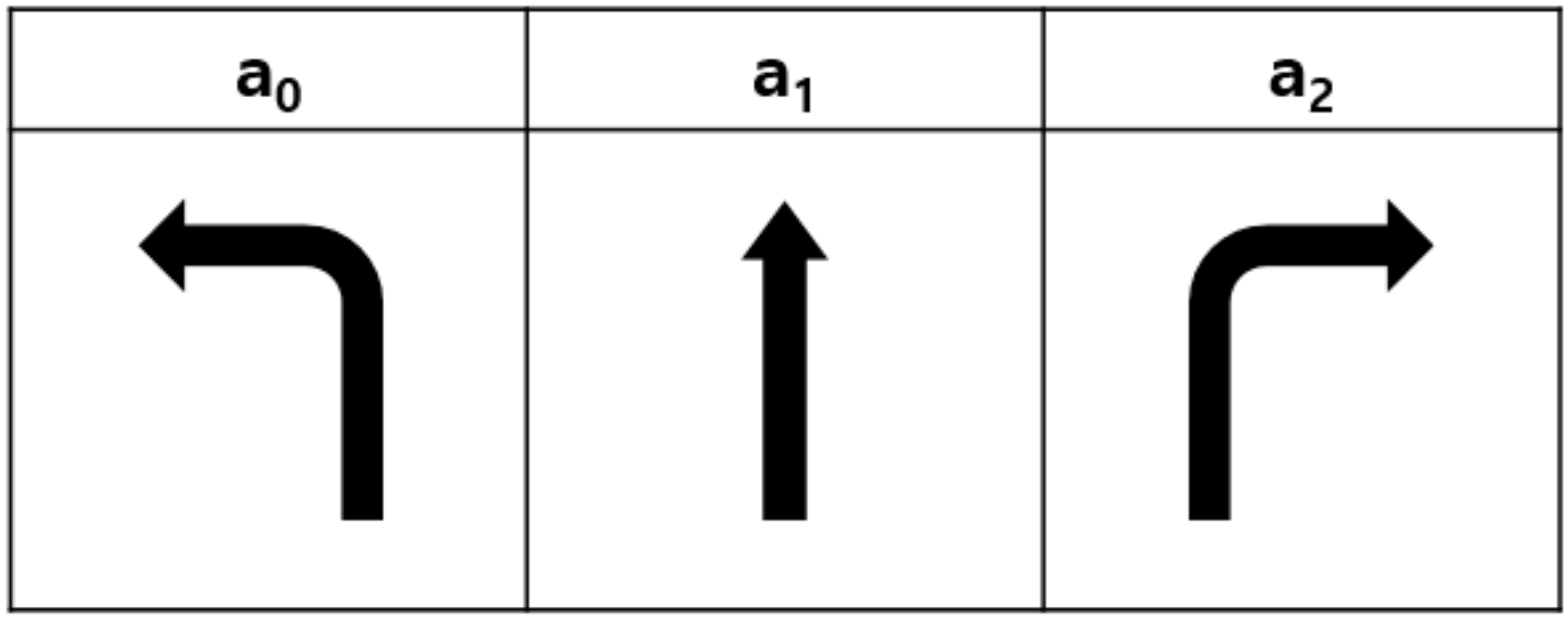
3.2. Action

The action $a_n$ of the AV agent represents a set of driving directions at the intersection, including a left turn, a right turn, or a straight one, and it is determined in the decision zone based on the observed state $s_n$. However, the set of action is dependent on the structure of the considered intersections. In this paper, we considered four-way intersections, thus the possible directions are shown in Figure 2 and Equation (3).

$$a_n=\left[a_0,a_1,a_2\right],$$

(3)

3.3. Reward

The proposed method distributes traffic flow by allowing each AV to reach its destination quickly and efficiently through an optimal control of the driving direction at intersections. It was defined using the objective of the proposed method because the reward function is associated with the objective. Therefore, we designed the reward function to include safety and efficiency.

With the premise of ensuring safety, vehicles should travel at a fast and stable speed; for efficiency, the vehicles should minimize detours to the destination. Therefore, we defined the reward function to maximize the driving speed of the AV $d{s}_n$ and minimize the remaining driving distance to the destination $d{d}_n$. The remaining driving distance is calculated as the sum of the distances between the location of the AV and the destination. The scale of $d{s}_n$ and $d{d}_n$ was normalized to values between 0 and 1. They were then applied as the reward functions due to the following reasons: First, the driving speed incorporates the information on both driving distance and time, with speed being inversely proportional to both driving time and waiting time. Second, considering shorter driving distances helps in reducing the number of AV detours to the destination. Therefore, the reward was defined as given in Equation (3):

$$r_n=\omega ·d{s}_n-\left(1-\omega \right)·d{d}_n,$$

(4)

where $\omega$ is a weighted parameter that adjusts the weight of the driving speed and distance. An algorithm-based DQN is shown in Algorithm 1 and Figure 3.

Algorithm 1. DQN-based vehicle routing control method

Initialize main network $Q(s,a|\theta )$ Initialize target network $Q(s,a|{\theta }^{\prime })$ with weights ${\theta }^{\prime }=\theta$ Initialize the experience replay buffer $\mathcal{D}$ for each episode do   Initialize environment and state $s_n$ for each AV agent $n\in N$   for each agent $n\in N$ do  if agent $n$ in decision zone:    if random number $\le$ $ϵ$:     Select action $a_n$ randomly    else:     Select action $a_n=\mathit{arg}\underset{a}{\max }Q\left(s,a;\theta \right)$    Execute the action $a_n$ and receive reward $r_n$    Store $(s_n, a_n,r_n,{s_n}^{\prime })$ in $\mathcal{D}$    Randomly sample a mini batch of samples from $\mathcal{D}$    Set $y=\left\{\begin{array}{c}r if episode termiates\\ r+\gamma \underset{a^{\prime }}{max} Q\left(s^{\prime },a^{\prime }|{\theta }^{\prime }\right) otherwise\end{array}\right.$    Update $\theta$ with gradient descent step via (1)    Regularly update ${\theta }^{\prime }=\theta$

4. Performance Evaluation

We compared the performance of the proposed method with those of other methods. The simulation was conducted using Python, PyTorch, and simulation of urban mobility (SUMO) [24].

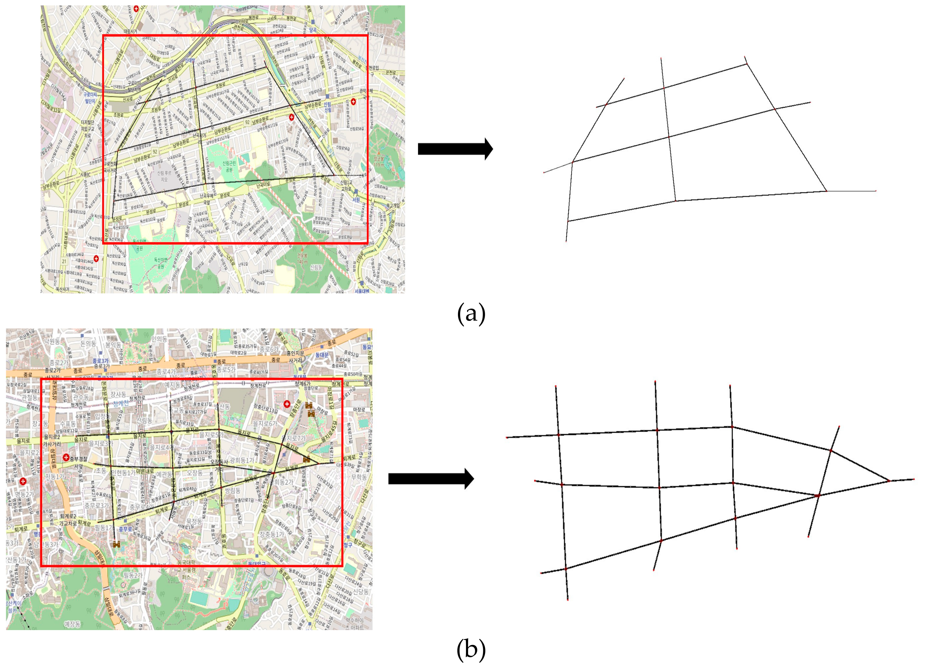
We conducted an experiment with the maps of City1 and City2, which were generated using SUMO, as shown in Figure 4. These two cities were extracted from major roads in parts of Seoul to help with considering real urban traffic environments. The length of the road was at a minimum of 150 m and a maximum of 500 m. The figures on the left in Figure 4a,b show photographs of the considered city, and those on the right show photographs of the edge of the road on the map. Figure 4a shows a simple scenario with fewer edges and intersections. This environment had fewer intersections; thus, there were fewer decision zones. As the edges were long and the number of edges was small, fewer environmental factors were required to be considered. Therefore, it was less dynamic because the number of variables was reduced. Figure 4b shows a complex scenario with many edges and intersections. Compared with the simple scenario, this environment was very dynamic because of the shorter edge length, several decision zones, and numerous variables. In each scenario, traffic conditions with different MPRs and traffic densities were used to test the proposed method.

The origin and destination of AVs and HVs were randomly set on the edge road of the map. The AVs and HVs were distributed according to a Poisson distribution with different maximum initial speeds of $15 \mathrm{m}/\mathrm{s}$. The motion of the HVs followed the Intelligent Driver Model (IDM) [25], where the maximum deceleration and acceleration for safety purposes was limited to $5 \mathrm{m}/\mathrm{s}$, and the politeness factor was $0$. To evaluate the effectiveness of the proposed method, various vehicle arrival rates that corresponded to vehicle density and MPR values, which themselves corresponded with a mixed ratio of AVs and HVs, were used.

The proposed method uses DQN, which consists of the following. The neural network of DQN has four fully connected layers: an input layer, two hidden layers, and an output layer. The first and second hidden layers had 150 and 100 neurons, respectively. A Rectified Linear Unit (RELU) activation function was used for both hidden layers. The ReLU function, defined as $ReLU\left(x\right)=max\left(0,x\right)$, is one of the most widely used nonlinear activation functions for RL. The remaining parameters used in the simulations are listed in

Table 1. List of the hyperparameters.

Parameters	Value
Number of episodes	500
Batch size	32
Learning rate	0.001
$\mathrm{Replay} \mathrm{memory} \mathrm{size} (\mathcal{D})$	10,000
$\mathrm{Discount} \mathrm{factor} \mathrm{of} \mathrm{long}\text{-}\mathrm{term} \mathrm{reward} (\gamma )$	0.99
$\mathrm{Exploration} (ϵ)$	$1\to 0.01$

.

To evaluate the performance of the Proposed method, we leveraged two methods with the reward parameters [20], which are defined as follows: the combination of driving speed and accumulated driving distance (ds + ad), and the combination of driving speed and the number of vehicles on the road (ds + nv). The method proposed in [19] is referred to as Compare, where a reward function was designed with a single objective focusing on driving time.

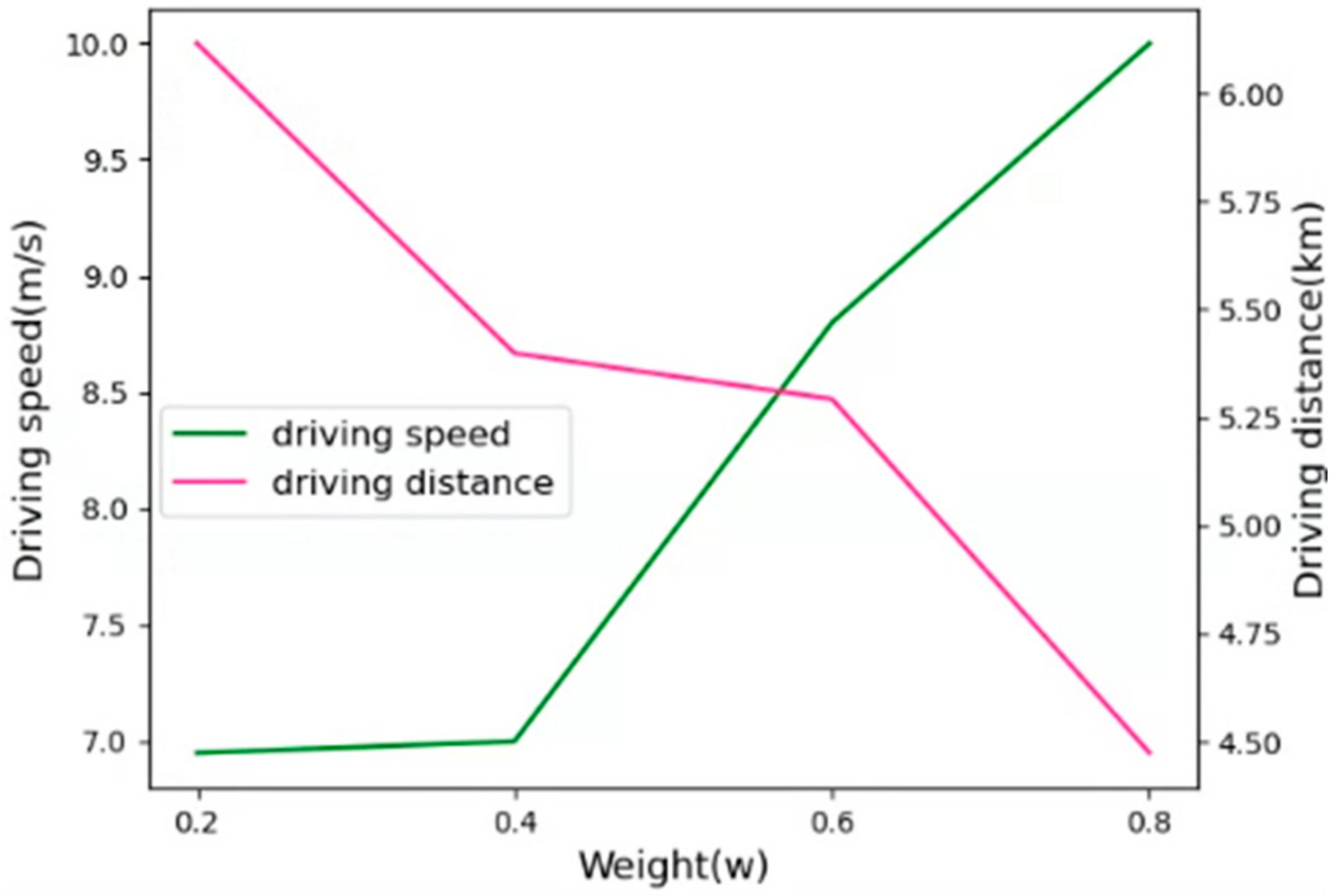
Figure 5 shows the effect of weights $\omega$ on the performance. The weight parameter $\omega$ was used as the strategic parameter of the reward function, which resulted in a tradeoff between the driving speed and distance of the AVs. To determine the optimal weight $\omega$ for the driving speed and distance, we evaluated the performance by varying the weight $\omega$. In the following simulations, we set weight $\omega$ to 0.6, which focused slightly more on the driving speed.

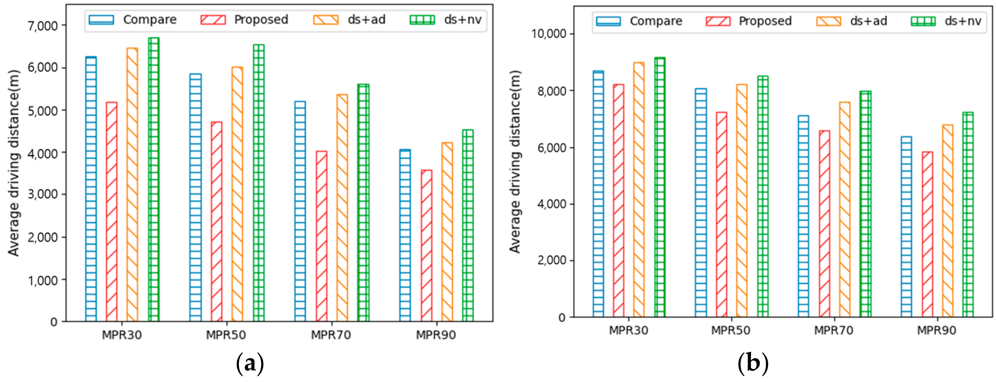
Figure 6a,b show the average driving distance for AVs to reach their destinations under different MPRs in City1 and City2, respectively. The MPR values are 30%, 50%, 70%, and 90%, thus indicating the ratio of AVs in a mixed traffic environment. For instance, MPR 90 comprises 90% AVs and 10% HVs in a traffic environment. The AVs learn to optimize their routes to the destination depending on the traffic situation; the higher the MPR, the lower the driving distance of the AVs. Therefore, as the MPR increases, the number of AVs learning the optimal route increases, thereby decreasing the driving distance to the destination. It is evident that the performance difference between City1 and City2 was relatively small. This was because it was less dynamic due to the fewer intersections and decision zones.

Proposed yields increased the values in the approximate range of 12–25% in City1 and 7–15% in City2 in terms of the driving distance when compared with those of Compare and ds + ad. This was because the number of detours decreased when the remaining driving distance from the destination was considered. The reward model of Compare is expressed in driving time, whereas the reward model of ds + ad is in terms of driving speed and accumulated driving distance. Therefore, Compare and ds + ad are more likely to detour because they choose a shorter driving time and distance, regardless of the distance to the destination, when determining the route. In addition, the rewards for both Compare and ds + ad include information on the driving time; however, the expressions for the reward are slightly different. Compare is a single reward and ds + ad is a combination of driving time and distance. These have different weights for the driving speed and distance. Compare balances the driving speed and distances, whereas ds + ad is more focused on driving speed than on driving distance. Therefore, ds + ad drives approximately 3–7% more of a distance than Compare in City1 and City2. Furthermore, ds + nv exhibited the worst performance in terms of driving distance. This is because the ds + nv model has more detour routes than other methods as its model rewards driving speed and vehicle density without considering the driving distance.

Table 2. Average driving speed in City1 and City2 (unit: m/s).

	Compare	Proposed	ds + ad	ds + nv
City1	7.29 ± 0.13	7.55 ± 0.11	7.31 ± 0.14	7.18 ± 0.13
City2	8.44 ± 0.19	8.89 ± 0.22	8.66 ± 0.25	8.3 ± 0.19

presents the average driving speeds at which the AVs traveled to their destination in City1 and City2. Compare attempted to drive quickly to minimize travel time, while the other three methods aimed to reduce the driving distance or vehicle density while maintaining a high speed. This meant that all four methods had information about the driving speed; thus, the performance difference was relatively small, i.e., about 1–6% in City1 and City2. The driving speed also increased as the MPR increased. This was because multiple AVs learn to drive along the optimal route based on traffic conditions. Despite City1 having a smaller scale, its AV speed is approximately 13–15% slower than that of City2 due to the higher vehicle density on its roads.

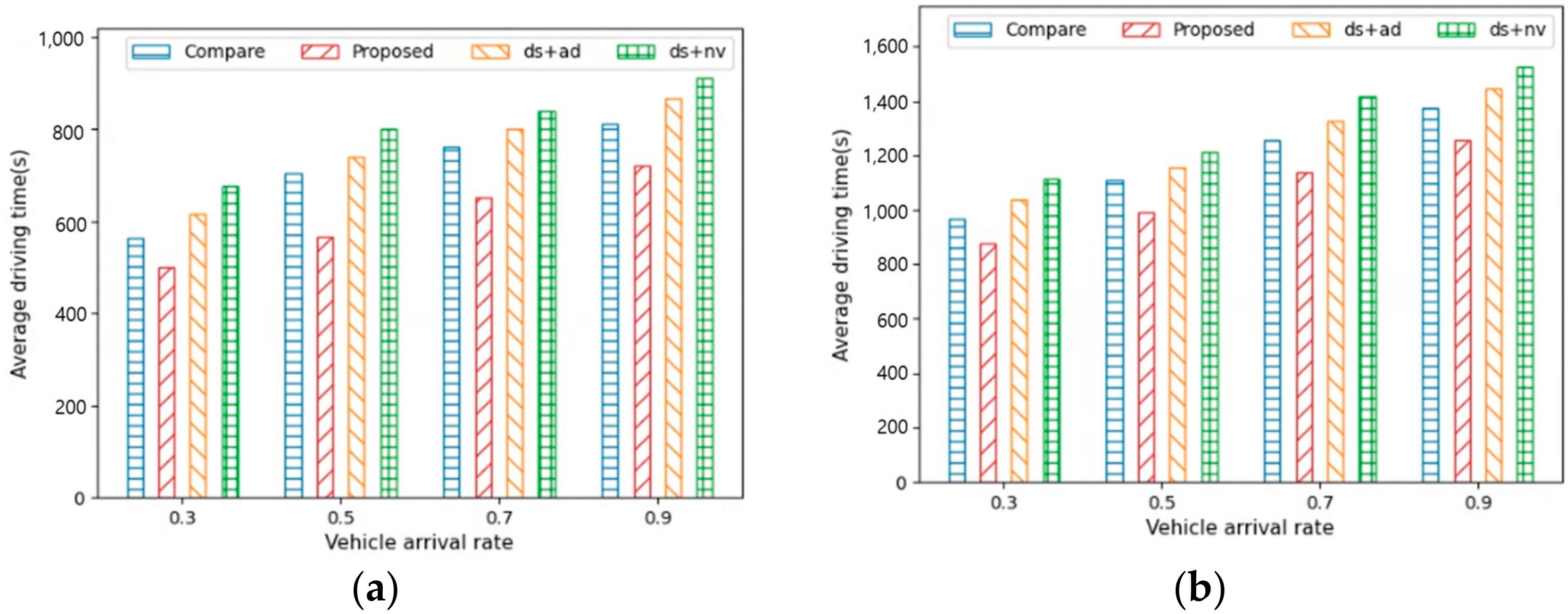
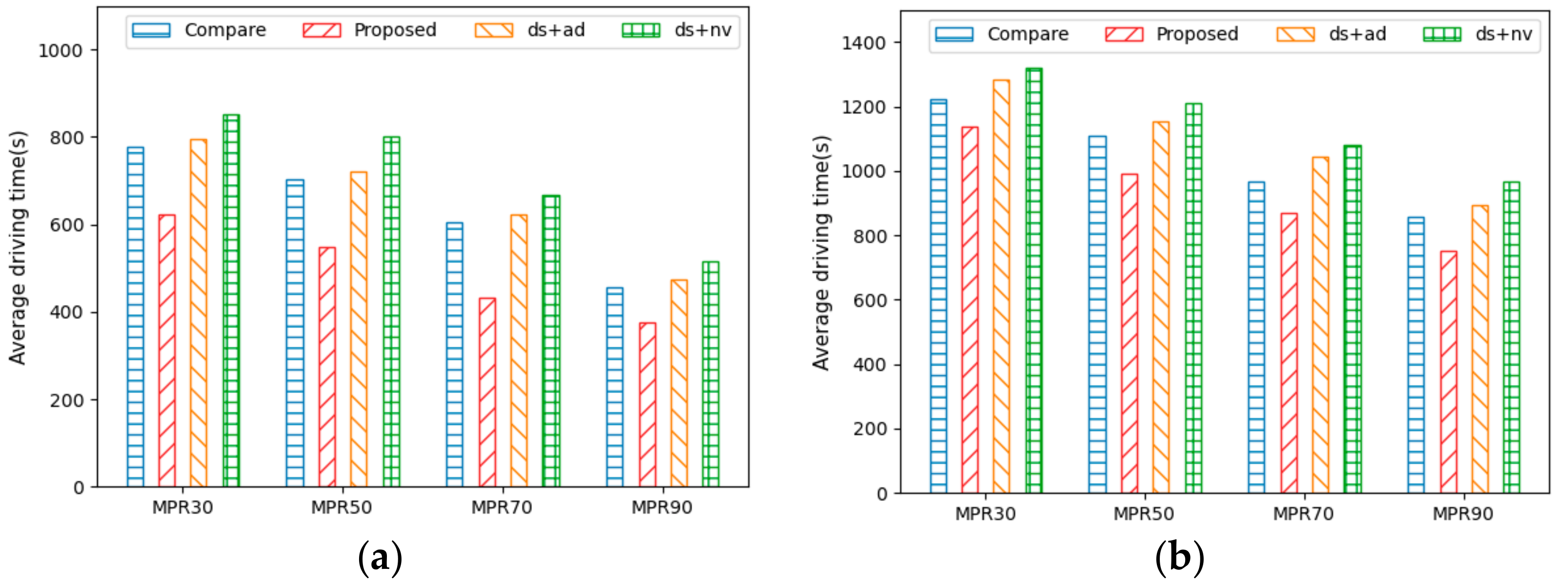
Figure 7a,b show the average driving time for AVs to reach their destinations under different MPRs in City1 and City2. The figures illustrate that the driving time decreases as the MPR increases. This indicates that the higher the number of AVs, the better the traffic flow. Additionally, the driving time is affected by both distance and speed, with shorter distances and higher speeds resulting in shorter driving times. Therefore, Proposed, which performed best in terms of both driving distance and speed, showed performance improvements of about 18–28% in City1 and 7–17% in City2 when compared with those of the other methods. Moreover, due to fewer detours on the way to the destination, Proposed was more efficient in terms of distance, thereby leading to shorter travel times. Compare designed its reward by considering only driving time as a single objective, while ds + ad designed its reward by considering travel time as a linear function through which to address multiple objectives. Hence, although both methods aim to minimize travel time, they showed a difference of about 8–10% due to the different reward designs. On the other hand, ds + nv considers only travel speed and vehicle density, thus resulting in many detours to the destination due to the lack of consideration for driving distance. Consequently, it exhibited the worst performance in terms of travel distance, thereby leading to a lower travel time performance compared to other methods.

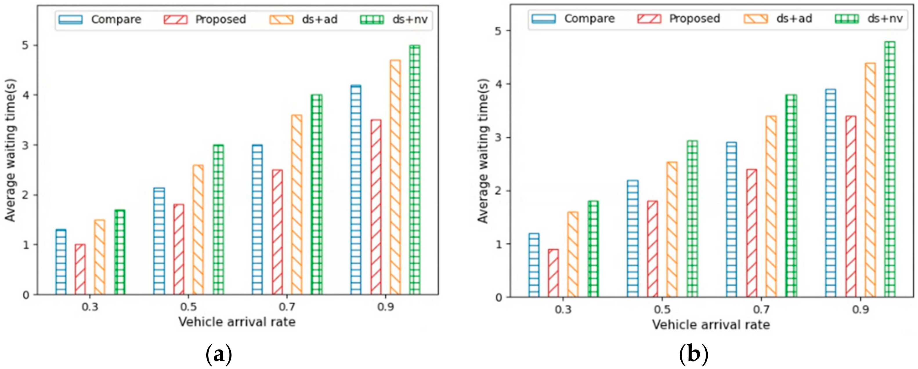
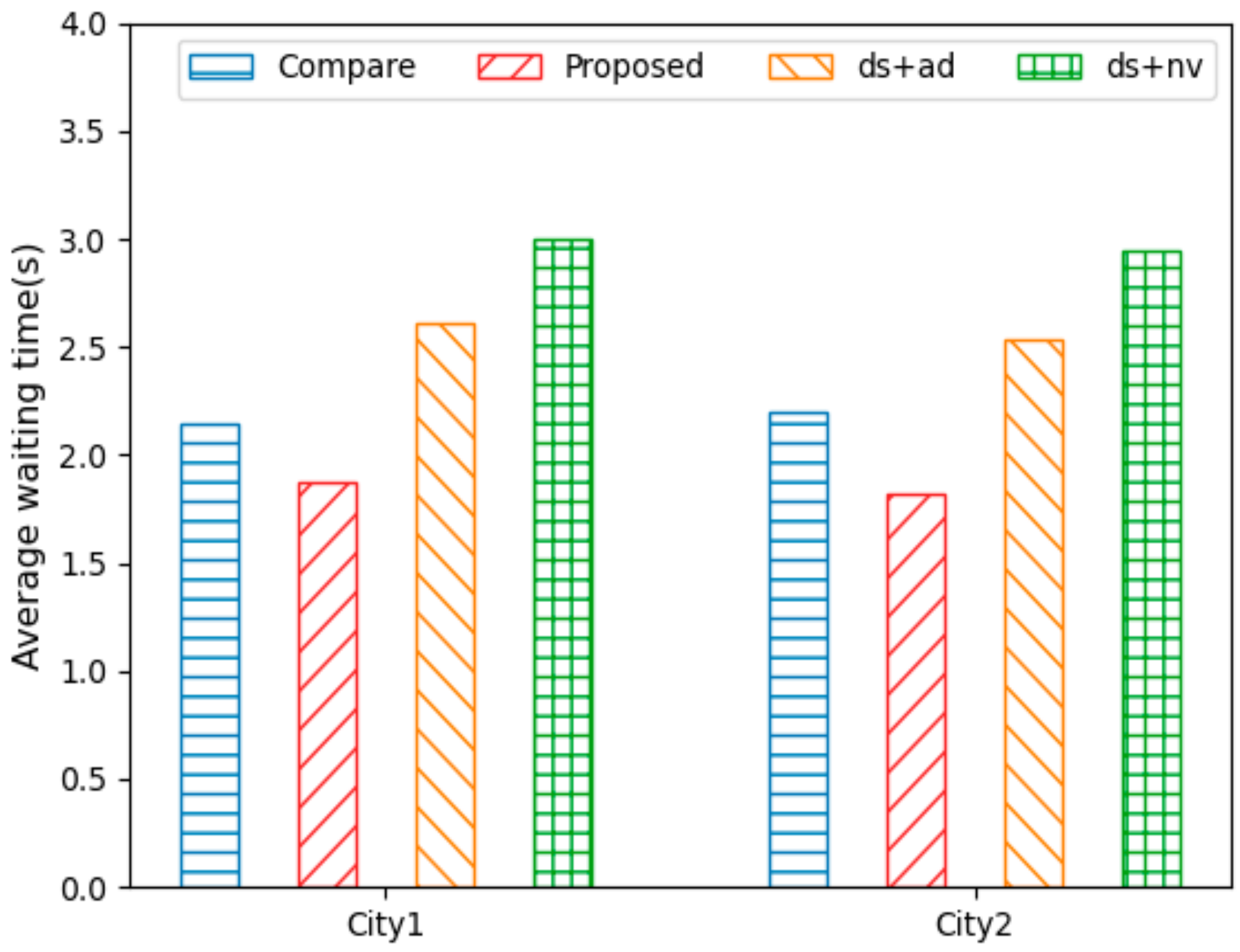
Figure 8 shows the average waiting times for AVs in City1 and City2. A low average waiting time implies that the traffic flows smoothly and that the AVs drive without waiting. It can be observed that Proposed had a shorter waiting time than the other methods. Therefore, Proposed indicated a better distribution of traffic flow than the other methods. As mentioned previously, as the MPR increases, the driving distance and driving time of the AVs decrease, and the driving speed of the AVs thus increases. In other words, the higher the ratio of AVs adapted to the dynamic environment, the smoother the traffic flow, and the lower the waiting time of the AVs. In addition, the reduction in the waiting time for the AVs indicated that the traffic congestion was low and had a good distribution, thereby implying that the density of AVs was minimized. Therefore, City1, with its higher vehicle density, exhibited approximately 13–15% longer waiting times than City2.

Figure 9a,b show the average driving time for AVs to reach their destinations under different vehicle arrival rates in City1 and City2. Figure 10a,b show the average waiting time for AVs under different vehicle arrival rates in City1 and City2. The figures indicate that the average driving and waiting times when the vehicle arrival rates (where the MPR value was 50%) were 0.3, 0.5, 0.7, and 0.9. As the vehicle arrival rate increased, the number of vehicles on the road also increased. This led to higher traffic density on the roads, thus resulting in increased traffic congestion. Consequently, the driving and waiting times for the AVs in City1 and City2 increased. Proposed, which minimizes detour routes to the destination, exhibited the best performance in terms of average driving and waiting times. This was because Proposed ensures smooth traffic flow regardless of the vehicle arrival rate. Compare and ds + ad, which have relatively few detours, then followed, and ds + nv was found to deliver the worst performance due to recommending many detours.

Thus, Proposed yielded the best performance in any environment when the MPR was low or high, as well as when the vehicles were high or low in density. In addition, the performance of Proposed was more pronounced in a more dynamic traffic environment. If the driving distance was simply defined as a reward function without considering the destination, the shortest distance between actions was selected. This generated detours to the destination, which increased both driving time and distance. Consequently, the likelihood of traffic problems, such as traffic congestion, increased. Therefore, Proposed was modeled as a reward function by considering the distance from the current location to the destination. Hence, the detour situation was reduced, thereby resulting in a good performance in terms of the driving distance and increased efficiency. Consequently, the agent learns to drive at high speeds without detours, thus enabling it to perform better in terms of driving time. Moreover, the AVs performed well in terms of waiting time because the traffic flowed smoothly as it traveled along optimal routes. This meant that Proposed distributes traffic flow well, thus alleviating traffic congestion.

5. Conclusions

This study considered a mixed traffic environment with a combination of AVs and HVs. We proposed a DRL-based vehicle routing control method with multiple objectives that incorporate safety and efficiency to distribute traffic flow. Therefore, the objective of this study was to maximize the long-term reward in terms of driving speed and remaining driving distance to the destination by controlling the direction at intersections to distribute traffic flow, as well as to control the routes safely and efficiently to the destination. We described and formulated a dynamic traffic environment as an MDP system. A DQN was adopted for the optimal route control method, and each AV—as an agent—learned its policy independently. We compared the proposed method with conventional methods and other methods through simulations; the simulation results showed that the proposed method minimized the driving distance, time, and waiting time of the AVs in any environment and for all MPRs and traffic densities.

This study has limitations in that each agent learned independently like a single agent, and that the environment used was simple as it considered only four-way intersections. In the future, we will utilize driving behavior data with varying road characteristics and will apply various scenarios [26]. In addition, we will consider that each agent learns in cooperation with others, rather than learning independently, in a dynamic mixed traffic system. Furthermore, we plan to extend the vehicle routing control method based on counterfactual multi-agent policy gradient learning, which determines the contribution of each agent to the overall reward in cooperation with each other.