A Simplified Radiation Characteristic Analysis Method for Defocus-Fed Parabolic Antennas in a W-Band Communication System

Abstract

With increasing interest in the W-band, there is growing focus on parabolic reflector antennas that are known for efficiently inducing high-gain radiation characteristics. There is particular focus on parabolic antennas with diverse defocus-fed applications, including monopulse tracking, multi-beam formation using multiple feeds, and aperture-shared antennas for multi-band operation. Thus, a new simplified method is presented in this paper to analyze the radiation characteristics of defocus-fed parabolic antennas. The presented method is based on the discrete division of a parabolic reflector surface and considers only simplified wave propagation theory and the effect of the scalar function pattern from the feeder. Additionally, array theory is exclusively applied for the analysis of radiation characteristics. Therefore, the presented method uses a very simplified formula to calculate the radiation characteristics of a defocused parabolic reflector antenna. The performance of the presented method was evaluated by comparing the results with commercial EM tools. The results of the analysis confirm the applicability of the presented method for the analysis of defocus-fed parabolic antennas.

1. Introduction

Applications of high-speed and broadband communication services are expected to broaden across diverse frequency bands as a result of the surge in information volume driving an increase in demand. The W-band (75 GHz to 110 GHz) stands out as a prospective candidate for sub-terahertz communications in sixth-generation mobile communications, along with its applications in radar systems, automobile collision avoidance systems, and image sensing [1,2,3]. The W-band, distinguished by the short wavelength inherent to millimeter waves, is able to facilitate compact hardware implementation for the propagation of electromagnetic waves. However, it is accompanied by drawbacks such as atmospheric attenuation and high path loss due to its short wavelength. An antenna system with enhanced radiation characteristics (high gain) becomes essential to overcome these limitations [4].

The subsequent studies serve as examples of W-band high-gain radiation characteristics. A modular array antenna for an electron cyclotron emission imaging system [5], a substrate-integrated waveguide (SIW) for microwave power transmission (MPT) and wireless communications [6], and a folded Fresnel reflector (FFR) for a helicopter collision avoidance radar and a microstrip patch array antenna fed by SIW for an operating range from 91 GHz to 97 GHz [7] were all previously designed and studied. The mentioned antennas use dielectrics. As the operating frequency increases, dielectric loss increases, and thus antenna radiation efficiency decreases. In addition, these antennas belong to the category of resonant antennas; they suffer from the drawback of having a narrow operating bandwidth.

A parabolic reflector antenna has the benefits of providing high gain, radiation efficiency, and wide bandwidth compared to the other types of antennas. Therefore, a parabolic reflector antenna is a good candidate for W-band applications. In Refs. [8,9], parabolic antennas were designed and studied for W-band satellite communication (SATCOM) applications. Parabolic reflector antennas can be used in more diverse ways in addition to inducing high-gain radiation characteristics for the W-band. In Ref. [10], a monopulse tracking system was designed based on a parabolic antenna for W-band wireless communications. In Ref. [11], W-band multi-beam antenna systems and millimeter-wave image systems were designed with multi-fed parabolic reflector antennas. In Ref. [12], a multi-band shared aperture reflector antenna was designed for the Ka- and W-bands.

It is also necessary to be able to analyze the radiation characteristics of the defocus-fed parabolic reflector antenna for the various mentioned applications. Electromagnetic field analysis is necessary for analyzing the radiation characteristics of antennas. For this purpose, various efficient methods have been developed to simulate an electromagnetic field. Representative methods include the method of moment (MOM) [13], the finite element method (FEM) [14], the finite difference time domain (FDTD) [15], the finite difference method (FDM) [16], and the finite integration technique (FIT) [17].

However, in a high-frequency regime or with electrically large objects such as reflector antennas, the computational burden associated with the mentioned methods is prohibitively high. Therefore, high-frequency asymptotic methods, such as geometrical optics (GO) [18,19] or physical optics (PO) [20,21,22,23], have been extensively applied to solve approximate solutions for reflector antennas with a limited computing cost while maintaining good accuracy. The GO method is based on the description of an electromagnetic field in terms of optical rays. It focuses on the reflection of rays as they interact with the parabolic surface and is commonly used to predict the path and concentration of electromagnetic energy in large-scale antenna structures. The PO method considers electromagnetic waves as a combination of incident and scattered fields based on the equivalent currents on the surface. It involves evaluating the contributions from both direct and reflected paths, considering the physical characteristics of the reflecting surface. GO and PO methods have also been extended to the geometrical theory of diffraction (GTD) and physical theory of diffraction (PTD) by explicitly incorporating diffraction phenomena to enhance analytical accuracy [24,25,26].

However, these methods require analyses of the electric field integral equation (EFIE) or magnetic field integral equation (MFIE), the induced current distributions on surfaces, ray tracing, the reflection/refraction/diffraction phenomena of electromagnetic waves, boundary conditions, etc.

This paper presents a simple method for analyzing the radiation characteristics of a defocus-fed parabolic antenna in high-frequency regimes. The presented method is a simplified approach to the PO technique and refers to the analysis of antennas using discrete components studied in [27,28,29]. The presented method is based on the discrete division of a parabolic reflector surface and considers only simplified wave propagation theory and the effect of the scalar function pattern from the feeder. Additionally, array theory is exclusively applied for the analysis of radiation characteristics. Therefore, a very simplified formula is used to calculate the radiation characteristics of a defocused parabolic reflector antenna. The performance of the presented simplified method was validated by comparing its results with those obtained from two representative commercial tools: GRASP (General Reflector Antenna Design Software Package) and CST (Computer Simulation Technology) Studio Suite. These tools utilize PO/GTD and FIT techniques, respectively. The validation process covered a range of configurations for defocus-fed parabolic antennas. The details of the presented method and its validation through simulation experiments are discussed in the following sections.

2. Parabolic Antenna Analysis Method

The presented method for analyzing the radiation characteristics of a defocus-fed parabolic reflector antenna consists of the following procedures: discretizing the parabolic reflector surface, substituting each division point with point charge sources, considering the influence of the feed and wave propagation paths from each point charge source, and incorporating the influence of the feed pattern.

In the discrete division procedure of the reflector surface, both the presented method and previous research methods (PO, etc. [18,19,20,21,22,23]) discretely divide the reflector surface. However, the difference lies in the purpose of this discretization. In existing research methods, discrete division is performed to calculate the reflector surface using numerical integration methods (mensuration by parts). Comparatively, the presented method discretizes the reflector surface with the specific purpose of replacing it with point charge sources (sampling). Therefore, there is a difference in the objective of discretization, and this difference also leads to simplified computations in the presented method.

The radiation characteristics of a reflector antenna require the calculation of radiated electric fields based on the induced currents on the reflector surface. To achieve this, in previous research [20,21,22,23], it was necessary to calculate the current distribution on the discretely divided reflector surface using methods such as EFIE or MFIE. However, in the presented method, since the reflector is discretely divided and replaced with point charge sources, it is only necessary to consider the amplitude and phase effects based on the wave propagation paths depending on the location of the point charge sources. Therefore, the presented method simplifies the process of calculating the electric field effects for the radiation characteristics of the reflector antenna.

The influence of the feed pattern also needs to be considered in the calculation of the radiation characteristics of a reflector antenna. In previous research [18,19,20,21,22,23], the influence of the feed pattern was accounted for using vector functions. However, in the presented method, only scalar functions are considered, leading to further simplification of the formulas.

In previous research, it was necessary to integrate the entire electric field distribution based on the feed pattern and the current distribution on the reflector surface to calculate the radiation characteristics [20,21,22,23]. However, in the presented method, only the effects of discretely distributed point charge sources are considered, allowing for the calculation of radiation characteristics based on array theory. Array theory is used to calculate the radiation characteristics of discretely distributed radiating elements, and it involves simple summation operations instead of integration. This leads to the simplification of the formulas.

2.1. Parabolic Reflector Surface Division

The procedure of parabolic reflector surface division is as follows, where, for the configuration of a parabolic antenna, the focal point is established as the origin of the coordinate system and the aperture plane is defined in the x-y plane:

• Considering the x-z plane as a reference, the parabolic curve is uniformly divided at equidistant intervals, and the calculation of ${\psi }_i$ is based on this division.
• Considering each ${\psi }_i$ as a reference for the uniform division of the parabolic surface’s circumference, the calculation of ${\varphi }_S^i$ is based on circumference division.

Figure 1 shows a conceptual diagram of the procedure for parabolic reflector surface division.

The Cartesian coordinates $\left(x, z\right)$ corresponding to ${\psi }_i$ for step #1 of the parabolic reflector surface division procedure are given by Equation (1). This is derived based on the formula in [30] for analyzing the structure of a typical parabolic reflector antenna.

$$(x_i, z_i)=\left(\frac{F}{{\cos }^2\left({\psi }_i/2\right)}\sin \left({\psi }_i\right) , -\frac{F}{{\cos }^2\left({\psi }_i/2\right)}\cos \left({\psi }_i\right)\right)$$

(1)

where $F$ is the focal length of the parabolic reflector.

Let the position vector of the $i$-th division point be denoted $\overrightarrow{r_i}$, according to Equation (1); assuming a required uniform division interval of $g_{\psi }$, ${\psi }_i$ can be determined by satisfying the condition given in Equation (2).

$$\left|\overrightarrow{r_i}-\overrightarrow{r_{i+1}}\right|\approx g_{\psi }$$

(2)

where the value ${\psi }_1$ required to determine the position vector $\overrightarrow{r_1}$ is given by the maximum angle for the parabolic reflector configuration, which is $2 \mathit{arctan}\left(0.25 D/F\right)$, in which $D$ is the diameter of the parabolic aperture. As $i$ increases, $\psi$ gradually decreases until it reaches 0$°$.

Step #2 of the parabolic division procedure involves dividing a circumference on the parabolic surface at equidistant intervals, determined by ${\psi }_i$. When the required interval is $g_{\varphi }$, the value of ${{\varphi }_s}^i$ resulting from equidistant division with respect to ${\psi }_i$ can be obtained using Equations (3) and (4).

$${{\varphi }_s}^i=2\pi x_i / M^i$$

(3)

$$M^i=round\left(2\pi x_i/g_{\varphi }\right)$$

(4)

where $x_i$ is calculated with Equation (1), and $round\left( \right)$ represents the rounding function.

In this paper, a parabolic reflector surface is divided and the resulting points are replaced with charge point sources for the purpose of analyzing the radiation characteristics of a parabolic antenna. Therefore, the positions of each charge point source resulting from the parabolic reflector surface division procedure can be defined through the following equations:

$$P_{\left(i,j\right)}^x=R_i\sin \left(\pi -{\psi }_i\right) \cos \left({{\varphi }_s}^{i}j\right)$$

(5)

$$P_{\left(i,j\right)}^y=R_i\sin \left(\pi -{\psi }_i\right) \sin \left({{\varphi }_s}^{i}j\right)$$

(6)

$$P_{\left(i,j\right)}^z=R_i\cos \left(\pi -{\psi }_i\right)$$

(7)

where $j$ is an integer satisfying $0\le j\le M^i$.

The positions of the point sources according to Equations (5)–(7) form a ragged matrix. For the convenience of analysis, flattening the matrix yields the following equations:

$$P_n^x=R_n\sin \left({\theta }_n\right) \cos ({\varphi }_n)$$

(8)

$$P_n^y=R_n\sin \left({\theta }_n\right) \sin \left({\varphi }_n\right)$$

(9)

$$P_n^z=R_n\cos \left({\theta }_n\right)$$

(10)

where $n$ is a natural number satisfying $1 \le n \le N$, in which $N$ is equal to $\sum M^i$.

Figure 2 shows the results of the presented parabolic reflector surface division procedure based on $\left(g_{\psi }, g_{\varphi }\right)$ = (0.5$\lambda$, 0.5$\lambda$) and (1.0$\lambda$, 1.0$\lambda )$. Here, D is set to 30$\lambda$, and the FD ratio ($F/D$) is set to 0.35.

2.2. Induced Amplitude Calculation

In a parabolic reflector surface replaced by charge point sources, each charge point source is influenced by the radiated electromagnetic waves from the feeder, resulting in induced signals. In this paper, we derived the amplitudes of the induced signals for each charge point source based on such influences. Here, the impact from the feeder is considered using only scalar functions, and the electromagnetic field theory for induced signal analysis is simplified.

The amplitude of induced signals is divided into two categories. The first is the influence of the electric field intensity due to wave propagation from the feeder, and the second is the influence of the radiation pattern of the feeder.

In the electric field integral equation (EFIE) [31] used to determine the electric field intensity at observation positions (the positions of each charge point source) resulting from wave propagation from the feeder, the electric field intensity based on the far-field approximation is inversely proportional to the distance between the feeder and the observation point. In this paper, relying on this phenomenon, we took the decrease in electric field intensity at each charge point source location as the first induced signal amplitude. Therefore, the induced signal amplitude due to wave propagation from the feeder is defined as in Equation (11).

$$I_n^{ R}=\frac{1}{\left|\overrightarrow{r_f}-\overrightarrow{r_n}\right|}$$

(11)

where $\overrightarrow{r_f}$ is a position vector according to the position $\left(f_x, f_y, f_z\right)$ of the feeder, and $\overrightarrow{r_n}$ is a position vector according to the position $\left(P_n^x , P_n^y , P_n^z\right)$ of the $n$-th charge point source.

Generally, the feeder of a parabolic reflector antenna is composed of a horn antenna, which exhibits a directional radiation pattern. Therefore, the electric field intensity at each charge point source is influenced by the radiation pattern of the feeder. The amplitude of the induced signal at each charge point source can be defined as in Equation (12), where the radiation pattern of the feeder is assumed by the cosine-q model [32] and the angle between the beam axis of the feeder and each point source is denoted by ${\mathsf{\Theta }}_n$.

$$I_n^{ P}={\cos }^q\left({\mathsf{\Theta }}_n\right)$$

(12)

For a defocus-fed parabolic antenna, not only is the position of the feed axis displaced, but the beam axis may also not steer toward the center of the reflector. Therefore, in calculating ${\mathsf{\Theta }}_n$ in Equation (12), the position $\left(f_x, f_y, f_z\right)$ of the feeder and the beam steering angle $\left({\theta }_s, {\varphi }_s\right)$ need to be considered. In this paper, considering the influence of the feeder configuration, each charge point source is moved and rotated according to Equation (13), and ${\mathsf{\Theta }}_n$ is calculated based on Equation (14).

$$\left[\begin{array}{c}R{P}_n^x\\ R{P}_n^y\\ R{P}_n^z\end{array}\right]=\left[\begin{array}{ccc}\cos \left(\pi -{\theta }_s\right)\cos \left(-{\varphi }_s\right)& -\cos \left(\pi -{\theta }_s\right)\sin \left(-{\varphi }_s\right)& \sin \left(\pi -{\theta }_s\right)\\ \sin \left(-{\varphi }_s\right)& \cos \left(-{\varphi }_s\right)& 0\\ -\sin \left(\pi -{\theta }_s\right)\cos \left(-{\varphi }_s\right)& \sin \left(\pi -{\theta }_s\right)\sin \left(-{\varphi }_s\right)& \cos \left(\pi -{\theta }_s\right)\end{array}\right]\left[\begin{array}{c}{P}_n^x-f^x\\ P_n^y-f^y\\ P_n^z-f^z\end{array}\right]$$

(13)

$${\mathsf{\Theta }}_n=\frac{\sqrt{{\left(R{P}_n^x\right)}^2+{\left(R{P}_n^y\right)}^2}}{R{P}_n^2}$$

(14)

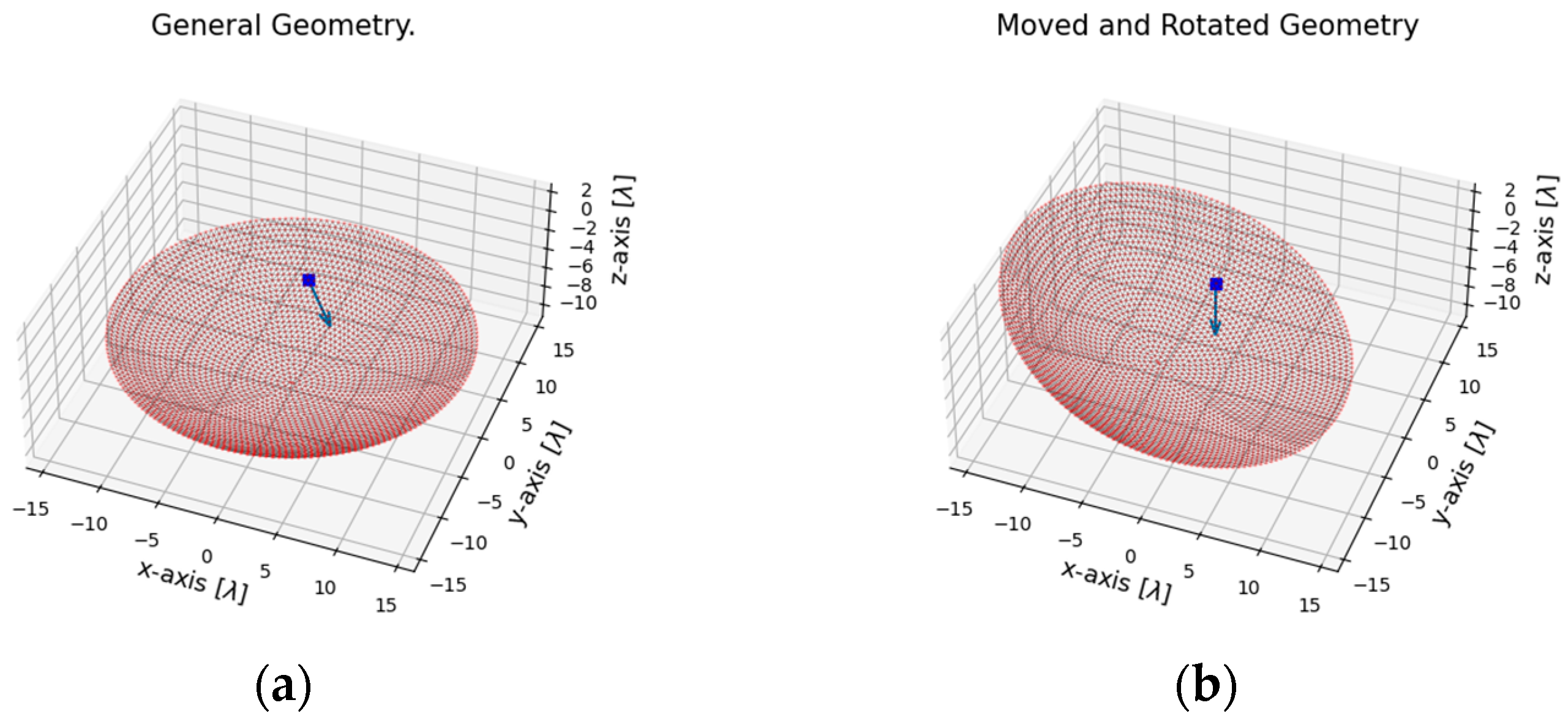
Figure 3 shows the geometry of the divided parabolic reflector surface for $\left(P_n^x , P_n^y , P_n^z\right)$ based on Equations (8)–(10) and $\left(R{P}_n^x, R{P}_n^y, R{P}_n^z\right)$ based on Equation (13). Here, the values of the parameters are specified as follows: D is set to 30$\lambda$, the FD ratio ($F/D$) is set to 0.35, $\left(g_{\psi }, g_{\varphi }\right)$ are set to (0.5$\lambda$, 0.5$\lambda$), $\left(f_x, f_y, f_z\right)$ are set to ($1\lambda$, $1\lambda$, 0), (${\theta }_s$, ${\varphi }_s$) are set to ($160°$, $35°$), and $q$ is set to 1. In Figure 3, the square marker represents the feeder position, and the direction of the arrow indicates the beam axis of the feeder.

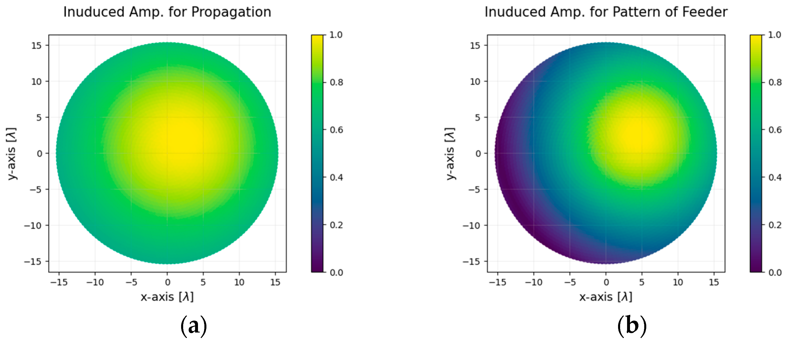
Figure 4 shows the distributions of normalized induced signal amplitudes on the parabolic reflector surface, considering the effects of induced signals due to wave propagation from the feeder and those based on the radiation pattern of the feeder. Here, the antenna configuration is identical to that shown in Figure 3a. Figure 4a displays the amplitude of the induced signals resulting from the electric field effects caused by wave propagation between each point charge source from the feeder. It is evident that the distribution adheres to an inverse distance relationship, as described by Equation (11). Owing to the feeder’s offset $\left(f_x, f_y, f_z\right)$ from the focal position, as presented in Figure 3a, the distribution around the reflector surface is observed to be asymmetrically distributed. Figure 4b illustrates the amplitude of the induced signals for each point charge source due to the feeder’s radiation pattern. The influence of the radiation pattern simulated by the cosine-q model ($q=1$) and the impact of beam steering (${\theta }_s$, ${\varphi }_s$) from the feeder lead to an asymmetric distribution.

2.3. Induced Phase Calculation

In the electric field integral equation (EFIE) [31] used to determine the electric field intensity at observation positions (positions of each charge point source) due to wave propagation from the feeder, the phase of the electric field intensity is related to the distance between the feeder and the observation point. The induced signal phase at each charge point source can be defined using Equation (15), considering the phase values along the propagation path and the boundary conditions on the reflecting surface.

$$a_n=-k\left|\overrightarrow{r_f}-\overrightarrow{r_n}\right|$$

(15)

where $k$ is the wave propagation constant.

Figure 5 illustrates the induced phase distribution on both the parabolic reflector’s surface and the parabolic aperture, as determined using Equation (15). The antenna configuration presented here corresponds to that depicted in Figure 3a. In the induced phase distribution on the parabolic aperture in Figure 5b, the non-uniform distribution arises not only due to the displacement of the feed axis but also due to the possibility that the beam axis may not steer toward the center of the reflector.

2.4. Radiation Characteristic Analysis

In this paper, the parabolic reflector’s surface was divided and replaced with charge point sources. Consequently, the radiation pattern can be derived based on array theory for these charge point sources. The array theory-based radiation pattern [32], as expressed in Equation (16), can be obtained by considering the magnitude and phase of the induced signals, along with the phase differences based on the positions of each charge point source in the far-field region.

$$f\left(\theta , \varphi \right)={\displaystyle \sum }_{n=1}^N{I}_n^{ P}{I}_n^{ R}\exp \left( j k \widehat{r}·\overrightarrow{r_n} \right)\exp \left( j {\alpha }_{n }\right)$$

(16)

where $\widehat{r}$ is the unit vector in the radial direction based on the spherical coordinate system.

Figure 6 shows the normalized radiation pattern calculated according to Equation (16). Here, the antenna configuration is identical to that shown in Figure 3a. In Figure 6a, the bold black solid line indicates the half-power beam width (HPBW) boundary.

The formula for calculating the directivity [32] of the antenna is given by Equation (17) based on the radiation pattern from Equation (16).

$$D\left(\theta , \varphi \right)=\frac{4\pi {\left|f\left(\theta , \varphi \right)\right|}^2}{{{\displaystyle \sum }}_{p=1}^P{{\displaystyle \sum }}_{q=1}^Q{\left|f\left(\mathrm{q}\mathsf{\Delta }\theta , p\mathsf{\Delta }\varphi \right)\right|}^2 \sin \left(\mathrm{q}\mathsf{\Delta }\theta \right) \mathsf{\Delta }\theta \mathsf{\Delta }\varphi }$$

(17)

where $\mathsf{\Delta }\theta$ is $\pi /Q$ and $\mathsf{\Delta }\varphi$ is $2\pi /P$. In this paper, $P$ and $Q$ are set to 600 and 1200, respectively.

The analysis results of the radiation characteristics in Figure 6 indicate that the beam steering angles $\left(\theta , \varphi \right)$ are 6$°$ and 225$°$, and the maximum directivity, calculated based on Equation (17), is determined to be 37.6 dBi.

3. Presented Method Consideration

The method presented in this paper involves discretely dividing the surface of a parabolic reflector to analyze radiation characteristics. While it allows simple formulas to be derived for radiation characteristic analysis, errors may occur due to discretization. It is essential to consider an appropriate division interval $\left(g_{\psi }, g_{\varphi }\right)$ for the parabolic reflector’s surface to reduce errors resulting from discretization.

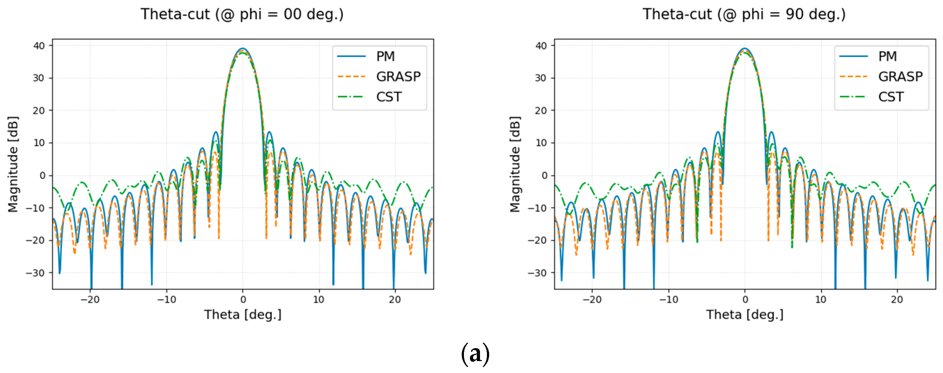
In this paper, the presented method was compared with the results of a radiation characteristic analysis using GRASP by TICRA to analyze the errors associated with the division intervals. The configuration of the parabolic reflector antenna for analysis is given in

Table 1. Configuration of parabolic reflector for analysis.

Parameters	Value
D	$30\lambda$
FD ratio	0.35
$q$ (cosine-q model)	1
Feeder position	(0$\lambda$, 0$\lambda$, 0$\lambda$)
Feeder beam steering angle $\left(\theta , \varphi \right)$	($180°$, $0°$)

.

The division intervals $\left(g_{\psi }, g_{\varphi }\right)$ for comparative analysis varied from 0.1$\lambda$ to 2.0$\lambda$.

Based on the parabolic reflector antenna configuration given in Table 1, Figure 7 depicts the distribution of charge point sources and the radiation characteristic comparison result (theta-cut at $\varphi =0°$) for division intervals $\left(g_{\psi }, g_{\varphi }\right)$ of 0.25$\lambda$, 0.75$\lambda$, 1.25$\lambda$, and 1.75$\lambda$, respectively.

This paper established criteria based on errors in directivity, a 10° reference pattern, and a 45° reference pattern to facilitate a comparative analysis between the results obtained using the presented method and GRASP. The calculation formulas for each criterion are provided in Equations (18)–(20).

$$D_d=\left|F_m-G_m\right|$$

(18)

$$P{E}_{10}=mean\left({\left|F\left(\theta \right)-G\left(\theta \right)\right|}^2\right), \left(-10° \le \theta \le 10°\right)$$

(19)

$$P{E}_{45}=mean\left({\left|F\left(\theta \right)-G\left(\theta \right)\right|}^2\right), \left(-45° \le \theta \le 45°\right)$$

(20)

where $F_m$ and $G_m$ denote the maximum directivity corresponding to the results of each radiation pattern analysis. Additionally, $\theta$ is the observation angle, and $F\left(\theta \right)$ and $G\left(\theta \right)$ represent the radiation patterns (theta-cut at $\varphi =0°$) analyzed using the presented method and GRASP, respectively.

The overall error ($E_T$) is defined in Equation (21) based on the criteria established by Equations (18)–(20). The overall error is a weighted sum based on the importance of each criterion.

$$E_T=10\times D_d+3\times P{E}_{10}+1\times P{E}_{45}$$

(21)

Figure 8 shows the errors for each criterion based on Equations (18)–(20) and the overall error defined by Equation (21) for division intervals $\left(g_{\psi }, g_{\varphi }\right)$ ranging from 0.1$\lambda$ to 2.0$\lambda$, where $g_{\psi }$ and $g_{\varphi }$ are set to the same value.

As is evident from the results in Figure 8, the division intervals $\left(g_{\psi }, g_{\varphi }\right)$ increase sharply at values greater than 0.75$\lambda$. This issue arises from the process of discretizing the continuous effects of the reflector surface for analysis, which can be considered a form of sampling error. As a result of the analysis based on the analysis results of the presented method and GRASP for various division intervals, it is observed that in the technique presented in this paper, when $\left(g_{\psi }, g_{\varphi }\right)$ is equal to or less than ($0.5\lambda , 0.5\lambda$), the results of the two radiation pattern analyses are similar. Therefore, in the method presented in this paper, the surface division intervals $\left(g_{\psi }, g_{\varphi }\right)$ for analyzing the radiation characteristics of a defocus-fed parabolic reflector antenna were set to 0.5λ.

4. Simulation

In this section, the radiation characteristics of various defocus-fed parabolic antenna configurations are analyzed using the presented method, GRASP, and CST. The results are then compared to validate the performance of the method presented in this paper.

4.1. Antenna Configuration

A total of ten parabolic reflectors antennas were configured for comparative analysis, and the detailed configurations are shown in

Table 2. Configuration of parabolic antennas for simulation.

	Parabolic		Feeder
	Diameter [$\mathit{\lambda }$]	FD Ratio	$\mathit{q}$-Factor	Position (x, y, z) [$\mathit{\lambda }$]	Beam Steering ($\mathit{\theta }$, $\mathit{\varphi }$) [$°$]
Case #1	30	0.35	1	(0, 0, 0)	(180, 0)
Case #2	60	0.35	1	(0, 0, 0)	(180, 0)
Case #3	30	0.35	4.5	(0, 0, 0)	(180, 0)
Case #4	40	0.5	2.2	(0, 0, 0)	(180, 0)
Case #5	30	0.35	1	(1, 0, 0)	(180, 0)
Case #6	30	0.35	1	(0, 1.5, 0)	(180, 0)
Case #7	40	0.5	2.2	(0, 0, 2)	(180, 0)
Case #8	40	0.5	2.2	(0, 0, −1)	(180, 0)
Case #9	30	0.35	1	(0, 0, 0)	(160, 0)
Case #10	30	0.35	4.5	(−1, 0, 0)	(160, 0)

.

Figure 9 shows the structure of the parabolic reflector antennas corresponding to each antenna configuration set in Table 1. Additionally, it presents a partial enlargement based on the feeder configuration (position and beam steering direction) and the normalized patterns based on the feeder analysis model (cosine-q model). Note that according to the cosine-q model with q values of 1, 2.2, and 4.5, the directivities are 7.7 dBi, 10.3 dBi, and 13.0 dBi, and the half-power beam widths (HPBWs) are 89.8°, 62.5°, and 44.3°, respectively. Furthermore, the 10 dB beamwidths are 143.1°, 107.3°, and 78.5°, respectively.

4.2. Simulation Analysis Results

Figure 10 compares the radiation characteristics (theta-cut patterns at $\varphi =0°$ and $\varphi =90°$) analyzed using the presented method, GRASP, and CST for each antenna configuration shown in Table 2. In the legend of Figure 10, “PM” represents the presented method.

Table 3. Quantitative comparison of simulation results.

	$\mathit{\theta }$-Cut	Directivity Difference		HPBW Difference		Pattern Difference
	$\mathit{\varphi }$	with GRASP	with CST	with GRASP	with CST	with GRASP	with CST	Region
Case #1	$00°$	0.71 dB	1.38 dB	0$°$	0$°$	0.89 dB	1.05 dB	$-2.7°\le \theta \le 2.7°$
Case #2	$00°$	1.32 dB	0.64 dB	0$°$	0$°$	1.98 dB	1.08 dB	$-1.3°\le \theta \le 1.3°$
Case #3	$00°$	1.13 dB	0.01 dB	0.4$°$	0.1$°$	1.45 dB	0.93 dB	$-5.3°\le \theta \le 5.3°$
Case #4	$00°$	0.65 dB	0.94 dB	0$°$	0$°$	0.59 dB	0.77 dB	$-2.0°\le \theta \le 2.0°$
Case #5	$00°$	0.69 dB	1.35 dB	0.1$°$	0$°$	1.08 dB	0.97 dB	$-10.1°\le \theta \le -1.8°$
Case #6	$90°$	0.65 dB	1.31 dB	0.1$°$	0.1$°$	1.11 dB	1.66 dB	$-12.8°\le \theta \le -4°$
Case #7	$00°$	0.62 dB	0.97 dB	0$°$	0$°$	0.65 dB	0.85 dB	$-6.1°\le \theta \le 6.1°$
Case #8	$00°$	0.41 dB	0.41 dB	0$°$	0$°$	0.74 dB	1.07 dB	$-4.6°\le \theta \le 4.6°$
Case #9	$00°$	0.71 dB	1.16 dB	0$°$	0$°$	0.72 dB	1.28 dB	$-2.8°\le \theta \le 2.8°$
Case #10	$00°$	0.8 dB	0.19 dB	0.4$°$	0.5$°$	0.78 dB	1.74 dB	$-2.3°\le \theta \le 11.4°$

presents the quantitative comparison results for the pattern comparison depicted in Figure 10. This comparison highlights the Absolute Error (AE) differences in gain, the HPBW, and the Mean Absolute Error (MAE) differences of pattern differences within the region of primary interest (near the main beam) for each analysis technique (the presented method, GRASP, and CST). Based on the quantitative comparison results for the various defocus-fed parabolic reflectors listed in Table 2, the presented method, in comparison with GRASP and CST, demonstrated average directivity differences of 0.76 dB (compared with GRASP) and 0.83 dB (compared with CST), average HPBW differences of 0.1 deg. (compared with GRASP) and 0.07 deg. (compared with CST), and average power pattern differences (MAEs) in the region of primary interest of 0.99 dB (compared with GRASP) and 1.14 dB (compared with CST). As is evident from the analysis results in Figure 10, the presented defocus-fed parabolic antenna analysis method in this paper produces results of a very similar shape to those obtained from GRASP and CST. Through these results, it can be confirmed that the presented method can be used to analyze the radiation characteristics of various defocus-fed parabolic reflector antennas.

5. Conclusions

With increasing interest in the W-band, there is a growing focus on parabolic reflector antennas, which are known for efficiently inducing high-gain radiation characteristics. Furthermore, parabolic antennas with defocus-fed configurations have diverse applications, including monopulse tracking, multi-beam formation using multiple feeds, and shared-aperture antennas for multi-band operation. This paper presents a simple method for analyzing the radiation characteristics of defocus-fed parabolic antennas. The derivation of the presented method involves discretely dividing the parabolic surface, accounting for the feeder’s influence at each division point, and employing an electric field analysis using array theory. Additionally, to simplify the method, only scalar functions, not vector fields, were considered. Through applying the presented method to ensure the performance of the radiation characteristic analysis of defocus-fed parabolic reflector antennas, it was confirmed that the maximum division intervals criterion $\left(g_{\psi }, g_{\varphi }\right)$ is 0.5$\lambda ,$ according to the parabolic reflector surface division procedure. To validate the analysis performance of the presented method, which applies this maximum criterion for the division intervals, a comparison was conducted with the analysis results from GRASP and CST. These are representative analysis tools for various defocus-fed parabolic antenna configurations. It was observed that there were differences of only 0.99 dB (compared with GRASP) and 1.14 dB (compared with CST) within the region of primary interest (near the main beam). Consequently, it was confirmed that the presented method in this paper can efficiently analyze the radiation characteristics of various defocus-fed parabolic reflector antennas. The presented method can thus be applied in various areas, such as communication link analysis, beam squint analysis for monopulse tracking, and beam steering region analysis for shared or multi-fed apertures.